Effect of higher-order nonlinearities on amplification and squeezing in Josephson parametric amplifiers
Abstract
Single-mode Josephson junction-based parametric amplifiers are often modeled as perfect amplifiers and squeezers. We show that, in practice, the gain, quantum efficiency, and output field squeezing of these devices are limited by usually neglected higher-order corrections to the idealized model. To arrive at this result, we derive the leading corrections to the lumped-element Josephson parametric amplifier of three common pumping schemes: monochromatic current pump, bichromatic current pump, and monochromatic flux pump. We show that the leading correction for the last two schemes is a single Kerr-type quartic term, while the first scheme contains additional cubic terms. In all cases, we find that the corrections are detrimental to squeezing. In addition, we show that the Kerr correction leads to a strongly phase-dependent reduction of the quantum efficiency of a phase-sensitive measurement. Finally, we quantify the departure from ideal Gaussian character of the filtered output field from numerical calculation of third and fourth order cumulants. Our results show that, while a Gaussian output field is expected for an ideal Josephson parametric amplifier, higher-order corrections lead to non-Gaussian effects which increase with both gain and nonlinearity strength. This theoretical study is complemented by experimental characterization of the output field of a flux-driven Josephson parametric amplifier. In addition to a measurement of the squeezing level of the filtered output field, the Husimi -function of the output field is imaged by the use of a deconvolution technique and compared to numerical results. This work establishes nonlinear corrections to the standard degenerate parametric amplifier model as an important contribution to Josephson parametric amplifier’s squeezing and noise performance.
I Introduction
Driven by the need for fast, high-fidelity single-shot readout of superconducting qubits, superconducting low-noise microwave amplifiers are the subject of intense research. Following the path of Yurke’s et al. work in the late 1980s Yurke et al. (1988, 1989a, 1989b), several designs of Josephson junction-based parametric amplifiers (JPAs) have been introduced Castellanos-Beltran and Lehnert (2007); Yamamoto et al. (2008); Bergeal et al. (2010); Hatridge et al. (2011); Mutus et al. (2013); Eichler and Wallraff (2014); Mutus et al. (2014); Eichler et al. (2014). In addition to high-fidelity superconducting qubit readout leading to the observation of quantum jumps Jeffrey et al. (2014); Vijay et al. (2011), this new generation of near quantum-limited amplifiers have opened up new experimental possibilities such as the creation and tomography of squeezed microwave light Castellanos-Beltran et al. (2008); Mallet et al. (2011); Fedorov et al. (2016), and detailed weak measurement experiments Murch et al. (2013a); Weber et al. (2014); Campagne-Ibarcq et al. (2014). JPAs are now ubiquitous in current superconducting circuit experiments, and applications in other research communities are growing Stehlik et al. (2015); Virally et al. (2016); Simoneau et al. (2017); Goetz et al. (2017).
Depending on their design and operating mode, JPAs can fall in either of two broad categories of linear amplifiers: phase-preserving and phase-sensitive Caves (1982); Roy and Devoret (2016). JPAs in the former category amplify both quadratures of the signal and quantum mechanics put a strict lower bound on the noise added by this process. On the contrary, JPAs in the latter category can amplify the signal of a single quadrature without any added noise by proportionally attenuating the conjugate quadrature. In other words, a phase-sensitive amplification is a source of squeezed radiation Walls and Milburn (2008); Gardiner and Zoller (2004). The properties of JPAs as a source of squeezed light are therefore intimately related to their noise properties as a phase-sensitive amplifier. While JPAs are usually modeled as quantum-limited amplifiers, and thus perfect squeezers, experimental results indicate that nonidealities limits both the achievable level of squeezing Zhong et al. (2013); Murch et al. (2013b); Bienfait et al. (2016) and the measurement quantum efficiency Murch et al. (2013a, b); Vijay et al. (2012); Weber (2014).
We show that these nonidealities are linked to higher-order corrections to the JPA Hamiltonian due to the Josephson cosine potential. We go beyond the standard analytical results by considering numerical solutions to the quantum master equation, including these usually neglected higher-order corrections. We derive the corrections to the JPA Hamiltonian for the single-mode and single-port lumped-element JPA Roy and Devoret (2016); Hatridge et al. (2011). Using the formalism of quantum optics, we compare three frequently used pumping schemes of the JPA: monochromatic current pump Hatridge et al. (2011); Yurke and Buks (2006), bichromatic current pump Kamal et al. (2009), and monochromatic flux pump Yamamoto et al. (2008); Wustmann and Shumeiko (2013); Zhou et al. (2014). We derive the leading higher-order corrections for each and study numerically their effect on gain, quantum efficiency, squeezing level and gaussianity of the output field. In addition, by comparing numerical results to an experimental characterization of the JPA output field, we show that the squeezing level saturation previously reported in the literature Murch et al. (2013b); Zhong et al. (2013) can be explained by including leading non-quadratic corrections in the Hamiltonian. The focus of this work on higher-order corrections complements recent theoretical investigations of various JPA designs Yurke and Buks (2006); Kamal et al. (2009); Wustmann and Shumeiko (2013); Eichler (2013); Kochetov and Fedorov (2015); Roy and Devoret (2016).
The paper is organized as follows. In Sec. II, we set the notations and recall useful results for the standard quantum optics model of the degenerate parametric amplifier (DPA). In Sec. III, we introduce the lumped-element JPA and the three different pumping schemes investigated in this work. For each scheme, we derive the higher-order corrections and show how, in the low gain and low nonlinearity regime, the system can be mapped back to the DPA. The respective advantages of the three pumping schemes are compared. In Sec. IV, we compare the intracavity field properties of the different schemes including deviations from the results of the DPA. We also show that higher-order corrections can lead to non-Gaussian intracavity fields. In Sec. V, we characterize the JPA as an amplifier by calculating the gain and the quantum efficiency for both the phase-sensitive and phase-preserving modes of operation. In order to relate these results to a series of experiments Zhong et al. (2013); Murch et al. (2013b); Bienfait et al. (2016), in Sec. VI we focus on the phase-sensitive amplification of vacuum, i.e. squeezed vacuum. We characterize the JPA as a source of squeezed light by calculating moments and cumulants of the filtered output field. This allows us to obtain the squeezing level of the light generated, as well as to estimate its non-Gaussian character. In this section, numerical results are discussed together with an experimental characterization of the output field, including a direct imaging of the non-Gaussian distortions of the field due to nonidealities. Finally, Sec. VII summarizes our work.
II Degenerate parametric amplifier in a nutshell
To set the notation, we begin by presenting the DPA model and its solution Gardiner and Zoller (2004); Yurke and Buks (2006); Laflamme and Clerk (2011). In the next sections, we show how the JPA can be mapped to the DPA and study deviations from this simple model due to higher-order corrections.
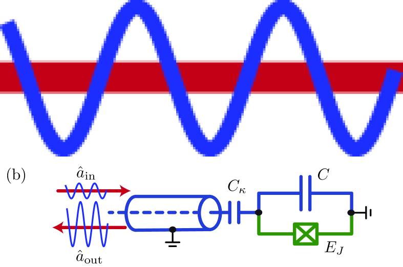
The DPA is a standard model of quantum optics exhibiting parametric amplification and squeezing. In this model, as illustrated in Fig. 1(a), a nonlinear medium inserted in a single-mode cavity is pumped in order to modulate its refractive index at twice the cavity frequency Walls and Milburn (2008). This modulates the effective length of the cavity and, as a consequence, its frequency. This modulation acts as an external source of energy leading to parametric amplification Landau and Lifshitz (1969); Nation et al. (2012).
Introducing the annihilation (creation) operator for excitations in the cavity, the DPA Hamiltonian is (setting for the remainder of the paper)
| (1) |
with the cavity frequency, the nonlinearity, and , the annihilation (creation) operator of an excitation in the external pump mode. In the strong classical pump regime where and in a frame rotating at half the parametric pump frequency , the Hamiltonian is Collett and Gardiner (1984); Walls and Milburn (2008)
| (2) |
with the detuning and the amplitude of the parametric pump.
Using input-output theory Gardiner and Zoller (2004); Walls and Milburn (2008), the equation of motion for the intracavity field is
| (3) |
where the input mode (coupled to the cavity with rate ) carries the signal to be amplified, while the input mode (coupled to the cavity with rate ) mixes additional vacuum noise to the signal due to undesired losses. The total damping rate of the cavity is given by .
As shown in Appendix A, the solution to Eq. (3) can be obtained in Fourier space. Using the boundary condition Gardiner and Zoller (2004); Walls and Milburn (2008)
| (4) |
where is the output field carrying the amplified signal, one obtains the solution
| (5) |
where the signal and idler amplitude gains are defined as
| (6) | ||||
| (7) |
with , and the frequency defined in the rotating frame such that a signal at is in resonance with the rotating frame frequency . The output signal at frequency mixes and amplifies the input signal and idler modes at frequencies . In the lossless case (), the signal and idler gains obey and the input-output relation is a unitary squeezing transformation Caves (1982). On the contrary, in the presence of losses (), additional noise is mixed with the input signal and the DPA is not a quantum-limited amplifier.
If the measurement bandwidth includes both the signal and idler modes, these two modes act effectively as a single mode and the DPA is a phase-sensitive amplifier. On the contrary, if the idler frequency () falls outside the measured frequency band, the idler mode acts as a noise mode and the DPA is a phase-preserving amplifier with phase-preserving photon number gain Caves (1982); Eichler (2013)
| (8) |
Hence, depending on the experimental details, the same system can act either as a phase-sensitive or phase-preserving amplifier. The same will hold true for the JPA, and we will thus consider both cases when characterizing the JPA properties as an amplifier in Sec. V.
Finally, in both operating regimes, the gain diverges () at the parametric threshold Laflamme and Clerk (2011); Wustmann and Shumeiko (2013)
| (9) |
and large gain is obtained near but below this value. Indeed, above the threshold spontaneous parametric oscillation effects will occur leading to the generation of photons activated by vacuum and thermal fluctuations Wilson et al. (2010); Wustmann and Shumeiko (2013). In this work, we focus on parameter regimes where the DPA act as an amplifier and thus is always considered.
III Higher-order corrections to the JPA: Comparison of pumping schemes
In this section, we introduce the standard lumped-element JPA circuit and consider three pumping schemes: the monochromatic current pump, the bichromatic current pump and the monochromatic flux pump. We show how these amplifiers can be mapped back to the DPA model, and compare their respective advantages. Importantly, for each pumping scheme, we derive the leading nonidealities which cause deviations from the DPA model. The study of these deviations in the following sections constitutes the core of our results.
III.1 JPA circuit
As illustrated in Fig. 1(b), the lumped-element JPA is simply a capacitively shunted Josephson junction coupled to a transmission line Yurke et al. (1988); Hatridge et al. (2011). The Hamiltonian of this standard circuit is
| (10) |
with the capacitance, the Josephson energy, the reduced flux quantum, the charge and the generalized flux. As usual, the charge and the flux are conjugate quantum operators obeying .
Expanding the cosine and introducing bosonic annihilation (creation) operator , one obtains Bourassa et al. (2012)
| (11) |
with the bare frequency of the resonator, the charging energy and the unitless zero point flux fluctuations.
As JPAs are usually weakly nonlinear devices, the next step is to perform a quartic potential approximation by keeping only the first correction to the standard harmonic oscillator
| (12) |
with the Kerr coefficient . As the leading neglected correction is of order , this approximation is valid in the regime which is relevant for typical JPA frequencies and Kerr nonlinearities corresponding to to Bourassa et al. (2012). We note that the Transmon qubit has the same circuit and Hamiltonian as a JPA but operates at larger Kerr nonlinearities Koch et al. (2007).
In the rotating-wave approximation (RWA), also valid for , we obtain the standard Kerr Hamiltonian
| (13) |
with the renormalized oscillator frequency. By normal ordering and performing the RWA prior to the quartic potential approximation, corrections from all orders renormalizes the resonator frequency and the Kerr nonlinearity Leib et al. (2012). To keep the notation light, we neglect this simple renormalization of parameters in the present work.
While the Kerr Hamiltonian was obtained from the lumped-element circuit, the same Hamiltonian with renormalized parameters would apply for a distributed nonlinear resonator in the single-mode approximation Bourassa et al. (2012); Eichler and Wallraff (2014), or a lumped-element JPA with additional linear inductances Zhou et al. (2014). However, it is worth noting that, in both cases, the additional inductances can reduce the validity of the quartic potential approximation. See Ref. Eichler and Wallraff (2014) for details.
As discussed in Sec. II, in order for this system to act as a parametric amplifier a pump must modulate one of the parameters at twice the resonance frequency. We now consider three pumping schemes leading to such a modulation.
III.2 Monochromatic current pump
We first consider the standard current-pumped JPA Yurke et al. (1988, 1989a, 1989b); Castellanos-Beltran and Lehnert (2007); Hatridge et al. (2011); Yurke and Buks (2006); Eichler and Wallraff (2014). In this scheme, a single current pump near resonance with the oscillator is used. Due to the Josephson relations, the junction acts as a current-dependent nonlinear inductance with Manucharyan et al. (2007)
| (14) |
For a monochromatic current pump , the first nonlinear contribution to the inductance is the cosine squared, which leads to a modulation of the inductance at twice the pump frequency.
Using standard circuit quantization techniques Devoret (1995) and using the quantum optics language, the current pump is equivalent to adding a single-photon drive, such that the total Hamiltonian of the pumped circuit is
| (15) |
where and are the pump amplitude and frequency. In a frame rotating at the pump frequency, it is useful to eliminate the pump Hamiltonian using a displacement transformation, which leads to , with the classical field and the quantum fluctuations Yurke and Buks (2006); Laflamme and Clerk (2011), see Appendix B for details. In this displaced frame, the Hamiltonian takes the form
| (16) |
with the shifted detuning due to the cavity population
| (17) |
the effective parametric pump strength , and the classical field obeying the nonlinear differential equation
| (18) |
In general, the steady state of this cubic equation can exhibit bifurcation physics Yurke and Buks (2006); Manucharyan et al. (2007). However, for the current-pumped JPA, the bifurcation threshold coincides with the parametric threshold and in the context of parametric amplification, parameters are chosen to be below the bifurcation point Laflamme and Clerk (2011). Thus, in what follows, is always a single-valued function.
For simplicity, in Eq. (16) was obtained by performing the quartic approximation before the displacement transformation. However, one can perform the displacement transformation on the full cosine potential, before performing the RWA and the quartic potential approximation. These corrections, which mainly shift the operating frequency and bifurcation point of the amplifier have been studied in details in Ref. Kochetov and Fedorov (2015).
The displaced Hamiltonian of Eq. (16) also includes the nonlinear corrections to the single pump scheme
| (19) |
with the cubic term coefficient and the standard quartic Kerr coefficient . These corrections originate from the displacement of the Kerr nonlinearity. In order to obtain linearized equations, they can be neglected in the small quantum fluctuations limit Yurke and Buks (2006). In the following sections, we will explore the validity of this approximation and show that it is valid in the low gain and low Kerr nonlinearity regime.
When neglecting the corrections , the displaced Hamiltonian can be related to with the mapping , , , and . Thus, in this linear regime, the monochromatic current-pumped JPA is equivalent to the DPA, but in a displaced frame. From the lab frame, this implies that while the output of a DPA is squeezed vacuum, the output of this current-pumped JPA is a displaced squeezed state.
III.3 Bichromatic current pump
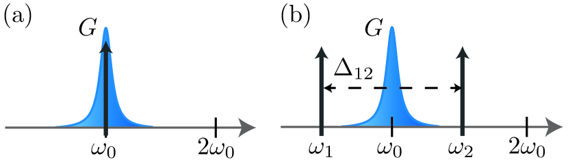
We now consider an alternative scheme with two current pumps of frequencies and that are chosen such that Kamal et al. (2009). As shown in Fig. 2, while in the monochromatic case the pump is at a frequency close to the amplified signal [panel (a)], in the bichromatic case the pumps are separated spectrally from the signal [panel (b)].
Similar to Eq. (15), the starting Hamiltonian is
| (20) |
with and the frequencies and amplitudes of the two pumps. In order to remove the pumps in a similar way as in the monochromatic case, we consider two displacement transformations instead of one. This allows to consider two classical fields, each rotating at one of the pump frequencies, and to separate them from the quantum fluctuations of the cavity mode possibly rotating at a third frequency.
Choosing a frame rotating at the average pump frequency , the double displacement transformation leads to
| (21) |
A more detailed and formal treatment of the transformation is presented in Appendix B. By applying this transformation, one obtains
| (22) | ||||
with the shifted detuning
| (23) |
and the effective parametric pump strength . All the rotating terms are grouped in the Hamiltonian
| (24) | ||||
where is the detuning between the two pump frequencies. Finally, we define
| (25) |
the nonlinear correction to the Hamiltonian.
The rotating Hamiltonian can be dropped by a RWA. Assuming symmetric pumps (), this RWA is valid for . Since the effective parametric pump strength is bounded by the parametric threshold defined in Eq. (9), one can choose the detuning in order to enforce the validity of the RWA. For zero detuning in Eq. (22) (), the RWA condition is simply . An advantage of the bichromatic pump compared to the monochromatic pump is thus that the cubic terms () are now rotating and can be safely neglected. This reduces the nonidealities of the amplifier, and implies that, with respect to the monochromatic current pump, the bichromatic current-pumped JPA acts as an ideal phase-sensitive amplifier for a larger parameter range (see Sec. IV).
Again, in the small quantum fluctuations limit, we can neglect the higher-order correction . Under this approximation, the system is related to the DPA with the mapping , , and
| (26) |
Whereas in the monochromatic case the pump leads to a displacement of the output field at the center frequency of the amplified band, in this case the two pumps lead to displacements far detuned from the band of interest. This spectral separation allows to filter the pumps without the need for a more involved pump cancellation scheme Eichler (2013).
| Pumping scheme | Monochromatic current | Bichromatic current | Monochromatic flux |
| Spectral separation | No | Yes | Yes |
| Spatial separation | No | No | Yes |
| Output state 111 We use the standard notation of quantum optics where and are respectively the displacement and squeezing operators Barnett and Radmore (1997). | |||
| Effective parametric pump () | |||
| Pump induced frequency shift () | |||
| Relative shift () 222 We introduce the compact notation , and . | |||
| Corrections () |
III.4 Monochromatic flux pump
Current pumps are an indirect way to modulate the inductance of the JPA by using the nonlinearity of the Josephson junction. A well-studied alternative is to use an adjustable inductance that can be directly modulated. In superconducting circuits, this can be done by replacing a single Josephson junction by a SQUID, a flux-dependent nonlinear inductance. With this slight modification of the circuit, parametric amplification can be obtained by flux-pumping. This pumping scheme has been extensively studied both experimentally Yamamoto et al. (2008); Zhou et al. (2014); Krantz et al. (2013) and theoretically Wustmann and Shumeiko (2013). Here, we derive the Hamiltonian of the flux-pumped JPA similarly to Ref. Wustmann and Shumeiko (2013), with an additional focus on higher-order corrections to the Hamiltonian.
Replacing the Josephson junction by a SQUID modifies the Josephson energy in the equations of Sec. III.1 such that Tinkham (2004)
| (27) |
where is the external flux applied in the SQUID loop. In order to obtain parametric amplification, the external flux is modulated at frequency , with an additional static component chosen such that Wustmann and Shumeiko (2013)
| (28) |
with the unitless static flux and the modulation amplitude.
In order to separate the harmonics of the pump, we Fourier expand the flux-dependent Josephson energy
| (29) |
where the coefficients of the expansion are given in Appendix C. In the relevant limit of small pump amplitude (), one obtains that the leading contribution of each Fourier coefficient is and the expansion of Eq. (29) can be safely truncated.
Due to the flux modulation, the result of the RWA on Eq. (12) is modified and the Hamiltonian is
| (30) |
with the detuning and the effective parametric pump strength . In the quartic potential approximation, the non-quadratic corrections to the Hamiltonian are now
| (31) |
with the Kerr nonlinearity renormalized by the flux modulation.
While the Kerr nonlinearity is essential for parametric amplification in the current-pumped cases, the parametric pump strength of the flux-pumped JPA is independent of this quantity. It is merely an artifact of the use of Josephson junctions to build a flux-dependent inductance. More explicitly, in the limits of a resonant pump and a small pump amplitude , the ratio of the parametric pump strength to the parametric threshold is
| (32) |
with the JPA quality factor Zhou et al. (2014). This ratio is independent of the Josephson energy or of the Kerr nonlinearity.
For standard JPA quality factors 10-100, and static flux bias such that , Eq. (32) implies that parametric pump strengths close to the parametric threshold can be obtained even in the small flux-pump limit . Thus, the leading correction to the JPA Hamiltonian is the first term of Eq. (31) which is independent of . The other corrections, respectively linear and quadratic in , can be dropped in this small flux modulation limit. This implies that the leading higher-order correction to the flux-pumped JPA is the same as in the bichromatic current pump case () and thus the flux-pumped JPA Hamiltonian reads
| (33) |
Again, in the limit of small quantum fluctuations, higher-order corrections can be dropped and the JPA related to the DPA model with the mapping and . Since there is no displacement transformation, this pumping scheme is more closely related to the DPA than the current-pumped JPAs.
III.5 Summary and comparison of pumping schemes
Table 1 compares and summarizes the pumping schemes reviewed in this section. It is divided in two parts: the first presents general properties of each pumping scheme, while the second summarizes expressions for parameters, and leading higher-order corrections to the ideal DPA Hamiltonian.
The first distinction to make between these schemes is the spatial and spectral separation of the pump and signal. In the flux pump case, two distinct ports are used for the signal and the pump, while in the current pump cases the same input port is used for both the pump and the signal. Hence, while the output of the flux-pumped JPA is squeezed vacuum, the output of the current-pumped JPAs is displaced due to reflected pump field(s). In the bichromatic case these fields are far detuned from the amplified signal and can be filtered out prior to the measurement. On the contrary, in the monochromatic case the reflected pump is at the frequency where the amplifier gain is maximal. This implies that great care must be taken to either cancel the pump or separate it from the signal Eichler (2013).
Moreover, all three pumping schemes lead to a negative pump-induced frequency shift of the resonator. While in the case of the current pumps, the shift follows from the population of the nonlinear cavity by the pump field(s), in the case of the flux pump, the shift is a geometric effect due to the cosinusoidal dependence of the SQUID’s Josephson energy on the external magnetic flux Wustmann and Shumeiko (2013); Krantz et al. (2013). These pump-induced detunings obey the relation
| (34) |
where the superscript is used to note that we are considering the pump-induced shift. Note that for the current pumps this shift scales as , while in the flux pump case it scales as (see Table 1).
Finally, we note that while the leading higher-order correction is the same for the bichromatic current pump and the flux pump, the monochromatic current pump Hamiltonian has additional cubic corrections. This implies that, without any change to the actual amplifier circuit (fixed parameters), using a bichromatic current pump instead of a monochromatic current pump decreases the nonidealities of the JPA.
IV Signature of higher-order corrections in the intracavity field
In order to evaluate the impact of the higher-order corrections discussed in the previous section, we numerically compute first and second order moments of the steady-state intracavity field. These quantities show that, while the JPA acts as an ideal DPA in the low nonlinearity regime, the higher-order corrections can play a significant role in the presence of larger nonlinearities. To give a more intuitive representation of the effect of the nonidealities on the amplifier state, we also calculate Wigner functions of the intracavity field.
The numerical results of this section are obtained by finding the steady-state solution of the master equation
| (35) |
where , are the higher-order corrections considered, and is the standard dissipation superoperator Gardiner and Zoller (2004); Walls and Milburn (2008).

IV.1 Deviation from standard DPA results
With the ideal DPA model, the first order moment of the intracavity field is . However, in the case of the monochromatic current-pumped JPA, the cubic corrections act as an effective pump leading to an additional displacement of the field and thus a nonzero first moment. To understand this effect, one can consider a mean-field treatment of the cubic corrections, where Eichler and Wallraff (2014)
| (36) |
with , and the second-order moments of the JPA state. Under this approximation, the cubic terms act as an additional state-dependent pump and can be eliminated by a second displacement transformation. Such a mean-field treatment was used to study pump depletion effects and the dynamic range of the JPA in Ref. Eichler and Wallraff (2014).
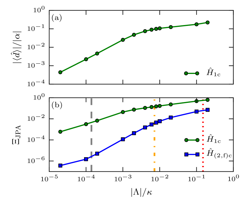
A mean-field solution would require the self-consistent solution for , . Instead, we numerically find the steady-state of the master equation Eq. (35). Fig. 3(a) shows the ratio of the displacement induced by the cubic terms, to the steady-state solution of Eq. (18) for the displacement field . While negligible in the low nonlinearity limit, the induced displacement becomes significant for larger Kerr nonlinearities. On the contrary and as expected from mean-field, no additional displacement is observed for the the bichromatic current and monochromatic flux pumps cases.
We now consider signatures of the corrections in the second order centered moments , and , where the subscript DPA, JPA refers to the model that is used. It follows from Heisenberg uncertainty principle that, for any state, these moments obey the relation
| (37) |
where the equality is only obtained for pure states Gardiner and Zoller (2004). From the analytical solution to the DPA model (see Sec. II and App. A), one obtains a value of below this bound
| (38) |
This result can be understood from the fact that, due to damping, the steady-state of the DPA is not a pure squeezed state Collett and Gardiner (1984).
To quantify the deviation of the JPA moments from the expected results of an ideal DPA due to the corrections, we define the deviation
| (39) |
where , are the centered moments of the JPA intracavity field, here calculated numerically including higher-order corrections. The deviation is zero in the case of an amplifier that maps exactly to a DPA (negligible higher-order corrections) and increases towards one as the corrections to the DPA Hamiltonian become important.
As observed in Fig. 3(b), the deviations increase with the amplitude of the Kerr nonlinearity. The additional cubic terms of lead to larger deviation for the same parameters. Thus, by simply using two current pumps instead of one, the deviation from the expected results for a DPA are reduced by approximately two orders of magnitude. To put in context the range of Kerr nonlinearity considered, the vertical lines indicate approximate experimental parameters of three recent experiments with JPAs Eichler (2013); Hatridge et al. (2011); Murch et al. (2013b). We note that, in practice, the smaller nonlinearity (dashed gray line) is obtained using junction arrays. Indeed, the Kerr nonlinearity with a junction array is inversely proportional to the square of the number of junctions in the array Castellanos-Beltran and Lehnert (2007); Eichler and Wallraff (2014).
IV.2 Phase space representation
In order to visually represent the deviation from the DPA, we present in Fig. 4 the Wigner function of the intracavity field for increasing Kerr nonlinearities (from left to right). For each value of , we present results for the monochromatic current-pumped JPA (including cubic and quartic corrections ) in the top panels and for the bichromatic current-pumped (quartic correction ) or equivalently the flux-pumped JPA in the bottom panels. In all cases, we consider a phase-preserving gain of dB. While in the low nonlinearity case presented in panels (a) we observe a quadrature squeezed state for both type of corrections, in the increased nonlinearity of panels (b) non-Gaussian signatures appear in the monochromatic pump case. Increasing even more the nonlinearity amplitude in panels (c,d), both types of corrections lead to non-Gaussian signatures.
In the limit of large nonlinearity , we observe that the shape of the Wigner function varies with the pumping scheme. In the monochromatic current pump case, we observe the so-called crescent or banana-shaped deformation of the distribution Dodonov and Man’ko (2003). Similar distributions have been observed in the transient dynamics of a driven Kerr nonlinear resonator. In particular, the large nonlinearity regime as been well studied both theoretically Wilson-Gordon et al. (1991), and experimentally in superconducting circuits Kirchmair et al. (2013).
In the case of a single Kerr-type correction, we observe a more symmetric “S”-shaped Wigner function deformation. In the case of the flux-pumped JPA, “S”-shape features have been predicted theoretically and observed experimentally using a semi-classical analysis of the phase-dependence of the JPA response Wustmann and Shumeiko (2013); Bienfait et al. (2016). This deformation of the Wigner function is also consistent with experimental studies imaging the JPA output field, see Sec. VI.4.
From the observed deformation of the Wigner function in panels (c,d), one can expect the higher-order corrections to limit the squeezing produced by a JPA. Such a saturation of squeezing has been observed experimentally Murch et al. (2013b); Zhong et al. (2013), and will be discussed in more details in Sec.VI.2. In addition, one can expect the output field of the JPA to exhibit significant non-Gaussian signatures for large gain and nonlinearity. Both the squeezing level and the non-Gaussian character of the output field are characterized more quantitatively in Sec. VI. More generally, the results of this section indicate that, for the same parameters, the additional cubic terms in the monochromatic current pump case lead to additional nonidealities limiting JPA performance.
V Gain and quantum efficiency
To characterize the effect of higher-order corrections on amplifier properties, in this section we numerically compute the low power gain and added-noise number of the JPA. From these, we obtain the phase-sensitive and phase-preserving quantum efficiency of the amplifier.
V.1 Phase-sensitive and phase-preserving gain
The gain is computed by considering the linear response of the JPA to a narrow-band signal probe or, in other words, the same approach as is used experimentally. More concretely, starting from the steady-state solution of the JPA master equation Eq. (35), we add to the Hamiltonian the probe field
| (40) |
with the drive amplitude, and find the new steady-state under this weak drive. From the displacement of the cavity field generated by the probe, one can calculate the output field response. As is already made clear from Eq. (5), the gain is a function of the probe frequency. Using a time-independent probe, we compute the JPA gain at the center frequency .
As discussed in Sec. IV, the cubic corrections in the Hamiltonian of the monochromatic current-pumped JPA also induce a displacement of the cavity field. This additional displacement modifies the bifurcation point of the system, something that can lead to instabilities in the numerical calculations. Hence, this section considers only the effect of a Kerr-type correction, which is the leading correction for the bichromatic current pump and the monochromatic flux pump. In the case of the monochromatic current pump, the additional cubic terms could lead to corrections which, following the results of the previous sections, would appear at lower gain and nonlinearity than those due to the quartic term.
To study the linear response regime, we limit our analysis to a low-power probe where . While an analysis of the dependence of the gain on the probe amplitude would allow to calculate the dynamic range of the JPA Eichler and Wallraff (2014); Kochetov and Fedorov (2015), this is beyond the scope of this paper.
Using the input-output relation Eq. (4), the displacement generated by the probe and the input field amplitude , we can compute the gain matrix whose elements are defined by the linear input-output equation
| (41) |
where we have defined the standard quadratures , and . By considering separately the response to two probes with orthogonal phases, we can calculate all elements of the gain matrix.
To obtain the phase-preserving gain, we express the above quadrature input-output relation in terms of field operators. Using Eqs. (5) and (8), we then find that the JPA phase-preserving gain is related to the phase-sensitive gain matrix by
| (42) |

Fig. 5 presents the phase-preserving gain, as well as the elements of the phase-sensitive gain matrix for a JPA with increasing Kerr nonlinearities. These quantities are plotted as a function of the phase-preserving gain calculated from Eq. (8) for an ideal DPA. As expected, Fig 5(a) shows that, in the low nonlinearity regime (blue diamonds), the JPA phase-preserving gain is equal to the ideal DPA gain and the corrections are negligible. As the Kerr nonlinearity increases (green squares and red circles) the JPA nonidealities result in a decreased gain, with deviations increasing with gain.
Fig 5(b) presents the diagonal elements of the phase-sensitive gain matrix, while Fig 5(c) shows the off-diagonal elements. In the low gain regime, as expected for a phase-sensitive amplifier, the diagonal elements are inversely proportional with one quadrature amplified and the other attenuated. In this regime, the gain matrix is diagonal. When the off-diagonal terms become significant, the attenuation coefficient starts to increase, deviating significantly from the expected behavior of an ideal phase-sensitive amplifier.
For higher gain and nonlinearities, the gain matrix is not symmetric and cannot be diagonalized with orthogonal eigenvectors. In this regime, the amplification process mixes quadratures. Noting that a similar effect occurs for a DPA with pump-cavity detuning Laflamme and Clerk (2011), we can interpret the effect of the nonlinearity as a gain-dependent detuning of the system. Hence, for a given gain choosing a slightly different detuning could mitigate higher order effects and reduce quadrature mixing. This implies that when higher-order corrections are important, the optimal phase and frequency of operation of the JPA is gain-dependent. The interplay of the optimal frequency of operation and nonlinear corrections has recently been the subject of experimental investigation in a similar device Liu et al. (2017).
V.2 Phase-preserving quantum efficiency
To characterize the effect of Kerr-type correction on the JPA noise properties, we now evaluate its added-noise and quantum efficiency. As illustrated in Fig. 6, the quantum efficiency can be interpreted as the transparency of a fictitious beam splitter added at the input of a noiseless amplifier in order to model the noise added by the amplification as additional input vacuum noise Leonhardt and Paul (1994); Mallet et al. (2011).

With this picture in mind, we define the quantum efficiency such that the input-output field fluctuations are related by
| (43) |
with the symmetrized fluctuations of an operator
| (44) |
Note that the case corresponds to having no output signal and is therefore not relevant here. The first term of Eq. (43) is the added noise due to the amplification process, represented as vacuum fluctuations in Fig. 6, while the second term is fluctuations in the input signal. It is useful to express Eq. (43) in a simpler form
| (45) |
where is the added noise referred to the input. Using the inequality , one can derive the well-known quantum limit for a phase-preserving amplifier Caves (1982)
| (46) |
which simplifies in the large gain limit to .
Using these definitions, the quantum efficiency can be expressed as
| (47) |
where we have used the quantum limit of Eq. (46). This inequality implies, in the large gain limit, that the bound on the quantum efficiency of a phase-preserving measurement is . This result simply reflects the well-known fact that ideal phase-preserving amplification can be obtained by the use of two ideal phase-sensitive amplifiers and a beam splitter which adds vacuum fluctuations Caves (1982).
Note that the alternative definition of the quantum efficiency is also found in the literature, with a number of added noise photons. This definition relates the amplifier performance to an ideal phase-preserving amplifier instead of a noiseless amplifier. However, this expression implicitly assumes the large gain limit of Eq. (46) and therefore overestimates the quantum efficiency in the low gain regime where cannot be neglected. In this work, we will consider the definition of Eq. (47), as this allows to treat phase-preserving and phase-sensitive amplification on the same footing and is independent of gain.
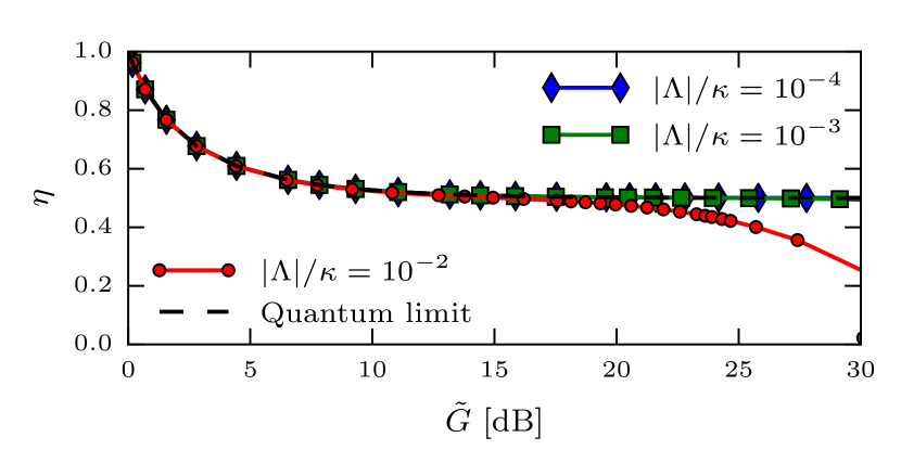
Fig. 7 shows the quantum efficiency in the phase-preserving case as a function of gain and for three Kerr nonlinearities. In the low gain regime, all curves are equal to the quantum limit. For higher gains, the Kerr nonlinearity leads to a decreased quantum efficiency. These results are obtained by numerically calculating the gain and the output field spectrum of the amplifier, with
| (48) |
In this calculation, we neglect any bandwidth or detuning effect and consider the zero frequency component of the spectrum.
Surprisingly, even for a significant phase-preserving gain dB, and Kerr nonlinearity , the JPA with Kerr-type corrections is nearly quantum-limited without any tuning of parameters. On the contrary, we will show in the following section that the same Kerr-type correction strongly influences the quantum efficiency of a phase-dependent measurement. In that case, a careful choice of the phase of operation of the JPA is essential in order to obtain near quantum-limited amplification.
V.3 Phase-sensitive quantum efficiency
We now generalize the concepts of the previous section to the case of phase-sensitive amplification. Contrary to the simpler case of phase-preserving amplification, the quantum efficiency is not a single number, but rather a function of the measurement phase . Hence, one must choose the measured quadrature in order to maximize quantum efficiency.
For the ideal DPA, no noise is added independently of the phase considered and for all . In that specific case, the quantum efficiency of the full measurement chain Pozar (1997) is maximized for the measurement phase which maximizes the gain . However, when including a Kerr correction, we have shown in Sec. V.1 that the gain matrix becomes non-symmetric. In that case, the nonzero leads to quadrature mixing during the amplification, which can be seen as a source of added noise. Thus, we will show that contrary to the ideal DPA, in the presence of a Kerr correction, the maximal quantum efficiency is not obtained by maximizing but rather by minimizing . We note the phase of the quadrature which minimizes the mixing of noise with the signal.
More formally, in order to characterize the field fluctuations, we define the matrix of the symmetrized moments as the matrix analog of Eq. (44) Caves (1982)
| (49) |
with , and the anticommutator. Similarly, the added-noise matrix is defined through a generalization of Eq. (45)
| (50) |
We note that the product of the diagonal elements of this matrix are bounded by the quantum limit to amplification Caves (1982)
| (51) |
For the standard lossless DPA, we obtain noiseless amplification since and .
In the presence of Kerr correction, to make explicit the choice of the measurement phase, we define the phase-dependent added noise
| (52) |
as the first diagonal element of the rotated added-noise matrix, with the counter-clockwise orthogonal rotation matrix. From this, we define the phase-dependent quantum efficiency . While we focus in the following on the diagonal element of the added-noise matrix, with characterizing the noise added to the amplified quadrature, in general is non-diagonal and the amplification can lead to added cross-correlations between the quadratures.
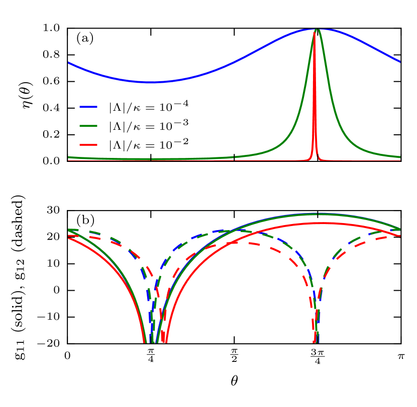
Fig. 8 shows the quantum efficiency and gain as a function of the quadrature phase for increasing values of . In Fig. 8(a), we observe that the quantum efficiency oscillates with and becomes increasingly peaked around a value of the phase with increasing nonlinearity. For a fixed nonlinearity, increasing the gain leads to the same effect (not shown). We note that the position of the peak in the quantum efficiency correlates with a dip in the off-diagonal matrix element shown in Fig 8(b). This dip is shifted to a narrower range of phases as the Kerr nonlinearity is increased. This is in agreement with Fig. 5(c) which showed that, for a fixed quadrature phase, increasing the nonlinearity leads to larger and thus requires a larger phase correction. Thus, as expected the quantum efficiency is maximized when the noise added through quadrature mixing is minimized.
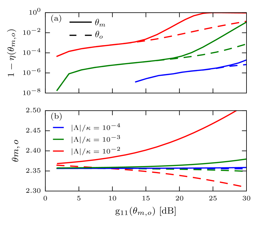
Fig. 9 presents as a function of phase-sensitive gain for increasing Kerr nonlinearities. To further illustrate the importance of choosing the appropriate phase, results for both the optimal phase of minimal cross-gain (dashed curves), and for the non-optimal phase of maximal gain (, solid curves) are shown. As expected, the quantum efficiency is reduced [larger ] for increased gain and nonlinearities. Strikingly, when considering a gain of 25 dB and , the quantum efficiency at phase is around 0.9, while it is closed to zero for . Fig 9(b) shows that this dramatic difference in performance is obtained with less than rad (12 degrees) difference in phase.
These results points to both the Kerr nonlinearity and the non-optimal choice of measurement phase as a possible explanation for a series of experiments that have reported smaller than expected quantum efficiencies for JPAs Murch et al. (2013a, b); Vijay et al. (2012); Weber (2014). A more detailed experimental study of the quantum efficiency as a function of both detuning and measurement phase could confirm these results and would allow for a better understanding of these nonlinear effects.
VI Output field characterization
Following the results of the previous sections, one can expect to also find signatures of the nonidealities in the JPA output field, including in squeezing experiments. In this section, we compute moments of the output field which allow to characterize the JPA as a source of squeezed light. Following the results of Sec. IV and more generally for Kerr cavities Dodonov and Man’ko (2003); Kirchmair et al. (2013), we expect the higher-order corrections to lead to a non-Gaussian output field. To verify this, we calculate third and fourth order cumulants which reveal departure from gaussianity.
Throughout this section, we compare our numerical results to an experimental characterization of the output field of a flux-driven JPA. Moments of the JPA output field are obtained using a single-path reconstruction method Eichler et al. (2011), while a full output field imaging is obtained from a deconvolution technique. Details of the experimental setup and methods are presented in Appendix D.
VI.1 Filtered output field : Definition and numerical technique
In order to compare our numerical results to experimental data, we consider the finite bandwidth of the measurement chain in our calculations. To this end, we define the filtered output field as the convolution of the full output field da Silva et al. (2010):
| (53) |
with a filter function normalized such that , in order to ensure standard bosonic commutation relations . The moments of this field can be evaluated by numerical integration of correlation functions using the quantum regression formula Gardiner and Zoller (2004). The details of the numerical technique are presented in Appendix E. We note that the complexity of the calculation scales exponentially with the order of the moment considered da Silva et al. (2010). As a result, fourth order moments are at the limit of our current computational capacities. Fortunately, this is sufficient to characterize the departure from ideal Gaussian behavior. Unless otherwise specified, the filter used is a time-domain boxcar filter of 256 ns (bandwidth of approximately 4 MHz), which coincides with the experimental method.
VI.2 Squeezing level
In order to characterize the squeezing produced by the JPA, we calculate the filtered output field squeezing level defined as Zhong et al. (2013)
| (54) |
with the variance of the vacuum state, and
| (55) |
the minimal variance of the filtered field. Here, we have defined the centered moments of the filtered output field and .
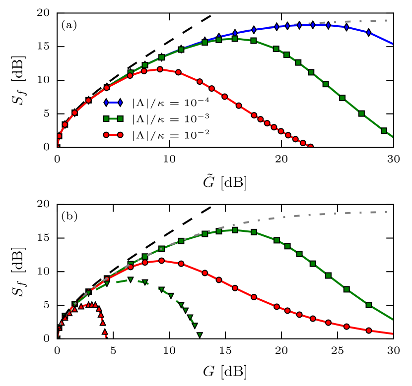
Fig. 10(a) shows the filtered squeezing level as a function of phase-preserving gain for a JPA with Kerr correction. For an ideal JPA, the squeezing level of the center frequency (Dirac-delta filtering) increases with gain without bound (dashed black curve). On the other hand, even for an ideal JPA (no higher-order corrections), the filtered squeezing level saturates for a finite-bandwidth filter (dotted-dashed gray curve). Indeed, as the gain increases, the squeezing bandwidth is reduced and eventually becomes smaller than the filter bandwidth. At that point, non-squeezed radiation contributes to limiting the measured squeezing level. This is a different illustration of the gain-bandwidth trade-off of cavity-based parametric amplifiers Clerk et al. (2010). A more detailed discussion of this effect is given in Appendix F. The three remaining curves show the effect of the Kerr nonlinearity on as a function of the numerically calculated gain [vertical axis of Fig. 5(a)]. As expected, while at low gain all curves overlap, for increasing gain reaches a maximal value, which decreases with Kerr nonlinearity.
Fig. 10(b) compares the squeezing level of a monochromatic current-pumped JPA (up and down triangles), and a bichromatic current-pumped JPA or monochromatic flux-pumped JPA (circle and squares) for two Kerr nonlinearities. As already discussed in Sec. V, the effect of nonidealities on the gain could not be obtained in the case of the monochromatic current-pumped JPA. To compare pumping schemes on equal footing, squeezing levels are shown as a function of the phase-preserving photon number gain calculated for an ideal DPA using Eq. (8). Note that the solid curves for the bichromatic current-pumped JPA present the same squeezing levels as in panel (a), but as a function of the ideal DPA gain. The curves have similar shapes for both pumping schemes. However, due to the additional cubic corrections, the monochromatic current pump JPA achieves smaller maximal squeezing level than is possible for a bichromatic current pump JPA with single Kerr-type correction. Hence, for the same JPA, going from a monochromatic to a bichromatic current pump allows to significantly increase the maximal squeezing level that can be produced. These results are in agreement with what could be expected from intracavity signatures in Sec. IV, where both the second order moments and the Wigner functions presented stronger nonidealities in the monochromatic current pump case.
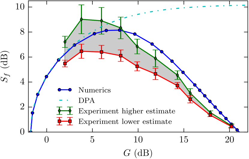
In order to confirm that these higher-order correction effects explain the experimentally observed reduction in squeezing levels of JPAs Castellanos-Beltran et al. (2008); Mallet et al. (2011); Murch et al. (2013b); Zhong et al. (2013), we compare our numerical results to experimental data. Using a moment-based reconstruction method, the squeezing level of a flux-pumped JPA is measured da Silva et al. (2010); Eichler et al. (2011); Menzel et al. (2012). Fig. 11 shows experimental results and numerical data together. The reconstruction technique being highly sensitive to the gain of the measurement chain, the green diamonds (red squares) are the higher (lower) estimate of the squeezing level based on the corresponding measurement chain gain estimate, while the error bars corresponds to statistical error evaluation. The blue circles are numerical results where all parameters of the simulations were obtained from independent experiments with no fitting parameters. As a comparison, the dotted-dashed light-blue line indicates the result expected for an ideal DPA. While there is quantitative agreement between numerics and experiment for the maximal squeezing level measured, the overall agreement is only qualitative. The small discrepancies could be due to spatial variations in the impedance of the JPA environment that leads to an experimentally observed variation in the gain-bandwidth product of the JPA with increasing gain.
We note that, contrary to previous hypothesis Zhong et al. (2013), our results indicate that the squeezing saturation happens at pump powers below the bifurcation threshold of the JPA. Our results strongly indicate the JPA higher-order correction as the main contributing factor to the experimentally observed decrease of squeezing in the large gain limit.
VI.3 Cumulants
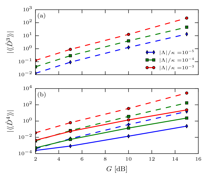
The Wigner functions of Fig. 4 clearly indicate that the higher-order corrections lead to non-Gaussian intracavity fields. In order to characterize the non-gaussianity of the filtered output field, we compute third and fourth order cumulants and . In the case of a univariate distribution, the third (fourth) order cumulant can be normalized to define the skew (kurtosis) of the distribution. While such definitions are not as straightforward in the case of the multivariate distribution considered here, the third and fourth order cumulants still characterize the non-Gaussian character of the field. Indeed, recall that a cumulant of order is a polynomial of moments of order and less, and that, for a Gaussian field, only the cumulants of order one and two are non-zero Puri (2001).
Fig. 12(a) shows numerical calculation of for the JPA with a monochromatic current pump. The cumulant increases following a power law with gain and nonlinearity. The numerical results for the bichromatic current and flux pump are not shown here as they are exactly zero. Fig. 12(b) shows a fourth order cumulant for both type of corrections. Again, in agreement with the results of Fig. 4, non-gaussianity increases with gain and nonlinearity. In addition, we observe that the slope is larger for the monochromatic current pump (cubic corrections). The other third and fourth order cumulants , , and were also calculated and similar trends were observed (data not shown).
These numerical results present higher-order corrections to the DPA Hamiltonian as a significant source of non-gaussianity in the output field. In addition to the experimental data presented below, these corrections could explain previously reported experimental observation of non-Gaussian features for JPAs Mallet et al. (2011); Zhong et al. (2013).
VI.4 Output field imaging

In order to further investigate the non-Gaussian features discussed above, we experimentally image the Husimi -function of the output field of a flux-driven JPA. A deconvolution technique is used to extract the JPA output field from the noisy histograms resulting from sampling the measurement chain output via homodyne detection. This methodology not only provides an experimental analysis of the higher-order cumulants of the output field but also provides a direct image of the output field that can be compared with qualitative expectations based on the intracavity fields calculated in Fig. 4. See Appendix D for experimental details of the method.
Fig. 13 presents a comparison of the output field for low JPA gain (5 dB, top row) and high JPA gain (24 dB, bottom row). In the figures, both the raw noisy histograms, which are the convolution of the signal with noise due to the amplification chain (left column), and the Husimi -function extracted through the use of deconvolutions (right column) are shown. In addition, panel (e) presents the magnitude of the cumulants up to fourth order extracted from the deconvolved distributions of panels (b) and (d). As expected from the numerical calculations, the low gain -function appears Gaussian up to experimental resolution and third and fourth order cumulants are small. On the contrary, the -function at high gain is non-Gaussian with a noticeable “S”-shaped distortion, consistent with expectations based on the intracavity fields presented in Figure 4 and also consistent with a recent semi-classical analysis of the JPA response Bienfait et al. (2016). The inferred third and fourth order output field cumulants presented in panel (e) clearly deviate from the ideal value of zero expected for a Gaussian distribution. However, from the numerical results of Figure 12 and the symmetry with respect to the centroid of the -function in panel (d), one would expect the role of the third order cumulants to be small. To this end, we note that the third order cumulants are smaller than the second order cumulants, in support of the numerical predictions and the imaged -functions.
To conclude, our experimental results are consistent with the numerically calculated intracavity Wigner functions presented in Fig. 4. While the different orientations of the squeezed ellipse relative to the axes is a consequence of different pump phases, the different orientations relative to the ellipse of the “S”-like nonideality for the numerically computed intracavity field and the measured output field is explained by input-output theory.
VII Conclusion
In summary, the Kerr-type nonlinear correction is a limiting factor for the measurement quantum efficiency of JPAs and the squeezing level of their output field. This correction also leads to non-Gaussian signatures observed both in the intracavity field Wigner function and the fourth order cumulants of the output field. Our combined numerical and experimental results allow to explain a broad range of experimental observations, such as the smaller than expected quantum efficiency of the JPA Murch et al. (2013a, b); Vijay et al. (2012); Weber (2014), the saturation and decrease of squeezing at high gain in JPAs Zhong et al. (2013); Murch et al. (2013b); Mallet et al. (2011); Castellanos-Beltran et al. (2008), and non-Gaussian signatures of the output field Zhong et al. (2013); Mallet et al. (2011). In particular, this work presents a new experimental characterization of the output field of a flux-driven JPA, as well as a direct experimental imaging of the non-Gaussian distortions of the output field. In addition, we have derived and compared the higher-order corrections to the JPA Hamiltonian for three different pumping schemes. Our work shows that, in addition to a Kerr-type quartic correction, cubic terms in the Hamiltonian are important in the case of the monochromatic current pump. These additional corrections lead to larger deviations from the expected DPA behavior such as lower attainable squeezing levels and larger non-Gaussian signatures.
In short, our results indicate three pathways to improving the performance of the JPA as a squeezer and amplifier. First, in the case of a JPA operated with a monochromatic current pump, moving instead to a bichromatic current pumping scheme eliminates cubic corrections, leading to a greatly increased maximal squeezing level and reduced non-Gaussian signatures. Remarkably, this improvement can be obtained for the same circuit and parameters. Otherwise, at the cost of a small added circuit complexity, but using only a single drive, flux pumping offers similar advantages. Second, our results illustrate clearly the value of designing JPAs with small Kerr nonlinearities. This can be obtained by using SQUID arrays to dilute the nonlinearity Castellanos-Beltran and Lehnert (2007); Eichler and Wallraff (2014) or adding additional linear inductance Zhou et al. (2014). Finally, our work emphasizes the phase-sensitivity of the JPA in the high gain regime, and the importance of fully characterizing the phase and frequency dependence of the gain matrix in order to operate at the optimal phases and frequencies where the effects of nonidealities are minimal.
In complement to the numerical approach considered in this paper, a better understanding of the higher-order corrections discussed might be obtained by considering analytical perturbation theory techniques Zhang et al. (2014). Preliminary results are promising Boutin (2015). Similar analysis for a Josephson junction based traveling-wave parametric amplifier could help the current experimental and theoretical effort Yaakobi et al. (2013); O’Brien et al. (2014); White et al. (2015); Grimsmo and Blais (2017); Macklin et al. (2015). Finally, while higher-order corrections hinder the performance of the JPA for squeezing and amplification, it can become a feature for other applications of the JPA such as robust cat state preparation and stabilization Puri et al. (2017a) which can be used for quantum computation Ofek et al. (2016) and quantum annealing Puri et al. (2017b).
Acknowledgements.
We thank A. A. Clerk, N. Didier, A. Kamal and M. H. Devoret for fruitful discussions. This work was supported by the Army Research Office under Grant W911NF-14-1-0078, FRQ-NT and NSERC. A.W.E. acknowledges support from the US Department of Defense through the NDSEG fellowship program. Computations were made on the supercomputer Mammouth parallele II from Université de Sherbrooke, managed by Calcul Québec and Compute Canada. The operation of this supercomputer is funded by the Canada Foundation for Innovation (CFI), NanoQuébec, RMGA and the Fonds de recherche du Québec - Nature et technologies (FRQ-NT). This research was undertaken thanks in part to funding from the Canada First Research Excellence Fund.Appendix A Solution to the DPA’s input-output equations
For this work to be self-contained, we present the standard solution to the equation of motions of the DPA discussed in Sec. II Collett and Gardiner (1984); Gardiner and Zoller (2004). Starting from Eq. (3) and introducing the vectors
| (56) |
the DPA can be described by the system of linear equations
| (57) |
where the matrix is
| (58) |
This system of linear equations is solved by introducing the Fourier transformed operator
| (59) |
We note that the Fourier transform of the creation operator is related to the adjoint of by . Thus, the solution to the linearized equations of motions in Fourier space is Collett and Gardiner (1984); Gardiner and Zoller (2004)
| (60) |
Using the input-output boundary condition Eq. (4), this result leads to Eq. (5) of the main text.
For completeness, we obtain from this expression the general expressions for the second order centered moments of the intracavity field used in Sec. IV
| (61) | ||||
| (62) |
Using the input-output boundary condition Eq. (4), the output field spectrums are Collett and Gardiner (1984)
| (63) | ||||
| (64) |
with , and similarly . These expressions allows to calculate analytically the DPA filtered output field spectrums presented in Sec. VI.
Appendix B Details of the displacement transformations
In this appendix, we detail the displacement transformations used to derive the Hamiltonian Eq. (16) for the monochromatic current-pumped JPA and the Hamiltonian Eq. (22) for the bichromatic current-pumped JPA. The unitary displacement transformation is Walls and Milburn (2008)
| (65) |
with , , and scalar complex numbers.
Applying this transformation on the driven Kerr Hamiltonian
| (66) |
with the detuning between the cavity and the rotating frame frequency, one obtains
| (67) |
Dropping constant terms and taking to emphasize the frame change, one obtains the Hamiltonian
| (68) |
where the linear pump term has been canceled by choosing the displacement parameter such that
| (69) |
The additional term originates from applying the displacement transformation on the master equation Eq. (35) instead of only the Hamiltonian.
In the single current-pump case of Sec. III.2, in a frame rotating at the pump frequency () the pump is simply , and one obtains the results of the main text by taking .
In the double pump case of Sec. III.3, in a frame rotating at the average pump frequency , the driving term is
| (70) |
with the detuning between the pumps . Inserting Eq. (70) in Eq. (69) and taking the ansatz leads to the coupled nonlinear differential equations
| (71) | ||||
| (72) | ||||
and to the Hamiltonian of Eq. (22). For , we can neglect the rotating terms under the RWA.
Since the parametric resonance condition only depends on the sum of the pump frequencies, and the amplitude of the classical field is bounded by the parametric threshold, one can choose in order to enforce the validity of the RWA. Under this approximation, the equations are the same as Eq. (18) in the monochromatic current pump case except that the equations are coupled through the frequency shift induced by the cavity population at both pump frequencies.
Appendix C Expansion of the flux-modulated Josephson energy
In this appendix, we complement Sec. III.4 by giving the analytical expressions for the Fourier coefficients of the Josephson energy of a flux modulated SQUID used in Eq. (29). Using the Jacobi-Anger formula Arfken and Weber (2005)
| (73) |
where is the Bessel function of the first kind, one obtains the Fourier coefficients
| (74) | ||||
| (75) | ||||
| (76) |
with .
In the case of a small amplitude flux pump (), the Bessel functions can be expanded. The leading term of each coefficient is such that
| (77) |
More explicitly, the first three coefficients of the Fourier expansion are, to leading order in ,
| (78) | ||||
| (79) | ||||
| (80) |
in agreement with the expressions of Refs. Wustmann and Shumeiko (2013); Krantz et al. (2013).
Appendix D Experimental setup and methods
This appendix presents details of the experimental setup and techniques used to obtain the experimental data for a flux-driven JPA presented in Figs. 11 and 13.
D.1 Experimental setup
We focus our characterization on an aluminum, lumped-element JPA. This design is of particular interest as it has been widely adopted for superconducting qubit readout Vijay et al. (2011); Mutus et al. (2013); Murch et al. (2013a). The device consists of a capacitance (3.2 pF) shunted by a SQUID ( = 45 pH). From simulations we estimate the geometric inductance of our design is 35 pH leading to a participation ratio . From these we estimate a Kerr nonlinearity MHz and from gain-bandwidth measurements a cavity damping rate MHz. This empirical value of is lower than expected from the lumped-element capacitance; we attribute this difference to spatial impedance variations in the JPA environment Mutus et al. (2014). The SQUID is flux-pumped to provide up to 25 dB of gain using an on-chip bias line Yamamoto et al. (2008) and the device is mounted with a 180∘ hybrid launch to reject common mode noise. The amplifier is shielded by an aluminum box and mounted at the base plate of a dilution refrigerator ( 20 mK). The signal from the JPA is further amplified with a commercial HEMT amplifier at 4K and subsequent room temperature amplifiers before being downconverted and digitized in a homodyne measurement.
The homodyne measurement samples the values of the conjugate quadrature components and described by the complex quadrature operator da Silva et al. (2010). For each measurement we averaged 256 consecutive voltage samples acquired at 1 GS/s, effectively filtering so as to analyze only highly-squeezed spectral components near the cavity frequency. The flux pump at frequency 2 is generated using a frequency doubler and the same microwave source that produces the local oscillator tone for the homodyne setup, allowing for good phase stability over the course of extended measurements. In addition, the JPA is hooked up to a switch on the base stage of the dilution refrigerator. The other port of the switch connects to a qubit dispersively coupled to a tunable resonator Ong et al. (2011). Through measurements of the qubit Stark shift, this setup enables a precise calibration of the power gain between the JPA and the ADC Macklin et al. (2015), a necessary input for our analysis.
D.2 Single-path reconstruction method
To characterize the properties of the output field we utilize the single path reconstruction method developed by Eichler et al. Eichler et al. (2011). We construct two histograms of , corresponding to the distribution with the JPA pump on, , and to the distribution with the JPA pump off, . We interleave the two measurements to mitigate the effects of experimental drift. We analyze the moments of the two histograms, and , to infer the normally-ordered moments of the output field, , through the expressions:
| (81) |
and
| (82) |
Here is the gain of the measurement chain between the JPA output and the ADC in the photon number basis Menzel et al. (2012); Menzel (2013) and is an effective noise mode dominated by the added noise of the HEMT amplifier. Experimentally, the power gain of the measurement chain was measured to be between 100.1 dB and 100.5 dB. These bounds on the power gain are reflected in the systematic uncertainty in the squeezing levels presented in Figure 11. Note that Eq. 82 is a limiting case of Eq. 81 when the JPA pump is off and is in the vacuum state. We iteratively solve these equations to compute the moments of the JPA output field and also quantify the cumulants of the output field, denoted by . For Gaussian states, such as ideal squeezed states, the cumulants are zero for . At each gain setting we histogram noise measurements which provides sufficient resolution to infer the field moments up to fourth order.
D.3 Imaging the output field using deconvolutions
To directly image the distortions of the output field due to nonidealities, we implement a complementary analysis technique based on applying series of deconvolutions to and . This method relies on the fact that these discrete distributions can be approximated as a convolution of quasi-probability distributions for the JPA output field and an effective noise mode of the measurement chain Kim (1997):
| (83) |
and
| (84) |
Here , , and are Husimi and Glauber-Sudarshan representations that describe the JPA output field, the vacuum state, and the noise mode Eichler et al. (2012). Given that the function can be obtained from the Wigner function via a Gaussian smoothing filter, we expect the distortions imaged by this deconvolution technique to be characteristic of both phase-space representations.
To reconstruct the output field, we first deconvolve with to obtain and then deconvolve with to obtain . Both deconvolutions are performed in Matlab using the Lucy-Richardson method Biggs and Andrews (1997). For the measurements in Figure 13, the power gain of the measurement chain was increased by 5 dB relative to the bounds quoted in Appendix D.2. We empirically found this larger gain led to improved resolution of the low-density tails of the output field Q functions. In all cases, inferences of the output field cumulants obtained via the moment-based reconstruction agreed with inferences of the cumulants calculated from the Q functions.
Appendix E Numerical calculation of filtered moments
In Sec. VI, we calculate moments of the filtered output field. Here, we give the details of the numerical technique used to obtain the results presented there. As an illustration of the technique, we consider the third order moment
| (85) |
with the three-times correlation function
| (86) | ||||
where the last equality is valid for a vacuum input field Gardiner and Collett (1985).
In order to use the quantum regression formula, we separate the integral in a sum over all possible time-orderings
| (87) | ||||
where, using the invariance under time-translation for a steady-state and assuming a purely real filter, we have defined
| (88) |
Finally, we integrate over each correlation function that we calculate using the general formula of the quantum regression result Gardiner and Zoller (2004). For the three-time correlation function, we obtain
| (89) | ||||
with the evolution superoperator from to , and . Numerically, the evolution is performed by integrating the master equation using the Runge-Kutta solver of the GSL numerical library Galassi et al. (2011).
Appendix F Squeezing level of the filtered DPA output field
In addition to the numerical approach of Appendix E, the results of Figs. 10 and 11 for the DPA can be obtained more simply by integrating the analytical expressions of Eqs. (63) and (64) using
| (90) | |||
| (91) |
with the Fourier transform of a real time-domain filter function . In particular, in the case of Fig. 10 where and , the minimal variance of the filtered output field is
| (92) |
As mentioned in the main text, the integrand is minimal (maximal squeezing) at the center frequency , and will increase (reduced squeezing) away from this frequency. Thus, as discussed in Sec. VI.2, the minimal variance of the filtered field will always be equal, or larger than, the variance at the center frequency. This limits the squeezing level of the JPA filtered output field, even without any nonidealities.
To further illustrate this effect, we consider the case of a narrow-band filter centered at frequency such that . In that case, the squeezing level is
| (93) |
which only diverges for , and otherwise reaches a finite maximal value of even at the parametric threshold. Neglecting the constant background, the half-width at half maximum of is , which will decrease with increasing gain reaching zero at the parametric threshold. This is a different illustration of the gain-bandwidth trade-off of cavity-based parametric amplifiers Clerk et al. (2010).
References
- Yurke et al. (1988) B. Yurke, P. G. Kaminsky, R. E. Miller, E. A. Whittaker, A. D. Smith, A. H. Silver, and R. W. Simon, Phys. Rev. Lett. 60, 764 (1988).
- Yurke et al. (1989a) B. Yurke, P. Kaminsky, R. Miller, E. Whittaker, A. Smith, A. Silver, and R. Simon, IEEE Transactions on Magnetics 25, 1371 (1989a).
- Yurke et al. (1989b) B. Yurke, L. R. Corruccini, P. G. Kaminsky, L. W. Rupp, A. D. Smith, A. H. Silver, R. W. Simon, and E. A. Whittaker, Phys. Rev. A 39, 2519 (1989b).
- Castellanos-Beltran and Lehnert (2007) M. A. Castellanos-Beltran and K. W. Lehnert, Applied Physics Letters 91, 083509 (2007).
- Yamamoto et al. (2008) T. Yamamoto, K. Inomata, M. Watanabe, K. Matsuba, T. Miyazaki, W. D. Oliver, Y. Nakamura, and J. S. Tsai, Applied Physics Letters 93, 042510 (2008).
- Bergeal et al. (2010) N. Bergeal, F. Schackert, M. Metcalfe, R. Vijay, V. Manucharyan, L. Frunzio, D. Prober, R. Schoelkopf, S. Girvin, and M. Devoret, Nature 465, 64 (2010).
- Hatridge et al. (2011) M. Hatridge, R. Vijay, D. H. Slichter, J. Clarke, and I. Siddiqi, Phys. Rev. B 83, 134501 (2011).
- Mutus et al. (2013) J. Y. Mutus, T. C. White, E. Jeffrey, D. Sank, R. Barends, J. Bochmann, Y. Chen, Z. Chen, B. Chiaro, A. Dunsworth, J. Kelly, A. Megrant, C. Neill, P. J. J. O’Malley, P. Roushan, A. Vainsencher, J. Wenner, I. Siddiqi, R. Vijay, A. N. Cleland, and J. M. Martinis, Applied Physics Letters 103, 122602 (2013).
- Eichler and Wallraff (2014) C. Eichler and A. Wallraff, EPJ Quantum Technology 1, 2 (2014).
- Mutus et al. (2014) J. Y. Mutus, T. C. White, R. Barends, Y. Chen, Z. Chen, B. Chiaro, A. Dunsworth, E. Jeffrey, J. Kelly, A. Megrant, C. Neill, P. J. J. O’Malley, P. Roushan, D. Sank, A. Vainsencher, J. Wenner, K. M. Sundqvist, A. N. Cleland, and J. M. Martinis, Applied Physics Letters 104, 263513 (2014).
- Eichler et al. (2014) C. Eichler, Y. Salathe, J. Mlynek, S. Schmidt, and A. Wallraff, Phys. Rev. Lett. 113, 110502 (2014).
- Jeffrey et al. (2014) E. Jeffrey, D. Sank, J. Y. Mutus, T. C. White, J. Kelly, R. Barends, Y. Chen, Z. Chen, B. Chiaro, A. Dunsworth, A. Megrant, P. J. J. O’Malley, C. Neill, P. Roushan, A. Vainsencher, J. Wenner, A. N. Cleland, and J. M. Martinis, Phys. Rev. Lett. 112, 190504 (2014).
- Vijay et al. (2011) R. Vijay, D. H. Slichter, and I. Siddiqi, Phys. Rev. Lett. 106, 110502 (2011).
- Castellanos-Beltran et al. (2008) M. Castellanos-Beltran, K. Irwin, G. Hilton, L. Vale, and K. Lehnert, Nature Physics 4, 929 (2008).
- Mallet et al. (2011) F. Mallet, M. A. Castellanos-Beltran, H. S. Ku, S. Glancy, E. Knill, K. D. Irwin, G. C. Hilton, L. R. Vale, and K. W. Lehnert, Phys. Rev. Lett. 106, 220502 (2011).
- Fedorov et al. (2016) K. G. Fedorov, L. Zhong, S. Pogorzalek, P. Eder, M. Fischer, J. Goetz, E. Xie, F. Wulschner, K. Inomata, T. Yamamoto, Y. Nakamura, R. Di Candia, U. Las Heras, M. Sanz, E. Solano, E. P. Menzel, F. Deppe, A. Marx, and R. Gross, Phys. Rev. Lett. 117, 020502 (2016).
- Murch et al. (2013a) K. Murch, S. Weber, C. Macklin, and I. Siddiqi, Nature 502, 211 (2013a).
- Weber et al. (2014) S. Weber, A. Chantasri, J. Dressel, A. Jordan, K. Murch, and I. Siddiqi, Nature 511, 570 (2014).
- Campagne-Ibarcq et al. (2014) P. Campagne-Ibarcq, L. Bretheau, E. Flurin, A. Auffèves, F. Mallet, and B. Huard, Phys. Rev. Lett. 112, 180402 (2014).
- Stehlik et al. (2015) J. Stehlik, Y.-Y. Liu, C. M. Quintana, C. Eichler, T. R. Hartke, and J. R. Petta, Phys. Rev. Applied 4, 014018 (2015).
- Virally et al. (2016) S. Virally, J. O. Simoneau, C. Lupien, and B. Reulet, Phys. Rev. A 93, 043813 (2016).
- Simoneau et al. (2017) J. O. Simoneau, S. Virally, C. Lupien, and B. Reulet, Phys. Rev. B 95, 060301 (2017).
- Goetz et al. (2017) J. Goetz, S. Pogorzalek, F. Deppe, K. G. Fedorov, P. Eder, M. Fischer, F. Wulschner, E. Xie, A. Marx, and R. Gross, Phys. Rev. Lett. 118, 103602 (2017).
- Caves (1982) C. Caves, Phys. Rev. D 26, 1817 (1982).
- Roy and Devoret (2016) A. Roy and M. Devoret, Comptes Rendus Physique 17, 740 (2016).
- Walls and Milburn (2008) D. Walls and G. Milburn, Quantum Optics, SpringerLink: Springer e-Books (Springer, 2008).
- Gardiner and Zoller (2004) C. Gardiner and P. Zoller, Quantum Noise: A Handbook of Markovian and Non-Markovian Quantum Stochastic Methods with Applications to Quantum Optics, Springer Series in Synergetics (Springer, 2004).
- Zhong et al. (2013) L. Zhong, E. P. Menzel, R. D. Candia, P. Eder, M. Ihmig, A. Baust, M. Haeberlein, E. Hoffmann, K. Inomata, T. Yamamoto, Y. Nakamura, E. Solano, F. Deppe, A. Marx, and R. Gross, New Journal of Physics 15, 125013 (2013).
- Murch et al. (2013b) K. Murch, S. Weber, K. Beck, E. Ginossar, and I. Siddiqi, Nature 499, 62 (2013b).
- Bienfait et al. (2016) A. Bienfait, P. Campagne-Ibarcq, A. Holm-Kiilerich, X. Zhou, S. Probst, J. J. Pla, T. Schenkel, D. Vion, D. Esteve, J. J. L. Morton, K. Moelmer, and P. Bertet, ArXiv e-prints (2016), arXiv:1610.03329 [cond-mat.mes-hall] .
- Vijay et al. (2012) R. Vijay, C. Macklin, D. Slichter, S. Weber, K. Murch, R. Naik, A. N. Korotkov, and I. Siddiqi, Nature 490, 77 (2012).
- Weber (2014) S. J. Weber, Quantum Trajectories of a Superconducting Qubit, Ph.D. thesis, University of California, Berkeley (2014).
- Yurke and Buks (2006) B. Yurke and E. Buks, Lightwave Technology, Journal of 24, 5054 (2006).
- Kamal et al. (2009) A. Kamal, A. Marblestone, and M. Devoret, Phys. Rev. B 79, 184301 (2009).
- Wustmann and Shumeiko (2013) W. Wustmann and V. Shumeiko, Phys. Rev. B 87, 184501 (2013).
- Zhou et al. (2014) X. Zhou, V. Schmitt, P. Bertet, D. Vion, W. Wustmann, V. Shumeiko, and D. Esteve, Phys. Rev. B 89, 214517 (2014).
- Eichler (2013) C. Eichler, Experimental Characterization of Quantum Microwave Radiation, Ph.D. thesis, ETH Zurich (2013).
- Kochetov and Fedorov (2015) B. A. Kochetov and A. Fedorov, Phys. Rev. B 92, 224304 (2015).
- Laflamme and Clerk (2011) C. Laflamme and A. A. Clerk, Phys. Rev. A 83, 033803 (2011).
- Landau and Lifshitz (1969) L. Landau and E. Lifshitz, Mechanics, second edition ed., vol. 1 (Pergamon Press, 1969).
- Nation et al. (2012) P. D. Nation, J. R. Johansson, M. P. Blencowe, and F. Nori, Rev. Mod. Phys. 84, 1 (2012).
- Collett and Gardiner (1984) M. J. Collett and C. W. Gardiner, Phys. Rev. A 30, 1386 (1984).
- Wilson et al. (2010) C. M. Wilson, T. Duty, M. Sandberg, F. Persson, V. Shumeiko, and P. Delsing, Phys. Rev. Lett. 105, 233907 (2010).
- Bourassa et al. (2012) J. Bourassa, F. Beaudoin, J. M. Gambetta, and A. Blais, Phys. Rev. A 86, 013814 (2012).
- Koch et al. (2007) J. Koch, T. M. Yu, J. Gambetta, A. A. Houck, D. I. Schuster, J. Majer, A. Blais, M. H. Devoret, S. M. Girvin, and R. J. Schoelkopf, Physical Review A 76 (2007).
- Leib et al. (2012) M. Leib, F. Deppe, A. Marx, R. Gross, and M. J. Hartmann, New Journal of Physics 14, 075024 (2012).
- Manucharyan et al. (2007) V. E. Manucharyan, E. Boaknin, M. Metcalfe, R. Vijay, I. Siddiqi, and M. Devoret, Phys. Rev. B 76, 014524 (2007).
- Devoret (1995) M. H. Devoret, Les Houches, Session LXIII (1995).
- Barnett and Radmore (1997) S. Barnett and P. Radmore, Methods in Theoretical Quantum Optics, Oxford science publications (Clarendon Press, 1997).
- Krantz et al. (2013) P. Krantz, Y. Reshitnyk, W. Wustmann, J. Bylander, S. Gustavsson, W. D. Oliver, T. Duty, V. Shumeiko, and P. Delsing, New Journal of Physics 15, 105002 (2013).
- Tinkham (2004) M. Tinkham, Introduction to Superconductivity: Second Edition, Dover Books on Physics (Dover Publications, 2004).
- Dodonov and Man’ko (2003) V. Dodonov and V. Man’ko, Theory of Nonclassical States of Light (Taylor & Francis, 2003).
- Wilson-Gordon et al. (1991) A. D. Wilson-Gordon, V. Buek, and P. L. Knight, Phys. Rev. A 44, 7647 (1991).
- Kirchmair et al. (2013) G. Kirchmair, B. Vlastakis, Z. Leghtas, S. E. Nigg, H. Paik, E. Ginossar, M. Mirrahimi, L. Frunzio, S. Girvin, and R. Schoelkopf, Nature 495, 205 (2013).
- Liu et al. (2017) G. Liu, T.-C. Chien, X. Cao, O. Lanes, E. Alpern, D. Pekker, and M. Hatridge, ArXiv e-prints (2017), arXiv:1703.04425 [quant-ph] .
- Leonhardt and Paul (1994) U. Leonhardt and H. Paul, Phys. Rev. Lett. 72, 4086 (1994).
- Pozar (1997) D. Pozar, Microwave Engineering (Wiley, 1997).
- Eichler et al. (2011) C. Eichler, D. Bozyigit, C. Lang, L. Steffen, J. Fink, and A. Wallraff, Phys. Rev. Lett. 106, 220503 (2011).
- da Silva et al. (2010) M. P. da Silva, D. Bozyigit, A. Wallraff, and A. Blais, Phys. Rev. A 82, 043804 (2010).
- Clerk et al. (2010) A. A. Clerk, M. H. Devoret, S. M. Girvin, F. Marquardt, and R. J. Schoelkopf, Rev. Mod. Phys. 82, 1155 (2010).
- Menzel et al. (2012) E. P. Menzel, R. Di Candia, F. Deppe, P. Eder, L. Zhong, M. Ihmig, M. Haeberlein, A. Baust, E. Hoffmann, D. Ballester, K. Inomata, T. Yamamoto, Y. Nakamura, E. Solano, A. Marx, and R. Gross, Phys. Rev. Lett. 109, 250502 (2012).
- Puri (2001) R. Puri, Mathematical Methods of Quantum Optics, Physics and astronomy online library (Springer, 2001).
- Zhang et al. (2014) J. Zhang, Y.-x. Liu, R.-B. Wu, K. Jacobs, S. Kaya Ozdemir, L. Yang, T.-J. Tarn, and F. Nori, ArXiv e-prints (2014), arXiv:1407.8108 [quant-ph] .
- Boutin (2015) S. Boutin, Amplificateur paramétrique Josephson : Limite quantique, modélisation et caractérisation, Master’s thesis, Université de Sherbrooke (2015).
- Yaakobi et al. (2013) O. Yaakobi, L. Friedland, C. Macklin, and I. Siddiqi, Phys. Rev. B 87, 144301 (2013).
- O’Brien et al. (2014) K. O’Brien, C. Macklin, I. Siddiqi, and X. Zhang, Phys. Rev. Lett. 113, 157001 (2014).
- White et al. (2015) T. C. White, J. Y. Mutus, I.-C. Hoi, R. Barends, B. Campbell, Y. Chen, Z. Chen, B. Chiaro, A. Dunsworth, E. Jeffrey, J. Kelly, A. Megrant, C. Neill, P. J. J. O’Malley, P. Roushan, D. Sank, A. Vainsencher, J. Wenner, S. Chaudhuri, J. Gao, and J. M. Martinis, Applied Physics Letters 106, 242601 (2015).
- Grimsmo and Blais (2017) A. L. Grimsmo and A. Blais, npj Quantum Information 3, 20 (2017).
- Macklin et al. (2015) C. Macklin, K. O’Brien, D. Hover, M. E. Schwartz, V. Bolkhovsky, X. Zhang, W. D. Oliver, and I. Siddiqi, Science 350, 307 (2015).
- Puri et al. (2017a) S. Puri, S. Boutin, and A. Blais, npj Quantum Information 3, 18 (2017a).
- Ofek et al. (2016) N. Ofek, A. Petrenko, R. Heeres, P. Reinhold, Z. Leghtas, B. Vlastakis, Y. Liu, L. Frunzio, S. M. Girvin, L. Jiang, M. Mirrahimi, M. H. Devoret, and R. J. Schoelkopf, Nature 536, 441 (2016).
- Puri et al. (2017b) S. Puri, C. K. Andersen, A. L. Grimsmo, and A. Blais, Nature Comm. 8, 15785 (2017b).
- Arfken and Weber (2005) G. Arfken and H. Weber, Mathematical Methods For Physicists (Elsevier, 2005).
- Ong et al. (2011) F. R. Ong, M. Boissonneault, F. Mallet, A. Palacios-Laloy, A. Dewes, A. C. Doherty, A. Blais, P. Bertet, D. Vion, and D. Esteve, Phys. Rev. Lett. 106, 167002 (2011).
- Menzel (2013) E. Menzel, Ph.D. thesis, Technische Universität München (2013).
- Kim (1997) M. S. Kim, Phys. Rev. A 56, 3175 (1997).
- Eichler et al. (2012) C. Eichler, D. Bozyigit, and A. Wallraff, Phys. Rev. A 86, 032106 (2012).
- Biggs and Andrews (1997) D. S. C. Biggs and M. Andrews, Appl. Opt. 36, 1766 (1997).
- Gardiner and Collett (1985) C. W. Gardiner and M. J. Collett, Phys. Rev. A 31, 3761 (1985).
- Galassi et al. (2011) M. Galassi, J. Davies, J. Theiler, B. Gough, G. Jungman, P. Alken, M. Booth, and F. Rossi, “Gnu Scientific Library: Reference Manual,” (2011).