Perfect spin filter by periodic drive of a ferromagnetic quantum barrier

Abstract

We consider the problem of particle tunneling through a periodically driven ferromagnetic quantum barrier connected to two leads. The barrier is modeled by an impurity site representing a ferromagnetic layer or quantum dot in a tight-binding Hamiltonian with a local magnetic field and an AC-driven potential, which is solved using the Floquet formalism. The repulsive interactions in the quantum barrier are also taken into account. Our results show that the time-periodic potential causes sharp resonances of perfect transmission and reflection, which can be tuned by the frequency, the driving strength, and the magnetic field. We demonstrate that a device based on this configuration could act as a highly-tunable spin valve for spintronic applications.

The problem of a magnetic impurity embedded in a metallic matrix has been extensively studied over many years, particularly since the discovery of the Kondo effect Kondo_64 . The Kondo or sd model that captured the low-energy physics in the local moment regime of such systems was soon proved to be equivalent to the Anderson model Anderson_61 . In the early years, the main interest was focused on the thermodynamic properties of such systems, and analytical solutions Yosida.70 ; Yamada.75 ; Yamada.76 ; Yamada.79 ; Zlatic.83 as well as numerical methods such as numerical renormalization group Costi.94c ; Costi.10 have been extensively applied to deal with strong electronic correlations. More recently, the problem has recovered interest for its non-equilibrium and transport propertiesBeenakker.91 ; iftikhar2015two , particularly since the possibility to construct tunable impurities in experimental systems such as semiconductor quantum dots or single-molecule transistors became available GoldhaberGordon.98 ; Scott.09 ; Scott.13 ; perrin2015single .

The vast majority of the theoretical work related to the non-equilibrium problem considers the steady-state conductance as a function of a constant bias voltage Schiller.95 ; Majumdar.98 ; Oguri.01 ; Oguri.05 ; Hewson.05 ; Sela.09 ; Pletyukhov.12 and its universal aspects Doyon.06 . A more difficult, however exciting problem, arises when the system is subjected to a periodically driven potential.

Besides the solid state scenario, periodically driven tight-binding systems can be realized with optical lattices and cold atom systemsBloch_05 . These types of systems have provided an exciting scenario, not only as experimental simulations of solid-state models, but also to test configurations with potential new features Bloch_05 ; Zhang_014 ; Greschner_015 ; aidelsburger2015measuring ; douglas2015quantum ; ponte2015many ; ott14 ; shaking1 ; shaking2 ; agarwal17 ; PhysRevLett.118.260602 .

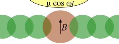
Figure 1: Schematic setup of a ferromagnetic quantum barrier subjected to a periodic drive and connected to two leads.

In this work, we study the transmission of electrons through a ferromagnetic quantum barrier with a driven gate potential and connected to two leads as illustrated in Fig. 1. We consider electronic excitations of opposite spin traveling along a tight-binding chain with nearest neighbor hopping amplitude $J$. A periodically driven gate with angular frequency $\omega$ and amplitude $\mu$ is imposed upon the quantum barrier at the central site together with a local magnetic field $B$. The possibility of a local electron-electron interaction of strength $U$ and a local potential energy $\epsilon_{d}$ on the barrier are also included. The resulting Hamiltonian reads ($\hbar=1$)

$$H = -J\sum_{i,\sigma}(c_{i,\sigma}^{\dagger}c_{i+1,\sigma}{\phantom{\dagger}}+c_{i+1,\sigma}^{\dagger}c_{i,\sigma}{\phantom{\dagger}})$$

$$+\sum_{\sigma}\left(\epsilon_{d}-\mu\cos(\omega t)-\sigma b\right)c_{0,\sigma}^{\dagger}c_{0,\sigma}{\phantom{\dagger}}+Un_{0,\uparrow}n_{0,\downarrow}$$

in standard notation where $b=\frac{\mu_{B}}{2}B$. It has been established that single particle transmission through a driven impurity without magnetic field can give rise to sharp resonances, where the transmission vanishes completely even for infinitesimally small driving amplitudes reyes2017transport ; thuberg2016quantum . We now show that the addition of a magnetic field and the local potential energy not only make the transmission spin-dependent but also cause an entirely new effect of perfect transmission for special parameters. The combination of such ballistic transmission and total reflection for different spin-dependent parameters therefore opens the possibility to construct a perfect spin filter, that may be very attractive for spintronics applications.

To calculate the transmission probability for each spin channel we will find steady-state solutions to the Schrödinger equation

$$(H(t)-i\partial_{t})\left|\Psi(t)\right>=0.$$ (2)

using the Floquet formalism Hanggi_98 for a time-periodic Hamiltonian of the form $H(t)=H_{0}+2H_{1}\cos(\omega t)$ as in Eq. (Perfect spin filter by periodic drive of a ferromagnetic quantum barrier). The steady-state solution is a so-called Floquet state $\left|\Psi(t)\right>=e^{-i\epsilon t}\left|\Phi(t)\right>$, which can be determined by the eigenvalue equation

$$(H(t)-i\partial_{t})\left|\Phi(t)\right>=\epsilon\left|\Phi(t)\right>.$$ (3)

where $\left|\Phi(t)\right>=\left|\Phi(t+2\pi/\omega)\right>$ is time-periodic and $\epsilon$ is the quasienergy. Using the spectral decomposition

$$|\Phi(t)\rangle=\sum_{n=-\infty}^{\infty}e^{-in\omega t}|\Phi_{n}\rangle,$$ (4)

the eigenvalue equation becomes

$$H_{0}|\Phi_{n}\rangle+H_{1}(|\Phi_{n+1}\rangle+|\Phi_{n-1}\rangle)=(\epsilon+n\omega)|\Phi_{n}\rangle.$$ (5)

The repulsive Coulomb interaction $U$ on the barrier induces many-body correlations, which are technically difficult to deal with even in thermal equilibrium. As we show in the Appendix I it is possible to develop a mean-field approach for Floquet systems by using a time-dependent density on the barrier $\langle n_{0,\sigma}\rangle$ such that $n_{0,\uparrow}n_{0,\downarrow}\approx\langle n_{0,\uparrow}\rangle n_{0,\downarrow}+\langle n_{0,\downarrow}\rangle n_{0,\uparrow}-\langle n_{0,\uparrow}\rangle\langle n_{0,\downarrow}\rangle$. In this way it is possible to use a general single particle state with spin $\sigma$, which is defined by the coefficients for all modes of the spectral decomposition

$$|\Phi_{n}^{\sigma}\rangle=\sum_{j}\phi^{\sigma}_{j,n}c_{j,\sigma}^{\dagger}|0\rangle,$$ (6)

where $|0\rangle$ is the vacuum state. Inserting Eq. (6) into the eigenvalue equation (3) results in recursion relations for the amplitudes $\phi_{j,n}$. For the bulk ($j\neq 0$) we have

$$-J(\phi^{\sigma}_{j-1,n}+\phi^{\sigma}_{j+1,n})=\bar{\epsilon}_{n,\sigma}\phi^{\sigma}_{j,n},$$ (7)

where

$$\bar{\epsilon}_{n,\sigma}=\epsilon+U\beta_{n,\sigma}+n\omega.$$ (8)

Here we have defined a mean-field parameter $\beta_{n,\sigma}=\sum_{m}\nu_{m,\sigma}\nu_{n-m,\bar{\sigma}}$ and $\nu_{m,\sigma}=\sum_{n}\phi^{\sigma\ *}_{0,n}\phi^{\sigma}_{0,n+m}$, where we have used the notation $\bar{\sigma}=-\sigma$. In contrast to ordinary mean field calculations, it is essential that the density on the driven quantum barrier is time-dependent (see Appendix I). This has the interesting consequence that all Floquet modes become coupled at the quantum barrier for $j=0$

$$- J(\phi^{\sigma}_{-1,n}+\phi^{\sigma}_{1,n})-\frac{\mu}{2}(\phi^{\sigma}_{0,n+1}+\phi^{\sigma}_{0,n-1})$$ (9)

$$+ U\sum_{m}\nu_{m,\bar{\sigma}}\phi^{\sigma}_{0,n-m}=(\bar{\epsilon}_{n}-\epsilon_{d}+\sigma b)\phi^{\sigma}_{0,n}.$$

The time-periodic potential in the quantum barrier is not energy conserving and can cause scattering into other Floquet modes $n$. For an incoming wave with wavenumber $k_{0}$ for the mode $n=0$ with quasi-energy $\bar{\epsilon}=-2J\cos k_{0}$, the solution of Eq. (7) has the form

$$|\Phi_{n}^{\sigma}\rangle = \sum_{j<0}\left[\delta_{n,0}Ae^{ik_{0}j}c_{j,\sigma}^{\dagger}+e^{-ik_{n}j}r_{n,\sigma}c_{j,\sigma}^{\dagger}\right]|0\rangle$$ (10)

$$+ \sum_{j>0}e^{ik_{n}j}t_{n,\sigma}c_{j,\sigma}^{\dagger}|0\rangle+E_{n,\sigma}c^{\dagger}_{0,\sigma}|0\rangle.$$

where the wavenumbers are given by $-2J\cos k_{n}=\bar{\epsilon}+n\omega$. If $|\bar{\epsilon}+n\omega|<2J$, $k_{n}$ is real and the corresponding plane wave solutions are delocalized over the entire chain (unbound channels), which is always the case for the incoming wave $n=0$. For modes with $\bar{\epsilon}+n\omega<-2J$, $k_{n}=i\kappa_{n}$ is imaginary and the solutions decay exponentially around the impurity (bound channels). For $\bar{\epsilon}+n\omega>2J$ the solutions decay and oscillate with a complex wavenumber $k_{n}=i\kappa_{n}+\pi$. Using Eq. (7) it is easy to check that

$$E_{n,\sigma}=t_{n,\sigma}=r_{n,\sigma}+\delta_{n,0}A,$$ (11)

capturing the inversion symmetry of the lattice with respect to $j=0$. Inserting the amplitudes $\phi_{j,n}^{\sigma}$ that arise after Eq. (11) back into Eq. (9), we obtain a recursive relation for the coefficients $E_{n,\sigma}$:

$$E_{n+1,\sigma}+E_{n-1,\sigma} = -\frac{4i\,J}{\mu}\sin k_{n}(E_{n,\sigma}-A\delta_{n,0})$$ (12)

$$+\frac{2}{\mu}U\gamma_{n}-\frac{2}{\mu}\sigma(b-{\sigma}\epsilon_{d})E_{n,\sigma},$$

which is the central equation that needs to be solved by requiring convergence $E_{|n|\to\infty}\to 0$. Here the influence of the interaction is captured by the term $\gamma_{n,\sigma}=\sum_{m}\nu_{m,\sigma}\phi^{\bar{\sigma}}_{0,n-m}$, which obviously depends on the total density of particles with opposite spin and can be iteratively determined self-consistently. In the following, we assume an unpolarized incoming current composed of equal amplitudes for opposite spin.

For the transmission coefficient, it is useful to observe that that the current of the incoming wave (normalized to $|A|^{2}\sin k_{0}$) has to equal the sum of all outgoing waves

$$\sum_{n}\left(|r_{n,\sigma}|^{2}+|t_{n,\sigma}|^{2}\right)\sin(k_{n})=A^{2}\sin(k_{0}).$$ (13)

Therefore, the total transmission can be expressed in terms of the solution for $E_{n,\sigma}$

$$T_{\sigma} = \frac{1}{A^{2}}\sum_{n}T_{n,\sigma}=\frac{1}{A^{2}}\sum_{n}|E_{n,\sigma}|^{2}\cdot\frac{\sin(k_{n})}{\sin(k_{0})}=\frac{{\rm Re}E_{0,\sigma}}{A}$$ (14)

$$= {\rm Re}\left[\frac{u_{k}}{u_{k}-\frac{i\mu}{2}\left(\frac{E_{1,\sigma}}{E_{0,\sigma}}+\frac{E_{-1,\sigma}}{E_{0,\sigma}}\right)-i\,\sigma\tilde{b}_{\sigma}}\right],$$

where we have used Eq. (12) for $n=0$ in the last line, with $u_{k}=2J\sin k_{0}$ as the incoming particle velocity and

$$\tilde{b}_{\sigma}=b-\sigma(\epsilon_{d}+U\gamma_{0,\sigma}/E_{0,\sigma}).$$ (15)

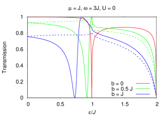
Figure 2: Transmission of both spin channels (solid line: spin up; dashed line: spin down) for a perturbation with $\omega=3J$, $\mu=J$ and various magnetic field strengths $b$ as function of $\epsilon$. The interaction is turned off ($U=0$) and $\epsilon_{d}=0$

.

Let us first consider the effect of a magnetic field $b$ without interactions $U=0$ and for vanishing on-site energy $\epsilon_{d}=0$, as shown in Fig. 2 as a function of incoming energy $-2J<\epsilon<2J$. Since the results are the same for $\epsilon\to-\epsilon$ and $\tilde{b}_{\sigma}\to-\tilde{b}_{\sigma}$, only the energy range of the upper half of the band is shown. Maybe the most striking features are the points of complete reflection $T=0$ at certain energies $\epsilon$. For $b=0$ these reflection points were linked to the phenomena of Fano resonances and are known to occur even for arbitrary small driving amplitudes $\mu\to 0$ at incoming energies $\epsilon\to\omega-2J$ thuberg2016quantum ; reyes2017transport . For $\sigma b<0$ there are no such resonances, but for $\sigma b>0$ the points of perfect reflection now shift to lower energies and we observe a new feature of perfect transmission at nearby incoming energies, which opens the possibilities to construct a perfect spin-filter as outlined below. To estimate the locations of the zero transmission resonances, it is instructive to consider the recurrence relation in Eq. (12) for $n\neq 0$, which can be written as $E_{n+1,\sigma}+E_{n-1,\sigma}=\alpha_{n}E_{n,\sigma}$ where

$$\alpha_{n}=\frac{2}{\mu}\left[-{\rm sign}{(n)}\sqrt{(\epsilon+n\omega)^{2}-4J^{2}}-\sigma\tilde{b}_{\sigma}\right].$$ (16)

For small driving amplitudes $\mu\to 0$ the $\alpha_{n}$ grow beyond bounds, but a resonance condition $E_{0,\sigma}/E_{-1,\sigma}\to 0$ in Eq. (14) is still possible for $\alpha_{-1}\to 0$, so that the points of zero transmission are given by

$$\epsilon\stackrel{{\scriptstyle\mu\to 0}}{{\longrightarrow}}\omega-\sqrt{4J^{2}+\tilde{b}_{\sigma}^{2}}$$ (17)

for $\sigma b>0$. As mentioned above there are corresponding resonances for $\epsilon\to-\epsilon$ and reversed spin (or field). However, if the frequency is too small or the field is too large so that the expression in Eq. (17) becomes negative, the resonances are pushed outside the band and there will be no points of zero transmission for any energy. On the other hand, for any given incoming energy $\epsilon$ in the band it is possible to find a sufficiently high frequency so that Eq. (17) can be fulfilled.

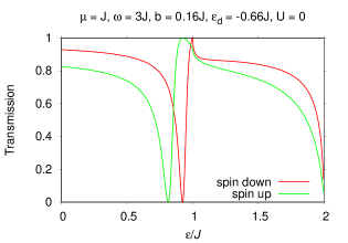
Figure 3: Transmission behavior of both spin channels for a perturbation with $\hbar\omega=3J$, $\mu=J$, a magnetic field strength $b=0.16J$ and a constant potential $\epsilon_{d}=-0.66J$ showing the possibility for a perfect spin filter.

The points of perfect transmission $T=1$ in Fig. 2 are also linked to the Fano resonance, which has been studied for static side coupled systems miroshnichenko2005engineering . In our case the effective magnetic field $\sigma\tilde{b}_{\sigma}$ in Eq.(15) leads to a finite Fano asymmetry parameter and therefore a nearby point of perfect transmission. Basically the reduced Zeeman energy enhances the local occupation at the impurity site and increases transmission through the barrier. This effect can also be achieved by a local potential energy $\epsilon_{d}$ as an additional tuning parameter. In particular, it is straight-forward to choose a negative value of $\epsilon_{d}$ and a small positive value of $b$, so that the effective on-site energy $\sigma\tilde{b}_{\sigma}$ is attractive for both spin-channels but resulting in a spin-dependent shift in Eq. (17). In Fig. 3 the parameters $b=0.16J$ and $\epsilon_{d}=-0.66J$ were chosen so that the transmission maximum for spin-up occurs at the same energy as the resonance of perfect reflection for spin-down. This demonstrates that it is possible to create a perfect spin-filter by a combination of a static magnetic field and a local time-periodic potential.

In the high frequency regime $\omega\gg J,\tilde{b}_{\sigma}$ the coefficients $\alpha_{n}$ in Eq. (16) can be expanded to first order in $\omega^{-1}$. The resulting (approximate) recurrence relation has an exact solution in terms of Bessel functions of the first kind $\mathcal{J}(x)$ thuberg2016quantum ; della2007visualization . Thus, in this regime we can obtain an analytical approximation for the transmission

$$T_{\sigma}\approx\frac{u_{k}^{2}}{u_{k}^{2}+\left(\frac{\mu}{2}\chi(\mu/\omega)+\sigma\tilde{b}_{\sigma}\right)^{2}},$$ (18)

where $\chi(\mu/\omega)=\frac{\mathcal{J}_{1-\epsilon/\omega-\sigma\tilde{b}_{\sigma}/\omega}(\mu/\omega)}{\mathcal{J}_{-\epsilon/\omega-\sigma\tilde{b}_{\sigma}/\omega}(\mu/\omega)}-\frac{\mathcal{J}_{1+\epsilon/\omega+\sigma\tilde{b}_{\sigma}/\omega}(\mu/\omega)}{\mathcal{J}_{\epsilon/\omega+\sigma\tilde{b}_{\sigma}/\omega}(\mu/\omega)}$. A comparison between this approximation and the exact result is shown in Fig. (4). Moreover, a first-order expansion of $\chi(\mu/\omega)$ in $\epsilon+\sigma\tilde{b}_{\sigma}$ leads to an analytical estimate for the location of the point of perfect transmission $T_{\sigma}=1$ at $\mathcal{J}_{0}(\mu/\omega)^{2}=\sigma\tilde{b}_{\sigma}/\epsilon+1$. We see that tuning of the resonance locations is therefore also equally possible by changing $\mu$ or $\omega$ and both calculations coincide almost perfectly already for $\omega=10J$.

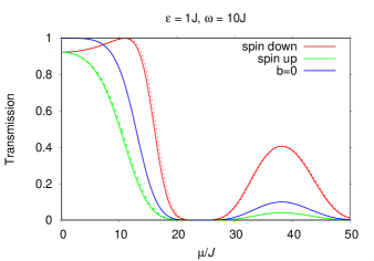
Figure 4: Transmission of both spin channels for a perturbation with $\omega=10J$ and a magnetic field of $b=0.5$ as function of $\mu$. The interaction is turned off ($U=0$) and $\epsilon_{d}=0$. The dashed lines correspond to the approximation from Eq. (18)

Last but not least the effect of interactions $U\neq 0$ must be considered. As can be seen from Eq. (15) the main effect comes from the renormalization of the effective magnetic field $\tilde{b}_{\sigma}$ by a spin-dependent contribution to the local potential energy $\epsilon_{d}+U\gamma_{0,\sigma}/E_{0,\sigma}$ in the mean field approximation. Therefore, a similar effect as seen in Fig. 3 is observed in this case, where two independent Fano resonances appear for each spin channel. The position of the resonances is approximately given by Eq. (17), with a small shift in comparison with the non-interacting case, which is self-consistently calculated within the mean-field approximation through the parameter $U\gamma_{0,\sigma}/E_{0,\sigma}$. We notice that at high frequency $\omega$ and small amplitudes $\mu$, the occupation of the Floquet coefficients $n\neq 0$ becomes negligible, and hence in this limit one has $U\gamma_{0,\sigma}/E_{0,\sigma}\sim U\langle n_{0,\sigma}\rangle$, such that the effective site energy is approximately $\epsilon_{d}+U\langle n_{0,\sigma}\rangle$, which is precisely the Hartree-Fock expression for a static impurity subject to a local interaction Hewson.93 ; Hewson . This is consistent with the interpretation following Eq. (18) that in the very high frequency regime, the oscillations average-out and the system can be effectively described by static fields and local potentialsreyes2017transport ; della2007visualization . In particular, using an effective field on the barrier $b_{\rm eff}=\tilde{b}_{\sigma}+\sigma\frac{\mu}{2}\chi(\mu/\omega)$ gives the same high frequency transmission coefficient $T=b_{\rm eff}^{2}/(u_{k}^{2}+b_{\rm eff}^{2})$, i.e. the local potential must simply be shifted by $\frac{\mu}{2}\chi$.

In conclusion, we have analyzed the effect of a local time-periodic potential on the transport through a ferromagnetic quantum barrier including local potentials, fields, and interactions. In contrast to static gating and filtering mechanisms, the periodic drive allows points of perfect transmission and complete reflection, which is useful for the generation of tunable spin-currents. To achieve complete reflection for spin-down and perfect transmission for spin-up as shown in Fig. 3, two parameters must be tuned, such as the local static potential and the driving frequency. The technological implementation of such a perfect spin filter requires relatively high frequencies of the order of the incoming energy, which is normally the Fermi-energy relative to the band edge. Therefore, systems with low filling, small hopping, or very heavy effective mass are most promising in this respect. The geometry of the setup is of course not limited to a quasi one-dimensional array with a central quantum dot shown in Fig. 1, since the effect can also be derived in the same way for any system where the transport channels go through a ferromagnetic layer with a tunable time-periodic potential.

I Appendix

Here we discuss in detail the mathematical formulation and intermediate steps leading to the mean-field theory approximation and corresponding Floquet equations presented in the main body of the article.

For a system that is periodically driven, periodicity in time allows to express the solutions to the dynamical problem in terms of a set of eigenfunctions $|\Psi(t)\rangle=e^{-i\hbar^{-1}\epsilon t}|\Phi(t)\rangle$, with $\epsilon$ a Floquet eigenvalue, and an associated periodic eigenfunction $|\Phi(t+T)\rangle=|\Phi(t)\rangle$. If one restricts the non-equivalent values of $\epsilon$ to a first Brillouin zone $\epsilon\in\left[-\pi\hbar/T,\pi\hbar/T\right]$, then the periodic eigenfunction can be expanded as

$$|\Phi(t)\rangle=\sum_{n\in Z}e^{-in\omega t}|\Phi_{n}\rangle,$$ (19)

where each stationary Floquet mode $|\Phi_{n}\rangle$ is associated to an eigenvalue $\epsilon_{n}=\epsilon+n\hbar\omega$ outside the first Brillouin zone.

Let us consider now the Hamiltonian described in the main body of the article,

$$\hat{H} = -J\sum_{j,\sigma}\left(\hat{c}_{j+1,\sigma}^{\dagger}\hat{c}_{j,\sigma}+h.c.\right)+U\hat{n}_{0,\uparrow}\hat{n}_{0,\downarrow}$$ (20)

$$+\left(\epsilon_{d}-\sigma b-\mu\cos(\omega t)\right)\sum_{\sigma}\hat{n}_{0,\sigma}$$

The exact treatment of the interaction would require a two-particle eigenbasis. Here, in order to obtain a simpler physical interpretation of the transport properties, we decide to remain in the single-particle eigenbasis $|j,\sigma\rangle=\hat{c}^{\dagger}_{j\sigma}|0\rangle$, for $\{\hat{c}_{j\sigma},\hat{c}_{j^{\prime}\sigma^{\prime}}^{\dagger}\}=\delta_{\sigma\sigma^{\prime}}\delta_{j,j^{\prime}}$ Fermonic operators. Therefore, each stationary Floquet component in the periodic function defined by Eq.(19) is expressed by a linear combination of the form

$$|\Phi_{n}^{\sigma}\rangle=\sum_{j}\phi_{j,n}^{\sigma}|j,\sigma\rangle$$ (21)

Therefore, we treat the Coulomb interaction in a mean-field theory (MFT) approximation, using the standard decoupling of the number operators as follows

$$U\hat{n}_{0,\uparrow}\hat{n}_{0,\downarrow} \sim U\langle\hat{n}_{0,\uparrow}\rangle_{(t)}\hat{n}_{0,\downarrow}+U\langle\hat{n}_{0,\downarrow}\rangle_{(t)}\hat{n}_{0,\uparrow}$$ (22)

$$-U\langle\hat{n}_{0,\uparrow}\rangle_{(t)}\langle\hat{n}_{0,\downarrow}\rangle_{(t)}$$

In Eq.(22), we have introduced the definition of the time-dependent expectation value of the number operators in the Floquet eigenstate $|\Phi(t)\rangle$

$$\langle\hat{n}_{0\sigma}\rangle_{(t)} = \langle\Phi(t)|\hat{n}_{0,\sigma}|\Phi(t)\rangle$$ (23)

$$= \sum_{n_{1},n_{2}\in Z}e^{-i(n_{1}-n_{2})\omega t}\langle\Phi_{n_{2}}|\hat{n}_{0,\sigma}|\Phi_{n_{1}}\rangle$$

Notice that Eq.(23) shows that the interaction couples different Floquet modes $|\Phi_{n}\rangle$ through the dynamical expectation value of the local number operators. Let us now calculate the matrix elements involved, using the single-particle representation of the Floquet basis Eq.(21)

$$\langle\Phi_{n_{2}}|\hat{n}_{0,\sigma}|\Phi_{n_{1}}\rangle = \sum_{j_{1},j_{2},\sigma_{1},\sigma_{2}}\left(\phi_{j_{2},n_{2}}^{\sigma_{2}}\right)^{*}\phi_{j_{1},n_{1}}^{\sigma_{1}}$$ (24)

$$\times\langle j_{2},\sigma_{2}|\hat{n}_{0,\sigma}|j_{1},\sigma_{1}\rangle$$

$$= \left(\phi_{0,n_{2}}^{\sigma}\right)^{*}\phi_{0,n_{1}}^{\sigma}$$

where we used the identity $\langle j_{2},\sigma_{2}|\hat{c}_{0,\sigma}^{\dagger}\hat{c}_{0\sigma}|j_{1},\sigma_{1}\rangle=\delta_{j_{1},0}\delta_{j_{2},0}\delta_{\sigma_{1},\sigma}\delta_{\sigma_{2},\sigma}$. Substituting Eq.(24) into Eq.(23), reduces to the simpler expression

$$\langle\hat{n}_{0\sigma}\rangle_{(t)}=\sum_{n\in Z}e^{-in\omega t}\nu_{0,n}^{\sigma}$$ (25)

where we have defined the parameters

$$\nu_{0,n}^{\sigma}=\sum_{m\in Z}\left(\phi_{0,m}^{\sigma}\right)^{*}\phi_{0,n+m}^{\sigma}$$ (26)

Using Eq.(25), we can express the product of occupation numbers that appears in Eq.(22) as

$$\langle\hat{n}_{0,\uparrow}\rangle_{(t)}\langle\hat{n}_{0,\downarrow}\rangle_{(t)} = \sum_{n_{1},n_{2}\in Z}e^{-i(n_{1}+n_{2})\omega}\nu_{0,n_{1}}^{\uparrow}\nu_{0,n_{2}}^{\downarrow}$$ (27)

$$= \sum_{n\in Z}e^{-in\omega t}\beta_{n}$$

Here, we have defined

$$\beta_{n}=\sum_{m\in Z}\nu_{0,n}^{\uparrow}\nu_{0,n-m}^{\downarrow}$$ (28)

Inserting the MFT terms into the Hamiltonian Eq.(20), we obtain the effective single-particle MFT Hamiltonian

$$\hat{H}_{MFT}(t)=-J\sum_{j,\sigma}\left(\hat{c}_{j+1,\sigma}^{\dagger}\hat{c}_{j,\sigma}+h.c.\right)$$

$$+\sum_{\sigma}\left[\left(\epsilon_{d}-\sigma b-\mu\right)\cos\omega t+U\sum_{n\in Z}e^{-in\omega t}\nu_{0,n}^{\bar{\sigma}}\right]\hat{n}_{0,\sigma}$$

$$-\sum_{n\in Z}e^{-in\omega t}\beta_{n}(t)$$

(29)

The eigenvalue equation for this MFT effective Hamiltonian is

$$\hat{H}_{MFT}(t)|\Phi(t)\rangle=\left(\epsilon+n\hbar\omega\right)|\Phi(t)\rangle$$ (30)

Projecting this equation onto a single-particle state of the basis $\langle i,\sigma^{\prime}|$, we have

$$\sum_{n\in Z}e^{-in\omega t}\sum_{j,\sigma}\phi_{j,n}^{\sigma}$$ (31)

$$\times\left(\langle i,\sigma^{\prime}|\hat{H}_{MF}(t)|j,\sigma\rangle-(\epsilon+n\hbar\omega)\delta_{ij}\delta_{\sigma^{\prime},\sigma}\right)=0$$

From the orthogonality of the set $\left\{e^{-in\omega t}\right\}_{n\in Z}$, we finally obtain the set of finite-differences equations

$$-J\left(\phi_{i+1,n}^{\sigma}+\phi_{i-1,n}^{\sigma}\right)-\left(\epsilon+n\hbar\omega+\beta_{n}\right)\phi_{i,n}^{\sigma}$$ (32)

$$- \delta_{i,0}\left[\left(\epsilon_{d}+\sigma b\right)\phi_{0,n}^{\sigma}+\frac{\mu}{2}\left(\phi_{0,n+1}^{\sigma}+\phi_{0,n-1}^{\sigma}\right)\right]$$

$$+ \delta_{i,0}U\sum_{m\in Z}\nu_{0,m}^{\bar{\sigma}}\phi_{0,n-m}^{\sigma}=0$$

whose numerical and analytical solution is developed and discussed for different physical scenarios in the main body of the article.