Performance of shortcut-to-adiabaticity quantum engines

Abstract

We consider a paradigmatic quantum harmonic Otto engine operating in finite time. We investigate its performance when shortcut-to-adiabaticity techniques are used to speed up its cycle. We compute efficiency and power by taking the energetic cost of the shortcut driving explicitly into account. We analyze in detail three different shortcut methods, counterdiabatic driving, local counterdiabatic driving and inverse engineering. We demonstrate that all three lead to a simultaneous increase of efficiency and power for fast cycles, thus outperforming traditional heat engines.

I Introduction

Heat engines have been a cornerstone of thermodynamics since the seminal work of Carnot almost 200 years ago. Carnot established that the efficiency of an engine, defined as the ratio of energy output to energy input, is maximal for quasistatic processes cal85 ; cen01 . Maximum efficiency is however associated with vanishing power, the rate of work production, since the quasistatic limit requires that the engine cycle is completed in an infinitely long time. For practical purposes, heat engines operate in finite time at finite power and84 ; and11 . There is generally a trade-off between power and efficiency in this context shi16 : increasing power leads to a decrease of efficiency, and vice versa fel00 ; rez06 ; aba12 ; aba16 . A current challenge is to design energy efficient thermal machines that deliver more output for the same input, without sacrificing power aps08 .

Promising techniques to achieve this goal are collectively known as shortcuts to adiabaticity (STA). STA protocols are nonadiabatic processes that reproduce in finite time the same final state as that of an infinitely slow adiabatic process tor13 ; def14 . These methods have been successfully demonstrated on a large number of experimental platforms. Examples include high-fidelity driving of a BEC bas12 , fast transport of trapped ions bow12 ; wal12 ; an16 , fast adiabatic passage using a single spin in diamond zha13 and cold atoms du16 , as well as swift equilibration of a Brownian particle mar16 . Different approaches to STA have been developed, such as counterdiabatic driving (CD), where a global term is added to the system Hamiltonian to compensate for nonadiabatic transitions dem03 ; dem05 ; ber09 , local counterdiabatic driving (LCD), where the counterdiabatic term is mapped onto a local potential iba12 ; cam13 , and inverse engineering (IE) based on the use of dynamical invariants che10 ; che10a (see Ref. tor13 for a review).

Shortcut-to-adiabaticity methods have lately been employed to enhance the performance of classical and quantum heat engines, by reducing irreversible losses that suppress efficiency and power den13 ; tu14 ; cam14 ; bea16 ; jar16 ; cho16 . However, the energetic cost of the STA driving san16 ; zhe16 ; cou16 ; cam16 ; fun16 ; tor17 has not been taken into account in these studies. We have recently computed efficiency and power of a quantum harmonic Otto engine, by properly including these costs, defined as the time average of the expectation value of STA term, for the case of local counterdiabatic driving (LCD) aba17 . We have found that LCD allows to simultaneously increase efficiency and power for fast engine cycles, thus leading to energy efficient quantum thermal machines.

In this paper, we extend this previous investigation to two other STA methods, namely counterdiabatic driving (CD) and inverse engineering (IE), and compare their respective capabilities. We specifically compute efficiency and power of a STA quantum Otto heat engine cycle whose working medium is a time-dependent harmonic oscillator, a paradigmatic model for a quantum thermal machine rez06 ; aba12 . For each STA protocol, we explicitly evaluate the cost of the STA driving for compression and expansion phases of the engine cycle. We find that all three STA methods allow to increase, at the same time, efficiency and power for fast cycles. We additionally show that the IE approach outperforms both CD and LCD, as it results in the largest efficiency/power enhancement.

II Quantum Otto engine

We consider an Otto cycle for a time-dependent quantum harmonic oscillator. The corresponding Hamiltonian is of the standard form, $H_{0}(t)=p^{2}/(2m)+m\omega_{t}^{2}x^{2}/2$, where $x$ and $p$ are the position and momentum operators of an oscillator of mass $m$. As shown in Fig. 1, the cycle is made of the following steps: (i) an isentropic compression branch ($AB$) where the oscillator is isolated and its frequency $\omega_{t}$ is unitarily increased from $\omega_{1}$ to $\omega_{2}$ in a time $\tau_{1}$; (ii) a hot isochoric branch ($BC$) where heat is transferred from the hot bath at inverse temperature $\beta_{2}$ to the oscillator in a time $\tau_{2}$ at fixed frequency; (iii) an isentropic expansion branch ($CD$) where the frequency is modulated to decrease from $\omega_{2}$ to $\omega_{1}$ in a time $\tau_{3}$; and (iv) a cold isochoric branch ($DA$) where heat is transferred from the oscillator to the cold bath at inverse temperature $\beta_{1}>\beta_{2}$ in a time $\tau_{4}$. The frequency is again kept constant. The control parameters are the time allocations on the different branches, the temperatures of the baths, and the extreme values of the modulated frequency. We will assume, as commonly done kos84 ; gev92 ; lin03 ; rez06 ; qua07 ; aba12 ; kos17 , that the thermalization times $\tau_{2,4}$ are much shorter than the compression/expansion times $\tau_{1,3}$. The total cycle time is then $\tau_{\text{cycle}}=\tau_{1}+\tau_{3}=2\tau$ for equal step duration.

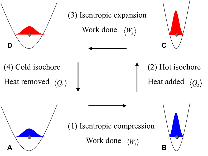
Figure 1: Quantum Otto cycle of a harmonic oscillator with time-dependent frequency. The thermodynamic cycle consists of two unitary (compression and expansion steps 1 and 3) and two isochoric processes (heating and cooling steps 2 and 3).

During the first and third strokes (compression and expansion), the quantum oscillator is isolated and only work is performed by changing the frequency in time. Since the dynamic is unitary, the Schrödinger equation for the parametric harmonic oscillator can be solved exactly for any given frequency modulation def08 ; def10 . The corresponding work values are given by aba12 ,

$$\left\langle W_{1}\right\rangle = \frac{\hbar}{2}(\omega_{2}Q^{\ast}_{1}-\omega_{1})\coth\left(\frac{\beta_{1}\hbar\omega_{1}}{2}\right),$$ (1)

$$\left\langle W_{3}\right\rangle = \frac{\hbar}{2}(\omega_{1}Q^{\ast}_{3}-\omega_{2})\coth\left(\frac{\beta_{2}\hbar\omega_{2}}{2}\right),$$ (2)

where we have introduced the dimensionless adiabaticity parameter $Q^{*}_{i}$ $(i=1,3)$ hus53 . It is defined as the ratio of the mean energy and the corresponding adiabatic mean energy and is thus equal to one for adiabatic processes def10 . Its explicit expression for any frequency modulation $\omega_{t}$ may be found in Refs. def08 ; def10 . On the other hand, the heat exchanged with the reservoirs during the thermalization step (the hot isochoric process) reads,

$$\left\langle Q_{2}\right\rangle=\frac{\hbar\omega_{2}}{2}\left[\coth\left(\frac{\beta_{2}\hbar\omega_{2}}{2}\right)-Q^{\ast}_{1}\coth\left(\frac{\beta_{1}\hbar\omega_{1}}{2}\right)\right].$$ (3)

For an engine, the produced work is negative, $\left\langle W_{1}\right\rangle+\left\langle W_{3}\right\rangle<0$, and the absorbed heat is positive, $\left\langle Q_{2}\right\rangle>0$.

The dynamics of the quantum Otto engine may be sped up with the help of STA techniques applied to the compression and expansion steps. The STA protocols suppress the unwanted nonadiabatic transitions and thereby reduce the associated entropy production fel00 ; rez06 ; aba12 ; aba16 . The effective Hamiltonian of the oscillator is then of the form,

$$H_{\mathrm{eff}}(t)=H_{0}(t)+H_{\text{STA}}^{i}(t),$$ (4)

where $H_{\text{STA}}^{i}(t)$ is the STA driving Hamiltonian and $i=(1,3)$ indicates the respective compression/expansion step. The STA protocol satisfies boundary conditions which ensure that initial and final expectation values $\langle H_{\text{STA}}^{i}(0,\tau)\rangle$ vanish:

$$\begin{array}[]{lcr}\omega(0)=\omega_{i},&\dot{\omega}(0)=0,&\ddot{\omega}(0)=0,\\ \omega(\tau)=\omega_{f},&\dot{\omega}(\tau)=0,&\ddot{\omega}(\tau)=0,\end{array}$$ (5)

where $\omega_{i,f}=\omega_{1,2}$ denote the respective initial and final frequencies of the compression/expansion steps. The conditions (5) are, for example, satisfied by iba12 ; cam13 ; def14 ,

$$\omega(t)=\omega_{i}+10(\omega_{f}-\omega_{i})s^{3}-15(\omega_{f}-\omega_{i})s^{4}+6(\omega_{f}-\omega_{i})s^{5},$$ (6)

where we have introduced $s=t/\tau$.

Efficiency and power are the two main quantities characterizing the performance of a heat engine. We define the efficiency of a STA engine as aba17 ,

$$\eta_{\text{STA}}=\frac{\mathrm{energy\,output}}{\mathrm{energy\,input}}=\frac{-(\left\langle W_{1}\right\rangle_{\text{STA}}+\left\langle W_{3}\right\rangle_{\text{STA}})}{\left\langle Q_{2}\right\rangle+\left\langle H^{1}_{\mathrm{STA}}\right\rangle_{\tau}+\left\langle H^{3}_{\mathrm{STA}}\right\rangle_{\tau}},$$ (7)

where $\left\langle H_{\text{STA}}^{i}\right\rangle_{\tau}=(1/\tau)\int_{0}^{\tau}dt\left\langle H_{\text{STA}}^{i}(t)\right\rangle$ is the time-average of the mean STA driving. Equation (7) takes the energetic cost of the STA driving along the compression/expansion steps into account. It reduces to the adiabatic efficiency $\eta_{\text{AD}}$ in the absence of these two contributions. For further reference, we additionally introduce the usual nonadiabatic efficiency of the engine, $\eta_{\text{NA}}=-(\left\langle W_{1}\right\rangle+\left\langle W_{3}\right\rangle)/\left\langle Q_{2}\right\rangle$, based on the formulas (2)-(4) in the absence of any STA protocol.

The power of the STA machine is on the other hand,

$$P_{\text{STA}}=-\frac{\left\langle W_{1}\right\rangle_{\text{STA}}+\left\langle W_{3}\right\rangle_{\text{STA}}}{\tau_{\text{cycle}}}.$$ (8)

Since the STA protocol ensures adiabatic work output, $\left\langle W_{i}\right\rangle_{\text{STA}}=\left\langle W_{i}\right\rangle_{\text{AD}}$ $(i=1,3)$, in a shorter cycle duration $\tau_{\text{cycle}}$, the superadiabatic power $P_{\text{STA}}$ is always greater than the nonadiabatic power $P_{\text{NA}}=-(\left\langle W_{1}\right\rangle+\left\langle W_{3}\right\rangle)/{\tau_{\text{cycle}}}$ aba17 . This ability to considerably enhance the power of a thermal machine is a key advantage of the STA approach. In the following, we explicitly evaluate the energetic cost of the STA driving, the efficiency (7) and the power (8) for the CD, LCD and IE methods.

III Counterdiabatic driving (CD)

We begin by analyzing the case of counterdiabatic driving (CD), which was first introduced by Demirplak and Rice dem03 and later independently developed by Berry ber09 . The method has recently been implemented experimentally in a trapped-ion system an16 . The goal of counterdiabatic driving (also called transitionless quantum driving) is to find a Hamiltonian $H_{\text{CD}}$ for which the adiabatic approximation to the original Hamiltonian $H_{0}$ is the exact solution of the time-dependent Schrödinger equation for $H_{\text{CD}}$. The explicit form of $H_{\text{CD}}$ is,

$$H_{\text{CD}}(t) = H_{0}(t)+i\hbar\sum_{n}(|\partial_{t}n\rangle\langle n|-\left\langle n|\partial_{t}n\right\rangle|n\rangle\langle n|)$$ (9)

$$= H_{0}(t)+H_{\text{STA}}^{\text{CD}}(t),$$

where $H_{\text{STA}}^{\text{CD}}$ is the STA driving Hamiltonian. For a time-dependent harmonic oscillator, it is given by mug10 ; tor13 ,

$$H_{\text{SA}}^{\text{CD}}(t)=-\frac{\dot{\omega_{t}}}{4\,\omega_{t}}({x}{p}+{p}{x}).$$ (10)

The Hamiltonian (9) is quadratic in ${x}$ and ${p}$, so it may be considered describing a generalized harmonic oscillator with a nonlocal operator ber85 ; mug10 ; che10 :

$$H_{\text{CD}}(t)=\frac{p^{2}}{2m}+\left(-\frac{\dot{\omega_{t}}}{4\omega_{t}}\right)(xp+px)+\frac{m\omega_{t}^{2}x^{2}}{2}.$$ (11)

Following Ref. mis17 , we may rewrite Eq. (11) as,

$$H_{\text{CD}}(t)=\hbar\Omega_{t}\left({b_{t}}^{\dagger}{b}_{t}+1/2\right)$$ (12)

with the instantaneous ladder operators ${b}_{t}$,

$${b}_{t}=\sqrt{\frac{m\Omega_{t}}{2\hbar}}\left(\zeta_{t}{x}+\frac{i{p}}{m\Omega_{t}}\right),$$ (13)

and the effective frequency,

$$\Omega_{t}=\omega_{t}\sqrt{1-\dot{\omega}_{t}^{2}/(4\omega_{t}^{4})},$$ (14)

with $\zeta_{t}=1+\dot{\omega}_{t}/(2i\omega_{t}\Omega_{t})$. Note that $\Omega_{t}^{2}>0$ to avoid trap inversion. This condition limits the rate of the frequency variation $\dot{\omega}_{t}$. Using the above equations, the adiabaticity parameter may be simply expressed as the ratio mis17 ,

$$Q^{\ast}_{\mathrm{CD}}(t)=\frac{\omega_{t}}{\Omega_{t}}.$$ (15)

The adiabaticity parameter $Q^{\ast}_{\mathrm{CD}}$ is plotted as a function of the time $t/\tau$ for the compression step in Fig. 2 (the corresponding result for the expansion is simply the mirror image). We observe that $Q^{\ast}_{\mathrm{CD}}$ approaches the adiabatic value one at the end of the driving, as it should, and it is much smaller than the nonadiabatic $Q^{\ast}_{\mathrm{NA}}$, as expected.

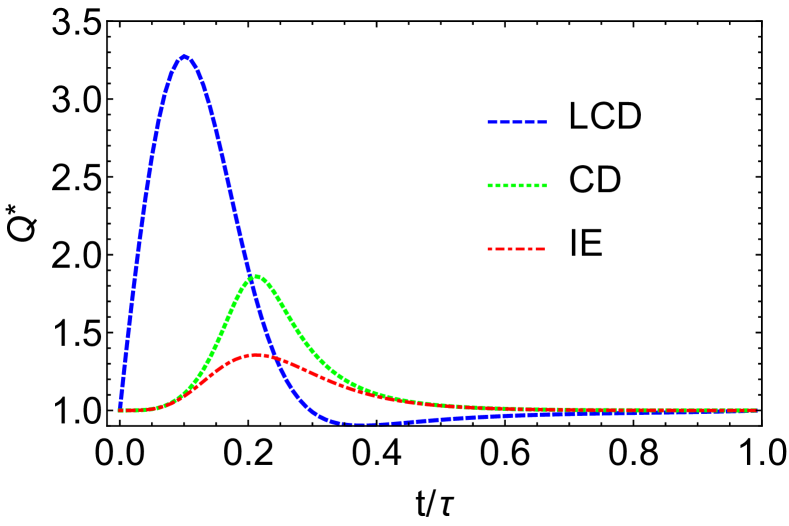
Figure 2: Adiabaticity parameter $Q^{*}$ for the compression step as a function of time for the three shortcut methods: counterdiabatic driving (CD) Eq. (15) (green dotted), local counterdiabatic driving (LCD) Eq. (21) (blue dashed) and inverse engineering (IE) Eq. (30) (red dotted-dashed) ($\omega_{1}/\omega_{2}=0.15$).

We proceed by evaluating the mean energy of the effective harmonic oscillator (12) at any time $t$, assuming that it is initially in a thermal state $P_{n}^{i}=\exp(-\beta_{i}E_{n}^{i})/Z_{i}$ at inverse temperature $\beta_{i}$. We obtain,

$$\langle H_{\mathrm{CD}}(t)\rangle = \sum_{n}\hbar\omega_{t}(\langle m\rangle_{n,t}+1/2)P_{n}^{i}$$ (16)

$$= \frac{\omega_{t}}{\omega_{i}}Q^{\ast}_{\mathrm{CD}}\langle H(0)\rangle,$$

where we have used the following expression for the mean quantum number, $\langle m\rangle_{n,t}+1/2=(n+1/2)Q^{\ast}_{\mathrm{CD}}$ def08 ; def10 , and $\langle H(0)\rangle=\hbar\omega_{i}\coth(\beta\hbar\omega_{i}/2)/2$. The expectation value of the CD driving finally follows as,

$$\langle H_{\mathrm{STA}}^{\mathrm{CD}}\rangle=\langle H_{\mathrm{CD}}(t)\rangle-\langle H_{0}(t)\rangle=\frac{\omega_{t}}{\omega_{i}}\langle H(0)\rangle\left(\frac{\omega_{t}}{\Omega_{t}}-1\right),$$ (17)

where we used $\langle H_{0}(t)\rangle=\langle H(0)\rangle\omega_{t}/\omega_{i}$ def10 . We numerically compute the energetic cost of the STA driving as the time average of Eq. (17). This time average is different from zero, although $\langle H_{\mathrm{STA}}(t=(0,t_{f}))\rangle=0$ in view of the boundary conditions (5). The corresponding efficiency (7) and power (8) are shown as a function of the driving time $\tau$ in Figs. 3 and 4 (green dotted).

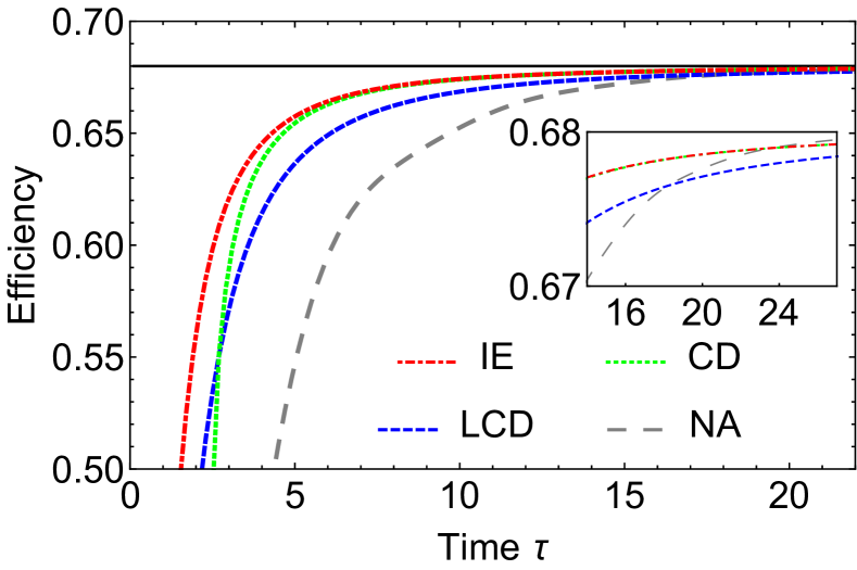
Figure 3: Efficiency as a function of the driving time $\tau$ for the three shortcut methods: counterdiabatic driving (CD) (green dotted), local counterdiabatic driving (LCD) (blue dashed) and inverse engineering (IE) (red dotted-dashed). The gray (large dashing) line shows the nonadiabatic efficiency (NA) without shortcut, while the black (solid) horizontal line is the adiabatic efficiency. Parameters are $\omega_{1}=0.32$, $\omega_{2}=1$, $\beta_{1}=0.5$ and $\beta_{2}=0.05$.

IV Local counterdiabatic driving (LCD)

A limitation of the CD method is that it requires the knowledge of the spectral properties of the original Hamiltonian $H_{0}(t)$ at all times to construct the auxiliary term $H_{\text{STA}}^{\text{CD}}(t)$ in Eq. (9). A possibility to circumvent this problem is offered by the local counterdiabatic (LCD) approach iba12 ; cam13 , which has been experimentally demonstrated in Refs. sch10 ; sch11 ; bas12 . Here the nonlocal operator (11) is mapped onto a unitarily equivalent Hamiltonian with a local potential by applying the canonical transformation, $U_{x}=\exp\left({im\dot{\omega}_{t}x^{2}}/{4\hbar\omega}\right)$, which cancels the cross terms $xp$ and $px$. This leads to a new local counterdiabatic (LCD) Hamiltonian of the form iba12 ; cam13 ,

$$H_{\mathrm{LCD}}(t) = U_{x}^{\dagger}(H_{\mathrm{CD}}(t)-i\hbar\dot{U}_{x}U_{x}^{\dagger})U_{x}$$ (18)

$$= \frac{p^{2}}{2m}+\frac{m\tilde{\Omega}_{t}^{2}x^{2}}{2},$$

with the modified time-dependent squared frequency,

$${\tilde{\Omega}}^{2}(t)=\omega_{t}^{2}-\frac{3\dot{\omega}_{t}^{2}}{4\omega_{t}^{2}}+\frac{\ddot{\omega}_{t}}{2\omega_{t}}.$$ (19)

The Hamiltonian (18) still drives the evolution along the adiabatic trajectory of the system of interest. By demanding that $H_{\mathrm{LCD}}(0,\tau)=H_{\mathrm{0}}(0,\tau)$, and imposing $\dot{\omega}(\tau)=\ddot{\omega}(\tau)=0$, the final state is equal for both dynamics, even in phase, and the final vibrational state populations coincide with those of a slow adiabatic process iba12 . The frequency $\tilde{\Omega}^{2}(t)$ approaches $\omega^{2}(t)$ for very slow expansion/compression cam13 . The LCD technique may be applied as long as $\tilde{\Omega}_{t}^{2}>0$. The expectation value of the local counterdiabatic Hamiltonian may be computed in analogy to the conterdiabatic driving and reads aba17 ,

$$\langle H_{\mathrm{LCD}}(t)\rangle = \frac{\omega_{t}}{\omega_{0}}\left(1-\frac{\dot{\omega}_{t}^{2}}{4\omega_{t}^{4}}+\frac{\ddot{\omega}_{t}}{4\omega_{t}^{3}}\right)\langle H(0)\rangle$$ (20)

$$= \frac{\omega_{t}}{\omega_{0}}Q_{\mathrm{LCD}}^{\ast}\langle H(0)\rangle,$$

with the adiabaticity parameter,

$$Q^{\ast}_{\text{LCD}}(t)=1-\frac{\dot{\omega}_{t}^{2}}{4\omega_{t}^{4}}+\frac{\ddot{\omega}_{t}}{4\omega_{t}^{3}}.$$ (21)

The variation of the adiabaticity parameter as a function of $t/\tau$ is shown in Fig. 2. The expectation value of the LCD driving is moreover evaluated as before aba17 ,

$$\langle H_{\mathrm{STA}}^{\mathrm{LCD}}(t)\rangle = \langle H_{\mathrm{LCD}}(t)\rangle-\langle H_{0}(t)\rangle$$ (22)

$$= \frac{\omega_{t}}{\omega_{0}}\langle H(0)\rangle\left[-\frac{\dot{\omega}_{t}^{2}}{4\omega_{t}^{4}}+\frac{\ddot{\omega}_{t}}{4\omega_{t}^{3}}\right].$$

The corresponding numerically computed efficiency (7) and power (8) are shown as a function of the driving time $\tau$ in Figs. 3 and 4 (blue dashed).

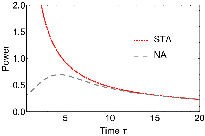
Figure 4: Power as a function of the driving time $\tau$ for the three shortcut methods: CD, LCD and IE lead to the same power (red dotted-dashed). The gray (large dashing) line shows the nonadiabatic (NA) efficiency. Same parameters as in Fig. 3

V Inverse engineering (IE)

An additional STA method is based on the design of appropriate parameter trajectories of the frequency by employing the Lewis-Riesenfeld invariants of motion lew69 supplemented by simple inverse-problem techniques pal98 . For the time-dependent harmonic oscillator described by $H_{0}(t)$, the state dynamics will be the solution of the corresponding Schrödinger equation based on the invariants of motion of the following form che10 ; che10a ,

$$I(t)=\frac{1}{2}\left(\frac{{x}^{2}}{\bar{b}^{2}}m\omega_{0}^{2}+\frac{1}{m}{\pi}^{2}\right),$$ (23)

where ${\pi}=\bar{b}{p}-m\dot{\bar{b}}{x}$ plays the role of a momentum conjugate to ${x}/\bar{b}$ and $\omega_{0}$ is in principle an arbitrary constant. The dimensionless scaling function $\bar{b}_{t}=\bar{b}(t)$ satisfies the Ermakov equation,

$$\ddot{\bar{b}}_{t}+\omega^{2}_{t}\bar{b}_{t}=\omega_{0}^{2}/\bar{b}_{t}^{3}.$$ (24)

Its solutions should be chosen real to make ${I}$ Hermitian. Whereas $\omega_{0}$ is often rescaled to unity by a scale transformation of $\bar{b}_{t}$, another convenient choice is $\omega_{0}=\omega(0)$. To achieve STA processes, $\omega(t)$ is first left undetermined and $\bar{b}_{t}$ is set to fulfil the equations ${I}(0)=H_{0}(0)$ and $[{I}(t_{f}),{H}_{0}(t_{f})]=0$. This guarantees that the eigenstates of ${I}$ and ${H}_{0}$ are the same at the initial and final times and can be done by satisfying the boundary conditions,

$$\begin{array}[]{lcr}\bar{b}(0)=1,&\dot{\bar{b}}(0)=0,&\ddot{\bar{b}}(0)=0,\\ \bar{b}(\tau)=\sqrt{\omega_{0}/\omega_{f}}=\gamma,&\dot{\bar{b}}(\tau)=0,&\ddot{\bar{b}}(\tau)=0,\end{array}$$ (25)

with $\omega_{0}=\omega(0)$ and $\omega_{f}=\omega(\tau)$. For an individual eigenstate $n$ of the oscillator Hamiltonian, the corresponding time-dependent instantaneous energy is,

$$\left\langle H_{\mathrm{IE}}(t)\right\rangle_{n}=\frac{\hbar(n+1/2)}{2\omega_{0}}\left(\dot{\bar{b}}_{t}^{2}+\omega^{2}_{t}\bar{b}_{t}^{2}+\frac{\omega_{0}^{2}}{\bar{b}^{2}_{t}}\right).$$ (26)

The parameter $\omega_{t}$ is here deduced from the Emarkov equation (24). To ensure the non-inversion of the trap, the condition $t_{f}>1/(2\omega_{f})$ should be satisfied. The expectation value of the STA at any given time follows as che10 ; che10a ,

$$\langle H_{\mathrm{IE}}(t)\rangle=\frac{\hbar}{2}\left[\frac{\dot{\bar{b}}_{t}^{2}}{2\omega_{0}}+\frac{\omega_{t}^{2}\bar{b}_{t}^{2}}{2\omega_{0}}+\frac{\omega_{0}}{2\bar{b}_{t}}\right]\coth\left(\frac{\beta\hbar\omega_{0}}{2}\right).$$ (27)

Using the relation $\bar{b}_{t}=(\omega_{0}/\omega_{t})^{1/2}$, we further have,

$$\dot{\bar{b}}_{t}=-\frac{1}{2}\left(\frac{\omega_{t}}{\omega_{0}}\right)^{1/2}\frac{\omega_{0}\dot{\omega}_{t}}{\omega_{t}^{2}}\hskip 14.22636pt\text{and}\hskip 14.22636pt\dot{\bar{b}}_{t}^{2}=\frac{1}{4}\frac{\omega_{0}\dot{\omega}_{t}^{2}}{\omega_{t}^{3}}.$$ (28)

Combining Eqs. (27) and (28), the time-dependent expectation value (27) can finally be written as,

$$\langle H_{\mathrm{IE}}(t)\rangle = \frac{\hbar}{2}\left[\frac{\dot{\omega}_{t}^{2}}{8\omega^{3}}+\frac{\omega_{t}}{2}+\frac{\omega_{t}}{2}\right]\coth\left(\frac{\beta\hbar\omega_{0}}{2}\right)$$ (29)

$$= \frac{\omega_{t}}{\omega_{0}}\langle H(0)\rangle\left[1+\frac{\dot{\omega}_{t}^{2}}{8\omega_{t}^{4}}\right].$$

The associated adiabaticity parameter hence reads,

$$Q_{\mathrm{IE}}^{\ast}(t)=1+\frac{\dot{\omega}_{t}^{2}}{8\omega_{t}^{4}},$$ (30)

as shown in Fig. 2 as a function of $t/\tau$. We may again deduce the expectation value of the IE driving as,

$$\langle H_{\mathrm{STA}}^{\mathrm{IE}}(t)\rangle=\langle H_{\mathrm{IE}}(t)\rangle-\langle H_{0}(t)\rangle=\frac{\omega_{t}}{\omega_{0}}\langle H(0)\rangle\frac{\dot{\omega}_{t}^{2}}{8\omega_{t}^{4}}.$$ (31)

The corresponding numerically computed efficiency (7) and power (8) are shown as a function of the driving time $\tau$ in Figs. 3 and 4 (red dotted-dashed).

Figure 5: Power-efficiency diagram for the three shortcut methods: counterdiabatic driving (CD) (green dotted), local counterdiabatic driving (LCD) (blue dashed) and inverse engineering (IE) (red dotted-dashed). The gray (large dashing) line shows the nonadiabatic efficiency (NA) without shortcut. Same parameters as in Fig. 3.

VI Discussion and conclusions

We have performed a detailed analysis of the performance of a STA quantum harmonic heat engine, using three commonly employed techniques: CD, LCD and IE. These three methods emulate adiabatic processes in finite time. We have first compared the time-dependent adiabaticity parameter $Q^{*}(t)$, Eqs. (15), (21) and (30), for all three STA approaches (shown in Fig. 2). We observe that while all three methods lead to $Q^{*}(\tau)=1$, per construction, the time dependence of $Q^{*}(t)$ may widely differ. The overall lowest value is achieved by inverse engineering (IE), which therefore appears to be the most effective technique to reduce unwanted nonadiabatic transitions.

We have further numerically calculated the energetic cost of the STA driving as the time average of the expectation value of the respective STA Hamiltonians, given in Eqs. (17), (22) and (31). The corresponding efficiencies and powers, that take into account this energetic cost, are presented in Figs. 3 and 4. We first note that all three methods lead to a significant increase of the efficiency at short cycle times, compared to the standard NA engine without shortcut. We observe furthermore that they all simultaneously yield a large enhancement of the power in the same regime. STA engines thus always outperform their traditional counterparts for short cycle durations. This is a remarkable feature of STA boosted quantum heat engines. They hence appear as energy efficient thermal machines that are able to produce more output from the same input at higher power. This property follows from the fact that STA protocols, on the one hand, speed up the dynamics (therefore increasing power), and on the other hand, also ensure that the final state is an adiabatic state instead of a highly excited state (thus reducing entropy production and consequently increasing efficiency).

Our study finally establishes that among the three considered STA methods, inverse engineering (IE) offers the largest increase of efficiency. This result confirms and directly follows from our previous observation that IE is the most effective method to suppress nonadiabatic transitions. At the same time, all three approaches yield the same enhanced power, since they produce the adiabatic work output in much less time. These findings are illustrated in the power-efficiency diagram shown in Fig. 5. The latter clearly demonstrates the advantage of STA heat engines operating in finite-time.

- (1) H.B. Callen, Thermodynamics and an Introduction to Thermostatistics, (Wiley, New York, 1985).
- (2) Y.A. Cengel and M.A. Boles, Thermodynamics. An Engineering Approach, (McGraw-Hill, New York, 2001).
- (3) B. Andresen, P. Salamon, and R. S. Berry, Thermodynamics in finite time, Phys. Today 37, 62 (1984).
- (4) B. Andresen, Angew. Chem. Int. Ed. 50, 2690 (2011).
- (5) N. Shiraishi, K. Saito, and H. Tasaki, Phys. Rev. Lett. 117, 190601 (2016).
- (6) T. Feldmann and R. Kosloff, Phys. Rev. E 61, 4774 (2000).
- (7) Y. Rezek and R. Kosloff, New. J. Phys. 8, 83 (2006).
- (8) O. Abah, J. Rossnagel, G. Jabob, S. Deffner, F. Schmidt-Kaler, K. Singer, and E. Lutz, Phys. Rev. Lett. 112, 030602 (2012).
- (9) O. Abah and E. Lutz, EPL 113, 60002 (2016).
- (10) American Physical Society Energy Efficiency Report (2008), http://www.aps.org/energyefficiencyreport
- (11) E. Torrontegui et al, Chapter 2. Shortcuts to adiabaticity, Adv. At. Mol. Opt. Phys. 62, 117 (2013).
- (12) S. Deffner, C. Jarzynski, and A. del Campo, Phys. Rev. X 4, 021013 (2014).
- (13) M. G. Bason, M. Viteau, N. Malossi, P. Huillery, E. Arimondo, D. Ciampini, R. Fazio, V. Giovannetti, R. Mannella, and O. Morsch, Nat. Phys. 8, 147 (2012).
- (14) R. Bowler, J. Gaebler, Y. Lin, T. Tan, D. Hanneke, J. Jost, J. Home, D. Leibfried, and D. Wineland, Phys. Rev. Lett. 109 080502 (2012).
- (15) A. Walther, F. Ziesel, T. Ruster, S. T. Dawkins, K. Ott, M. Hettrich, K. Singer, F. Schmidt-Kaler, and U. Poschinger, Phys. Rev. Lett. 109, 080501 (2012).
- (16) S. An, D. Lv, A. del Campo, and K. Kim, Nature Comm. 7, 12999 (2016).
- (17) J. Zhang, J. Hyun Shim, I. Niemeyer, T. Taniguchi, T. Teraji, H. Abe, S. Onoda, T. Yamamoto, T. Ohshima, J. Isoya, and D. Suter, Phys. Rev. Lett. 110, 240501 (2013).
- (18) Y-X. Du, Z-T. Liang, Y-C. Li, X-X. Yue, Q-X. Lv, W. Huang, X. Chen, H. Yan and S-L. Zhu, Nat. Comm. 7, 12479 (2016).
- (19) I. Martinez, A. Petrosyan, D. Guery-Odelin, E. Trizac, S. Ciliberto, Nature Phys. 12, 843 (2016).
- (20) M. Demirplak and S.A. Rice, J. Phys. Chem. A 107, 9937 (2003).
- (21) M. Demirplak and S. A. Rice, J. Chem. Phys. B, 109, 6838 (2005).
- (22) M.V. Berry, J. Phys. A: Math. Theor. 42, 365303 (2009)
- (23) S. Ibáñez, X. Chen, E. Torrontegui, J.G. Muga and A. Ruschhaupt, Phys. Rev. Lett. 109, 100403 (2012).
- (24) A. del Campo, Phys. Rev. Lett. 111, 100502 (2013).
- (25) X. Chen, A. Ruschhaupt, S. Schmidt, A. del Campo, D. Guéry-Odelin, and J.G. Muga, Phys. Rev. Lett. 104, 063002 (2010).
- (26) X. Chen, A. Ruschhaupt, S. Schmidt, S. Ibaáñez, and J.G. Muga, J. At. Mol. Sci. 1, 1 (2010).
- (27) X. Chen and J.G. Muga, Phys. Rev. A 82, 053403 (2010).
- (28) J. Deng, Q.-h. Wang, Z. Liu, P. Hänggi, and J. Gong, Phys. Rev. E 88, 062122 (2013).
- (29) Z. C. Tu, Phys. Rev. E 89, 052148 (2014).
- (30) A. del Campo, J. Goold, and M. Paternostro, Sci. Rep. 4, 6208 (2014).
- (31) M. Beau, J. Jaramillo, and A. del Campo, Entropy 18, 168 (2016).
- (32) J. Jaramillo, M. Beau, and A. del Campo, New. J. Phys. 18, 075019 (2016).
- (33) L. Chotorlishvili, M. Azimi, S. Stagraczynski, Z. Toklikishvili, M. Schüler, and J. Berakdar, Phys. Rev. E 94, 032116 (2016).
- (34) A. C. Santos, R. D. Silva, and M. S. Sarandy, Phys. Rev. A 93, 012311 (2016).
- (35) Y. Zheng, S. Campbell, G. De Chiara, and D. Poletti, Phys. Rev. A 94, 042132 (2016).
- (36) I. B. Coulamy, A. C. Santos, I. Hen, and M. S. Sarandy, Front. ICT 3, 19 (2016).
- (37) S. Campbell and S. Deffner, Phys. Rev. Lett. 118, 100601 (2017).
- (38) K. Funo, J.-N. Zhang, C. Chatou, K. Kim, M. Ueda and A. del Campo, Phys. Rev. Lett. 118, 100602 (2017).
- (39) E. Torrontegui, I. Lizuain, S. González-Resines, A. Tobalina, A. Ruschhaupt, R. Kosloff and J. Muga, arXiv:1704.06704 (2017).
- (40) O. Abah and E. Lutz, EPL 118, 40005 (2017).
- (41) R. Kosloff, J. Chem. Phys. 80, 1625 (1984).
- (42) E. Geva and R. Kosloff, J. Chem. Phys. 96, 3054 (1992).
- (43) B. Lin and J. Chen, Phys. Rev. E 67, 046105 (2003).
- (44) H. T. Quan, Y. Liu, C. P. Sun, and F. Nori, Phys. Rev. E 76, 031105 (2007).
- (45) R. Kosloff and Y. Rezek, Entropy 19, 136 (2017).
- (46) S. Deffner and E. Lutz, Phys. Rev. E 77, 021128 (2008).
- (47) S. Deffner, O. Abah, and E. Lutz, Chem. Phys. 375, 200 (2010).
- (48) K. Husimi, Prog. Theor. Phys. 9, 381 (1953).
- (49) J.G. Muga, X. Chen, S. Ibáñez, I. Lizuain, and A. Ruschhaupt, J. Phys. B. At. Mol. Opt. Phys. 43, 085509 (2010).
- (50) M.V. Berry, J. Phys. A: Math. Gen. 18, 15 (1985).
- (51) H. Mishima and Y. Izumida, Phys. Rev. E 96, 012133 (2017).
- (52) J.F. Schaff, X.L. Song, P. Vignolo, and G. Labeyrie, Phys. Rev. A 82 033430 (2010).
- (53) J.F. Schaff, X.L. Song, P. Capuzzi, P. Vignolo, G. Labeyrie, EPL 93, 23001 (2011).
- (54) H.R. Lewis and W.B. Riesenfeld, J. Math. Phys. 10, 1458 (1969).
- (55) J.P. Palao, J.G. Muga, and R. Sala, Phys. Rev. Lett. 80, 5469 (1998).