Initial Results from Fitting Resolved Modes using HMI Intensity Observations

Abstract

The HMI project recently started processing the continuum intensity images following global helioseismology procedures similar to those used to process the velocity images. The spatial decomposition of these images has produced time series of spherical harmonic coefficients for degrees up to $\ell=300$, using a different apodization than the one used for velocity observations. The first 360 days of observations were processed and made available. In this paper I present initial results from fitting these time series using my state of the art fitting methodology and compare the derived mode characteristics to those estimated using co-eval velocity observations.

1 Introduction

Recently, the Helioseismic and Magnetic Imager (HMI) project started processing the HMI continuum intensity images following procedures similar to those used to process the MDI and HMI velocity images. This generated time series of spherical harmonic coefficients suited for global helioseismology mode fitting.

The spatial decomposition of apodized intensity images was carried out for the first 360 days of the HMI science-quality data, producing time series of spherical harmonic coefficients for degrees up to $\ell=300$. Since the oscillatory signal in intensity is not attenuated by a line of sight projection, the intensity images were apodized differently from the velocity images. Moreover, since the global helioseismology data processing pipeline was developed using velocity images, the automatic detection of discontinuities in the intensity data has yet to be implemented and validated. For that reason the HMI project has not yet applied its gap filling to the resulting time series.

While solar p-mode oscillations were detected in intensity decades ago by Woodard (1984) with the ACRIM instrument on board SMM, the intensity images in most spatially resolved experiments are not routinely analyzed. Indeed, neither GONG, nor MDI or HMI pipelines process the intensity images.

Historically, solar oscillation data have been acquired and analyzed using intensity fluctuations for integrated observations (see Salabert et al., 2013, for example). For a few cases, intensity images have been reduced (Corbard et al., 2013) and in most cases a cross-spectral analysis was carried out on $m$-averaged spectra and without the inclusion of any spatial leakage information (Oliviero et al., 2001; Barban et al., 2004).

None of these studies led to a routine reduction and analysis of the intensity images, since the “noise” properties of the intensity data are quite different from the velocity data and fewer modes can be fitted. Nevertheless, fitting intensity data allows for an independent validation of the fitting methodology and further confirmation for the need to fit an asymmetric profile. Indeed, the GONG, MDI and HMI pipelines are still fitting symmetric profiles to mode peaks that are known to be asymmetric. Moreover the GONG pipeline simply ignores the leakage matrix, while the MDI and HMI pipeline includes the leakage matrix but continues to routinely fit symmetric profiles.

The MDI and HMI mode fitting procedure was retrofitted to include an asymmetry, but when using asymmetric profiles it fits fewer modes successfully and it produces a more inconsistent set of modes with fitted epoch. Finally, the mode asymmetry measured by the MDI and HMI fitting procedure barely changes with time or activity level, while the mode asymmetry measured by my methodology shows changes that correlate with the solar activity levels (see Korzennik, 2013).

By fitting the intensity and the velocity independently we can validate both the inclusion of the leakage matrix and the proper modeling of the asymmetry. Indeed, the intensity leakage is substantially different from the velocity leakage and the mode frequency ought to be the same whether the oscillatory signal is observed and measured in intensity or velocity. By contrast a cross-spectral analysis models both the intensity and the velocity spectra but fits a single parameter for the mode frequency, hence the velocity and intensity frequency is the same by construct.

In this paper I present my first attempt to fit these time series, using my state of the art fitting methodology (Korzennik, 2005, 2008). While that method is in principle perfectly suited to velocity or intensity observations, a leakage matrix specific to intensity observations was needed.

I fitted four consecutive 72-day long time series of intensity observations as well as one 288-day long time series (i.e., one four times longer). I carried out my mode fitting using the same procedures as I use for velocity observations, although I first refined the initial guess used for the mode profile asymmetry to be appropriate for intensity observations, and used a leakage matrix appropriate for intensity observations. I also ran my fitting procedure by forcing the mode profile to be symmetric. Finally, in order to extend the comparison to the 288-day long time series, I ran my fitting procedure on the same co-eval 288-day long time series using symmetric mode profiles and velocity observations.

I describe in Section 1.3 the various leakage matrix coefficient estimates I computed and/or used, and how I tried to validate them against the observed power distribution with $m$. The results from fitting intensity observations are presented in Section 2, and I first compare, in Section 2.4, the results obtained from fitting the same intensity observations time series using two different leakage matrices. Section 2.5 shows comparisons between mode parameters derived from fitting intensity and velocity observations, all using my fitting methods, but also cases run leaving the mode profile symmetric.

1.1 Data Set Used

The data set used for this study are time series of spherical harmonic coefficients computed by the HMI project at Stanford using the continuum intensity images taken by HMI on board the Solar Dynamic Observer (SDO). This data set is tagged at the SDO HMI and AIA Joint Science Operations Center (JSOC) as hmi.Ic_sht_72d. Four consecutive time series, each 72-day long, were produced for degrees up to $\ell=300$ and for all azimuthal orders, $m$, starting on 2010.04.30 at 00:00:00 TAI. These time series were not gap-filled, although the fill factors are high, namely between 97.078 and 99.660%. One 288-day long time series was constructed using, for consistency with previous analysis, four 72-day long time series starting on 2010.07.11 TAI (i.e., 72$\times$72 days after the start of the Michelson Doppler Imager, or MDI, science-quality data). The start and end time of the fitted time series and their respective duty cycles are listed in Table 1.

1.2 Brief Description of the Fitting Methodology

My state of the art fitting methodology is described at length in Korzennik (2005, 2008). The first step consists in computing sine multi-taper power spectra, with the number of tapers optimized to match the anticipated effective line-width of the modes being fitted, hence the number of tapers is not constant for a given time series length (see Korzennik, 2005, for details). The second step consists in fitting simultaneously all the azimuthal orders for a given mode, using a fraction of the power spectrum centered around the fitted mode. Each singlet, i.e.: ($n,\ell,m$), is modeled by an asymmetric mode profile characterized by its own frequency, amplitude and background, and by a line-width and asymmetry that is the same for all azimuthal orders, hence fitted model assumes that the FWHM and the asymmetry are independent of $m$ The fitted model includes a complete leakage matrix, where the leaked modes, modes for the same $n$ but a different $\ell$ and $m$, are attenuated by the ratio of the respective leakage matrix components. Contamination by nearby modes, namely modes with a different $n$, $\ell$ and $m$, is also included in the model when these modes are present in the spectral fitting window.

The model is fitted simultaneously, in the least-squares sense, to the observed $2\ell+1$ multi-tapered power spectra. For numerical stability the fitting is done in stages, i.e., not all the parameters are fitting simultaneously right away, and a sanity check is performed along the way: modes whose amplitude is not above some threshold based on the spectrum SNR are no longer fitted. A third step consists in iterating the fitting of each mode using the results of the previous iteration to account for the mode contamination.

Sections of power spectra, $P_{n,\ell,m}(\nu)$ are modeled as

$$P_{n,\ell,m}(\nu) = \Sigma_{\ell^{\prime},m^{\prime}}\left(\frac{C(\ell,m;\ell^{\prime},m^{\prime})}{C(\ell,m;\ell,m)}A_{n,\ell^{\prime},m^{\prime}}{\cal L}(\frac{\nu-\nu_{n,\ell^{\prime},m^{\prime}}}{2\,\Gamma_{n,\ell^{\prime}}},\alpha_{n,\ell^{\prime\prime}})+B_{n,\ell^{\prime},m^{\prime}}\right)$$ (2)

$$+\Sigma_{n^{\prime}}P_{n^{\prime},\ell,m}(\nu)$$

where $\nu$ is the frequency, ${\cal L}$ a generalized asymmetric Lorentzian, defined as

$${\cal L}(x,\alpha)=\frac{1+\alpha({x}-\frac{\alpha}{2})}{1+{x}^{2}}$$ (3)

and $\nu_{n,\ell,m},\Gamma_{n,\ell},\alpha_{n,\ell},A_{n,\ell,m}$, and $B_{n,\ell,m}$ are the mode frequency, FWHM, asymmetry, power amplitude, and background respectively, while $C(\ell,m;\ell^{\prime},m^{\prime})$ are the leakage matrix coefficients.

1.3 Intensity Leakage Matrix

1.3.1 Sensitivity Function and Limb Darkening

By contrast to the velocity oscillatory signal (see, for example, Korzennik, 2005), the intensity oscillatory signal is a scalar, leading to a simpler leakage matrix, namely:

$$C(\ell,m;\ell^{\prime},m^{\prime})=\int{\cal A}(\mu)J(\mu)\,Y_{\ell}^{m*}(\theta,\phi)\,Y_{\ell^{\prime}}^{m^{\prime}}(\theta,\phi)\,d\Omega$$ (4)

where $\theta$ is the co-latitude, $\phi$ the longitude, $\mu$ the fractional radius of the image of the solar disk, $\cal A$ the apodization used in the spatial decomposition, $J$ the sensitivity of the oscillatory signal, $Y_{\ell}^{m}$ the spherical harmonic of degree $\ell$ and azimuthal order $m$, and $d\Omega=\sin\theta d\theta d\phi$. The integral extends in $\theta$ and $\phi$ to cover the visible fraction of the Sun.

The sensitivity function, $J$, is likely to be equivalent to the limb darkening function, $I$, although this ought to be checked. In principle, the sensitivity function can be empirically computed from the observations by computing the RMS of the oscillatory signal as a function of position on the solar disk and reducing it to a function of $\mu$, the fractional radius. Hence, I computed the RMS of the residual intensity signal, after detrending the images, using HMI continuum images taken on ten consecutive days, for six different years. I detrended the images using a 15-minute long running mean, then computed, using the time series of residuals images, the mean and RMS around the mean of the residual signal, rebinned as a function of fractional radius, $\mu$, and normalized to unity at disk center. The solar limb darkening, for a set of wavelengths, has been measured and is reported in Pierce & Slaughter (1977).

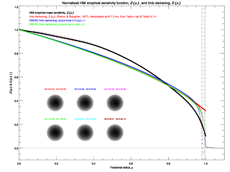
Figure 1: Empirical sensitivity functions, $J(\mu)$, and limb-darkening functions, $I(\mu)$, as a function of the fractional radius, $\mu$. The colored dash curves are estimates of $J(\mu)$ derived from 10 days of data taken in six consecutive years. The images of the RMS of the residuals used for this derivation are shown with the corresponding color-coded time ranges. The black solid line is the average of these six profiles, and the black dots the corresponding polynomial fit to this average that was used for one leakage matrix computation. The colored dots and circles correspond to limb-darkening profiles computed using different polynomial parametrization: Tables II and IV from Pierce & Slaughter (1977), interpolated for $\lambda=617.3$ nm, and coefficients used by the Stanford group (private communication). Open circles correspond to polynomials in $x=\ln(\mu)$, dots to polynomials in $\mu$. Note how the different limb-darkening representations disagree only near the limb, and that the polynomial parametrization with respect to $x=\ln(\mu)$ leads to negative values near the limb. Vertical lines are drawn to indicate the location of the limb and the edges of the cosine bell apodization used for the intensity observations.

The empirical sensitivity functions I derived for each year, the average for the six years, and the limb-darkening profiles given in Pierce & Slaughter (1977) interpolated at $\lambda=617.3$ nm, the wavelength HMI is observing at (Schou et al., 2012; Couvidat et al., 2012, 2016), and the profiles used by the Stanford group (private communication) are all compared in Fig. 1. One additional complication is the behavior near the limb of the different formulations of the polynomial representation of the limb-darkening, given either as a function of $x=\ln(\mu)$ or $\mu$; see Tables II or IV of Pierce & Slaughter (1977).

Since the intensity oscillatory signal is not attenuated by the line of sight projection, the apodization for the intensity images could be pushed closer to the edge of the solar disk without substantially adding noise, like in the case of velocity. The apodization was chosen by the Stanford group to start at $\mu=0.98$, consisting of a cosine bell attenuation that spans a range in $\mu$ of $0.015$, as indicated by the vertical lines drawn in Fig. 1.

The different profiles shown in Fig. 1 are somewhat similar. Note how the empirical sensitivity profiles resulting from processing each of the six years are nearly identical. They deviate from the limb-darkening profiles, suggesting an increased sensitivity for $0.3\leq\mu\leq 0.6$, and a sharper decrease in sensitivity for $\mu\geq 0.8$. In contrast, the different limb darkening profiles are almost identical for $\mu<0.9$, except that the polynomial parametrization in $x=\ln(\mu)$ leads to negative values close to the limb, including the one based on the Stanford version 2 coefficients. The polynomial parametrization in $\mu$ of the limb-darkening does not include the progressive attenuation near the limb resulting from an empirical determination of the sensitivity profile, although the contribution to the leakage matrix of the regions with $\mu\geq 0.98$ is dominated by the apodization.

The precise profile to be used for the computation of the intensity leakage matrix is yet to be determined. I opted to use a polynomial parametrization in $\mu$, and either the limb-darkening, $I(\mu)$, given by the coefficients in Table IV of Pierce & Slaughter (1977), interpolated at $\lambda=617.3$ nm, or a polynomial in $\mu$ fitted to my determination of the averaged empirical sensitivity function, $\bar{J}(\mu)$, for all six processed years. I also used the leakage matrix computed by the HMI group at Stanford (Larsen, private communication).

1.3.2 Computation and Validation of the Leakage Matrix

A leakage matrix is “simply” computed by generating images representing the quantity $J(\mu)\,Y_{\ell}^{m*}(\theta,\phi)$, or $I(\mu)Y_{\ell}^{m}(\theta,\phi)$ and processing them using the same spatial decomposition used for the observations.

The effects of the actual orientation, i.e., $P_{\rm eff}$, the effective position angle and $B_{o}$, the latitude at disk center, $D^{o}_{\odot}$, the finite observer to Sun distance, and the image pixelization, while not described explicitly here, are taken into account when computing the images that are decomposed to generate a leakage matrix (see Korzennik et al., 2004; Schou, 1999) . My computation evaluated $C_{\ell,m}(\delta\ell,\delta m)=C(\ell,m;\ell^{\prime},m^{\prime})$ for $\delta\ell=\pm 20$ and $\delta m=\pm 20$, while the HMI group at Stanford limited their evaluation to $\delta\ell=\pm 6$ and $\delta m=\pm 15$, where $\delta\ell=\ell^{\prime}-\ell$ and $\delta m=m^{\prime}-m$.

In an attempt to validate the different computations of leakage matrices suited for intensity observations, I choose to compare the variation with respect to $m$ (or the ratio ${m}/{\ell}$) of the leakage to the variation of the observed power.

We can assume that the mode amplitude ought to be uniform with $m$, in the absence of any physical mechanism that would modulate the amplitude with $m$. If this is indeed the case, the variation of the observed total power, or the measured power amplitude of the modes, is only the result of the variation of the leakage matrix with $m$. Therefore the total power variation with $m$ at a fixed $\ell$ should be proportional to the sum of sensitivity of the target mode plus the contribution of the leaks. We can thus equate the normalized total power

$$\bar{P}_{\ell,m}^{\rm Tot}=\frac{1}{P_{N}}=\Sigma_{\nu}\,P_{\ell,m}(\nu)$$ (5)

to

$$\bar{Q}_{\ell,m}^{\rm Tot}=\frac{1}{Q_{N}}\Sigma_{\delta\ell,\delta m}\,C^{2}_{\ell,m}(\delta\ell,\delta m)$$ (6)

where $P_{N}$ and $Q_{N}$ are normalization factors chosen to set $\bar{Q}_{\ell,m=0}^{\rm Tot}=\bar{P}_{\ell,m=0}^{\rm Tot}=1$.

On the other hand, the modes observed power amplitude, $A_{n,\ell,m}$, as measured by fitting the modes, should be proportional to the values of the $\delta\ell=\delta m=0$ leak, or $C^{2}_{\ell,m}(0,0)$. Hence the quantity

$$\bar{A}_{\ell,m}=\frac{1}{A_{N}}\Sigma_{n}\,A_{n,\ell,m}$$ (7)

is equal to the ratio

$$\bar{Q}_{\ell,m}=\frac{C^{2}_{\ell,m}(0,0)}{C^{2}_{\ell,m=0}(0,0)}$$ (8)

if $A_{N}$ is such that $\bar{A}_{\ell,m=0}=1$, since $\bar{Q}_{\ell,m=0}=1$ by construction.

In order to build statistical significance for the observed quantities $\bar{P}^{\rm Tot}_{\ell,m}$ and $\bar{A}_{\ell,m}$, I performed additional averaging over a range in $\ell$ ($\delta\ell=\pm 1$), plus some smoothing over $m$ and symmetrization in $m$.

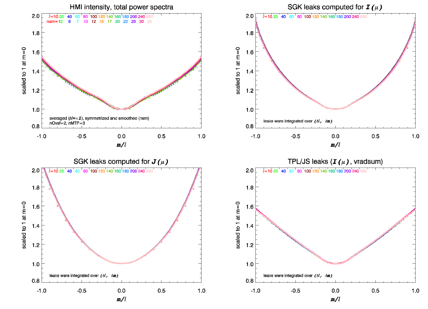
Figure 2: Upper left panel: total power in the power spectra of the HMI intensity oscillation signal, for a set of degrees, $\ell=10,20,(20),200,(40),280$, plotted as a function of the ratio $m/\ell$, and normalized to unity at $m=0$. The total power was smoothed in $m$ (as indicated by the $nsm$ key) and symmetrized with respect to $m/\ell$, and estimated using a $\delta\ell=\pm 1$ range in $\ell$ to increase the significance of the derived profiles. The other three panels show the sum of the leaks, for the same set of degrees, also plotted as a function of the ratio $m/\ell$, and normalized to unity at $m=0$, i.e.,$\bar{Q}_{\ell,m}^{\rm Tot}=\frac{1}{Q_{N}}\Sigma_{\delta\ell,\delta m}\,C^{2}_{\ell,m}(\delta\ell,\delta m)$. Each of these three panels corresponds to leakage estimates based on different $J(\mu)$ or $I(\mu)$ profiles.

Figures 2 to 4 show these comparisons, using three distinct leakage matrices and a set of degrees. While the overall variation with $m/\ell$ agrees qualitatively, none of the leakage matrices lead to $\bar{Q}^{\rm Tot}_{\ell,m}$ or $\bar{Q}_{\ell,m}$ profiles that closely match the observed quantities, $\bar{P}^{\rm Tot}_{\ell,m}$ or $\bar{A}_{\ell,m}$ respectively. Moreover, the two methods do not agree as to which case models best the observed quantities. This apparent contradiction could be the result of the wrong assumption that the mode power is independent of $m$. Since it is the solar rotation that breaks the spherical symmetry and thus “defines” $m$, it is not inconceivable that, while the solar rotation is slow compared to the oscillations, the rotation attenuates some azimuthal orders over others and produces an intrinsic variation of the modes amplitude with azimuthal order, $m$.

1.4 Seed Asymmetry for Intensity

Using high degree resolved modes, Duvall et al. (1993) were the first to notice that not only are the profiles of the modes asymmetric, but the asymmetry for velocity observations is of the opposite sign than the asymmetry for intensity observations. This asymmetry is, of course, also present at low and intermediate degrees, and is expected to be of opposite sign for velocity and intensity.

For each mode set, the fitting starts from some initial guess, also known as a seed. The seed file holds the list of modes to attempt to fit, i.e., the coverage in $(n,\ell)$, and for each mode a rather good initial guess of the mode’s central frequency, or multiplet, the frequency splitting parametrized by a polynomial expansion in $m$, its line-width and its asymmetry. The initial guesses for the asymmetry are set to be a smooth function of frequency, and for velocity observations, using my parametrization, are mostly negative. Since the asymmetry of the intensity observations is of the opposite sign, a new seed asymmetry had to be computed.

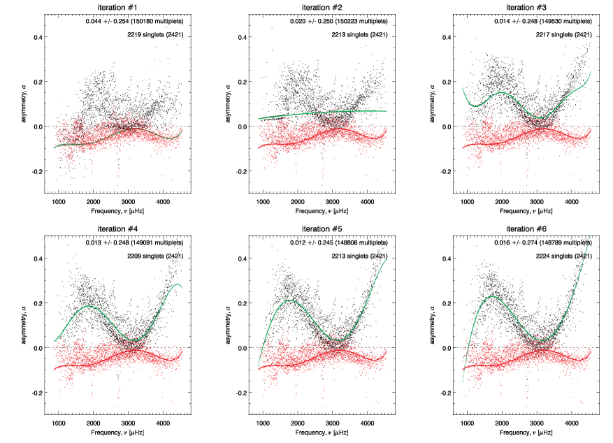
Figure 5: Values of the seed. i.e., initial guess, and fitted asymmetry, plotted as a function of frequency, for each iteration used in the refinement of the seed asymmetry values. The red dots are values of $\alpha^{V}_{n,\ell}$ resulting from fitting velocity observations, the black dots are values of $\alpha^{I}_{n,\ell}$ resulting from fitting intensity observations at each successive iteration. The red curves show the seed asymmetry $\alpha_{n,\ell}^{sV}$ used for velocity, the green curves show the seed asymmetry $\alpha_{n,\ell}^{sI}$ for intensity at each iteration. The mean and standard deviation of the changes in the fitted frequency values at each iteration are indicated in each panel. Note how even with initial negative values for the asymmetry, the resulting fitted asymmetries become mostly positive at the first iteration (upper left panel).

To accomplish this, I ran my second step, or initial fit, as described earlier in Section 1.2, using one 72-day long segment, and using at first the negative initial guesses for $\alpha$ appropriate for velocity observations, i.e., $\alpha_{n,\ell}^{sV}$. The resulting fitted asymmetries were mostly positives. I proceeded to fit a polynomial in $\nu$ to them and produced an updated seed file with new initial guesses for intensity observations, i.e., $\alpha_{n,\ell}^{sI}$. I repeated this procedure six times, as illustrated in Fig. 5, until the resulting mean change in the resulting fitted frequencies was negligible. The final parametrization of the initial guess for $\alpha_{n,\ell}^{sI}$ was subsequently used to fit all the intensity observations.

2 Fitting Results

For reasons of convenience explained earlier, the times series of spherical harmonic coefficients computed by spatially decomposing HMI continuum intensity images have not been gap filled. I computed sine multi-tapered power spectra for four consecutive 72-day long time series and one 288-day long time series. The power spectra were fitted using my fitting methodology, using the seed file adjusted to take into account the mode profile asymmetry for intensity observations, and two sets of leakage matrices: one computed by myself based on the limb-darkening parametrized by a 5 coefficient polynomial in $\mu$ (Pierce & Slaughter, 1977, interpolated at $\lambda=617.3$ nm) and one provided by the HMI group at Stanford, courtesy of Drs. Larson and Schou (private communication).

Only the 72-day long time series were fitted using both leakage matrices, and using an asymmetric profile. All the other cases were fitted using only the leakage matrix I computed, based on a limb-darkening profile. In order to assess the effect of fitting the asymmetry, I also fitted the intensity data with a symmetric profile. This was accomplished by modifying the seed file to set the asymmetry to zero, and changing the steps used in the fitting procedure to leave the asymmetry parameter null by never including it in the list of parameters to fit.

2.1 Intensity SNR Limitation

A major difference between velocity and intensity oscillatory signals, besides the sign of the asymmetry, is the nature of the so-called background noise, so called because it is a signal of solar origin that adds a noisy background level to the oscillatory signal. Intensity observations, whether disk integrated or resolved, show a noise contribution that increases as the frequency decreases, of a $\nu^{-1}$ nature. The detrending that was adequate for the velocity signal is no longer optimal for intensity, hence I modified the detrending I perform on the time series before computing the sine multi-taper power spectrum, from subtracting a 20-minute long running mean to subtracting an 11-minute long running mean. This filters out power below 1.52 $\mu$Hz rather than below 0.83 $\mu$Hz.

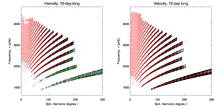
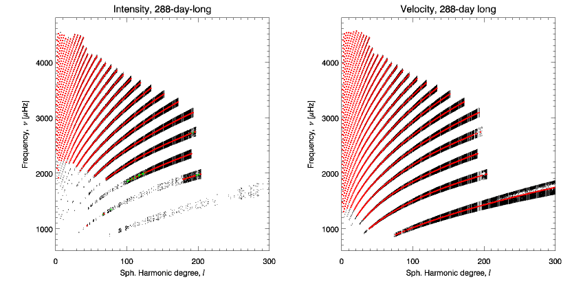
Figure 6: Coverage in the $\ell-\nu$ plane of the fitted modes. Black dots show singlets, red dots multiplets and green dot multiplets resulting from a less restrictive rule for the conversion of singlets to multiplets (see explanation in the text). The top two panels correspond to fitting one 72-day long time series, the bottom two panels to fitting one 288-day long time series. Panels on the left correspond to intensity observations, panels on the right to co-eval velocity observations. Note the reduced success rate in fitting intensity observations, especially for the low-order, low-frequency modes. Note also, the counter-intuitive higher success rate for fitting f-mode singlets for the 72-day long time series than for the 288-day long one, when using intensity observations.

Since my fitting methodology performs a sanity check at regular intervals, modes at low frequencies, where the background level is high for intensity observations, are no longer fitted. This attrition at low frequencies is illustrated in Fig. 6, where the $(n,\ell,m)$ singlets that were successfully fitted are shown in a $\ell-\nu$ diagram, and compared to the same representation when fitting a similar data set derived from gap-filled velocity observations.

Because the coverage in the $\ell-\nu$ space is a lot more sparse for intensity, I revised the procedure I use to derive multiplets, i.e., $(n,\ell)$, from singlets. That procedure fits a Legendre polynomial to all the successfully fitted frequencies, $\nu_{n,\ell,m}$, for a given $(n,\ell)$ mode as a function $m$ to derive a mode frequency, $\nu_{n,\ell}$, and frequency splitting coefficients. The procedure fits from one to 9 coefficients, performs a 3-sigma rejection of outliers, and computes a mode multiplet if and only if at least 1/8th of all the expected $m$ are used in the polynomial. This criteria worked fine when fitting velocity observations, but it eliminates most of the low-order, low-frequency modes, including all the $f$-modes when fitting intensity observations.

I re-adjusted this procedure to derive a second set of multiplets using a less stringent constraint, namely that at least only 1/16th of all the $m$ could be fitted. This led to some outliers that were then cleaned out by eliminating modes whose frequency do not fall on a smooth function of $\ell$ for each order, $n$. This is illustrated in Fig. 6 by the green dots.

2.2 Effect of Gap Filling and Longer Time Series on Low Frequency Noise

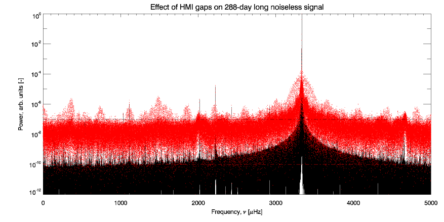
Figure 7: Effect of gaps on a noiseless data set. The black curve is the power spectrum of a simple sine wave, sampled every 45 seconds for 288 days. The red curve is that same sine wave but with values set to zero at times when HMI observations are missing for the 288-day long time series analyzed. The introduction of gaps scatters power and raises the background levels considerably, but uniformly with respect to frequency, compared to the gap-less noiseless case.

Since the time series of intensity spherical harmonic coefficients were not gap filled, I checked the contribution of the gaps to the background noise. A naive estimate, illustrated in Fig. 7, suggests that gaps scatter a lot of power into a higher background noise, including at low frequencies. I therefore adapted the gap filler I use for the GONG observations to gap fill one 72 day long time series of HMI intensity data. This gap filler is the same as the one used by the Stanford group to gap fill the MDI and HMI velocity data.

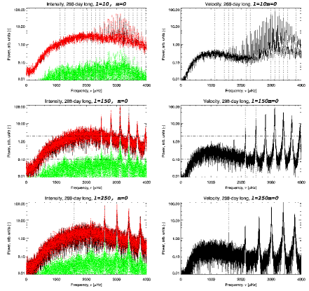
Figure 8: Examples of sine multi-taper zonal ($m=0$) power spectra computed using 72-day long (six leftmost panels) or 288-day long (six rightmost panels) time series. The panels in the first and third columns show power spectra of intensity observations derived from raw or gap-filled time series (red and black curves respectfully). The green curves are the difference between the spectra computed using raw or gap-filled time series. The second and forth columns show power spectra of gap-filled co-eval velocity observations. The vertical lines indicate the location of the modes being fitted. Each row corresponds to a different value of $\ell$ ($\ell=10,150,250$, top to bottom respectfully), the horizontal lines are drawn as fiducial lines to mark the background level around 2 mHz.

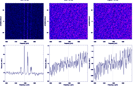
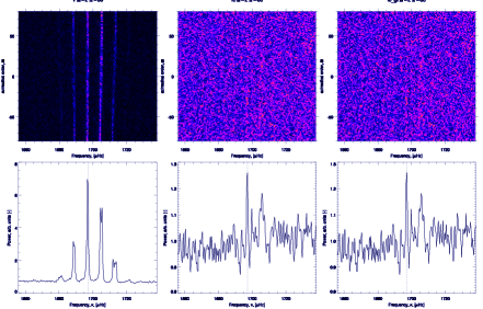
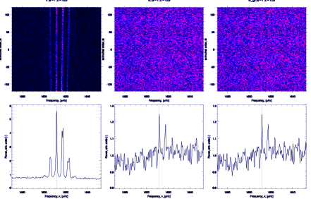
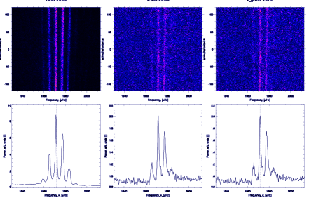
Figure 9: Stacked sections of power spectra, shown as a function of $\nu$ and $m$, and the corresponding $m$-averaged spectra, centered around a set of four modes for $(n,\ell)=(1,80),(2,80),(1,120)$ and $(2,120)$, computed using a 72-day long time series. The vertical lines indicate the mode frequency. Each set of six panels shows in the top row the stacked spectra, in the bottom row the corresponding $m$-averaged spectrum, and from left to right, spectra computed from the gap-filled velocity, the raw (i.e., with gaps) intensity and the gap-filled intensity co-eval time series. Stacked sections of power spectra are sections of spectra centered on the mode singlet frequency, $\nu_{n,\ell,m}$, computed using a very good estimate of the mode frequency and frequency splitting to offset in frequency the spectrum for each $m$ so as to co-align the target modes.

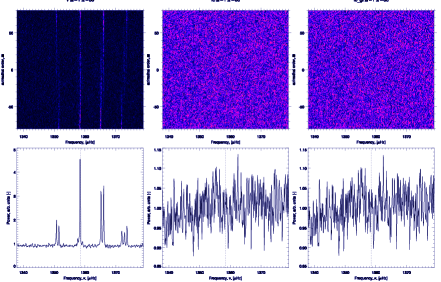
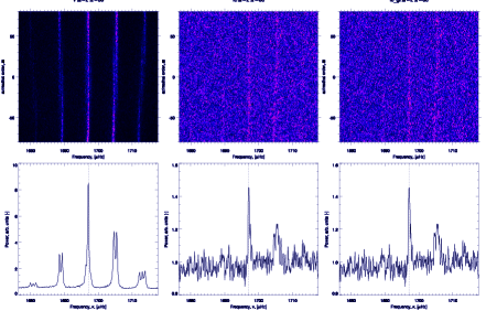
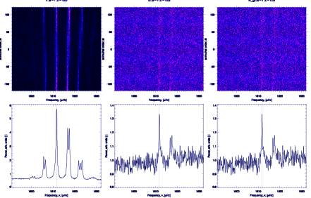
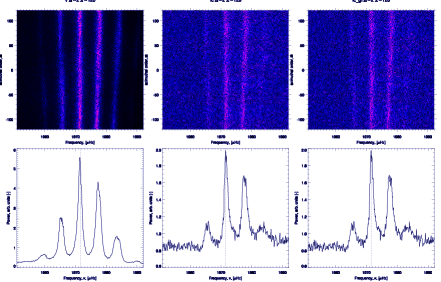
Figure 10: Stacked and $m$-averaged spectra, like in Fig. 9, but when using a 288-day long time series. The $(n,\ell)=(2,80)$ and $(1,120)$ modes become barely visible in intensity when using a longer time series.

Figures 8, 9 and 10 show that both gap filling and using longer time series do not reduce the low frequency background noise. Fig. 8 shows that (i) gap filling the intensity observations barely changes the background levels; (ii) the background level for intensity is about 20 times higher around 2 mHz than for velocity; and (iii) the longer time series do not lower the background but reduce the background realization noise. For the intensity observations, that reduction is not sufficient to see the low-order, low-frequency modes. Note also the clearly visible change of sign of the mode profiles asymmetry between intensity and velocity power spectra.

Figures 9 and 10 show (i) how the realization noise produces spikes that without proper “sanity check” can be easily confused as low amplitude modes, and (ii) that some modes peak above the noise in an $m$-averaged spectrum but can’t be discriminated from the noise when fitting singlets.

From these figures, one concludes that the power at low frequency is of solar origin and masks the oscillatory signal. The power scatter by the gaps at these frequencies is negligible, while increasing the length of the time series decreases the realization noise, but not the background level. Eventually, a very long time series may bring the realization noise to a level low enough to see a weak oscillatory signal emerge clearly above the background, but quadrupling the length is not enough. In fact, and somewhat counter-intuitively, quadrupling the length of the time series resulted in making fitting low frequency modes more difficult.

For completeness, I also fitted the 288-day long time series using gap-filled time series. As anticipated, the resulting number of fitted modes and their characteristics are barely different from the raw data: a few more singlets were fitted but the same number of multiplets were derived when the observations are gap filled. The mean of the difference between raw and gap-filled data in the derived frequencies is less than 1 nHz, with a standard deviation of 13 nHz and differences in the derived FWHM and asymmetry are negligible.

2.3 Results from 72-day and 288-day long Fitting

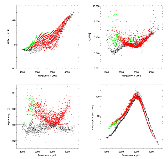
Figure 11: Mode characteristics derived from fitting a 72-day long time series, after converting singlets to multiplets. The panels show, as a function of frequency, the modes FWHM, $\Gamma$, frequency uncertainty, $\sigma_{\nu}$, asymmetry, $\alpha$, and, the mean mode amplitude, $\bar{A}_{n,\ell}=\frac{1}{N_{m}}\Sigma_{m}A_{n,\ell,m}$. The red and green circles correspond to fitting intensity observations, with the green circles resulting from a less restrictive constraint in the conversion of singlets to multiplets (see text and Fig. 6), the black dots corresponding to results from fitting co-eval velocity time series. Except for the low-order low-frequency modes, the FWHM and the frequency uncertainties derived using either velocity or intensity agree quite well. The asymmetry when fitting intensity observations is both of opposite sign to the asymmetry for velocity but also larger in magnitude. The mode power amplitude distribution, while peaking at the same frequency and being overall similar, shows a distinctive different distribution with frequency when fitting intensity rather than velocity observations. The green circles, resulting from estimating the multiplets using relaxed rules, appear to be consistent with their corresponding values derived from velocity but show a larger uncertainty. This in itself is not surprising since they are derived from fewer individually fitted singlets.

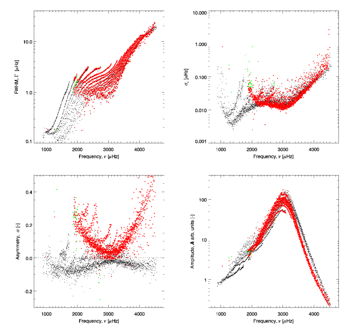
Figure 12: Mode characteristics derived from fitting a 288-day long time series, after converting singlets to multiplets, using the same representation as the one used in Fig. 11. Again, like for the 72-day long results, the frequency uncertainties derived using either velocity or intensity observations agree quite well. The asymmetry for intensity observations is both of opposite sign to the asymmetry for velocity observation and larger in magnitude. The mode power amplitude distributions derived from intensity or velocity observations also peak at the same frequency but are also more similar than for the 72-day long case. The frequency uncertainties are, as expected, reduced by a factor $\sqrt{{288}/{72}}=2$ when compared to values obtained using a shorter time series. By contrast to the 72-day long results, very few individual singlets were fitted for modes with $\nu<1800$ $\mu$Hz and $\Gamma<0.8$ $\mu$Hz.

Figures 11 and 12 show mode characteristics resulting from fitting 72-day and 288-day long time series, after converting singlets to multiplets. Table 2 lists the number of fitted modes (singlets) and the number of derived multiplets for each fitted time series, the different type of data and leakage matrix used. The FWHM, $\Gamma_{n,\ell}$, asymmetry, $\alpha_{n,\ell}$, the uncertainty of the fitted frequencies, $\sigma_{\nu_{n,\ell}}$ and the mode power amplitudes, $\bar{A}_{n,\ell}$, are plotted for the resulting multiplets, for one representative 72-day long set and for the 288-day long set. The corresponding values derived from fitting co-eval velocity observations are shown as well.

Except for the low-order low-frequency modes, the FWHM and the frequency uncertainties derived using either velocity or intensity observations agree quite well. As expected, the asymmetry derived from intensity observations is of opposite sign of the asymmetry derived from velocity observations but it is also larger in magnitude by about a factor two. The mode power amplitude variation with frequency is overall similar, whether measured using intensity or velocity observations, as it peaks at the same frequency but shows a somewhat different distribution. This is most marked for results from fitting 72-day long time series and at low frequencies. Most of the extra low-frequency modes derived from the 72-day long time series, using a less stringent constraint to derive multiplets, show consistent values that mostly agree with their velocity counterparts, except for higher uncertainties and larger FWHM at the lowest frequencies. The higher uncertainty in itself is not surprising since these multiplets are derived from fewer singlets, but the increase in FWHM cannot easily be explained.

Contrasting results from fitting 72-day long time series to those resulting from fitting 288-day long ones leads to the following observations: the mode FWHM, frequency uncertainty, asymmetry and power amplitude distribution are comparable, although (1) very few low frequency modes are successfully derived; (2) the frequency uncertainty is reduced as expected by about a factor 2, namely the square root of the ratio of the time series lengths; and (3) the scatter in the measured asymmetry is reduced for intensity as it is for velocity.

I have yet to fully understand why, when using the longer time series, almost no modes below $\nu<1800$ $\mu$Hz or $\Gamma<0.8$ $\mu$Hz could be fitted (see Fig. 6). This may suggest that despite appearing consistent, the low frequency modes derived using a shorter time series are suspicious and the methodology, especially the sanity check, needs to be adapted to the specifics of the noise distribution of the intensity signal.

2.4 Comparison using Different Leakage Matrices

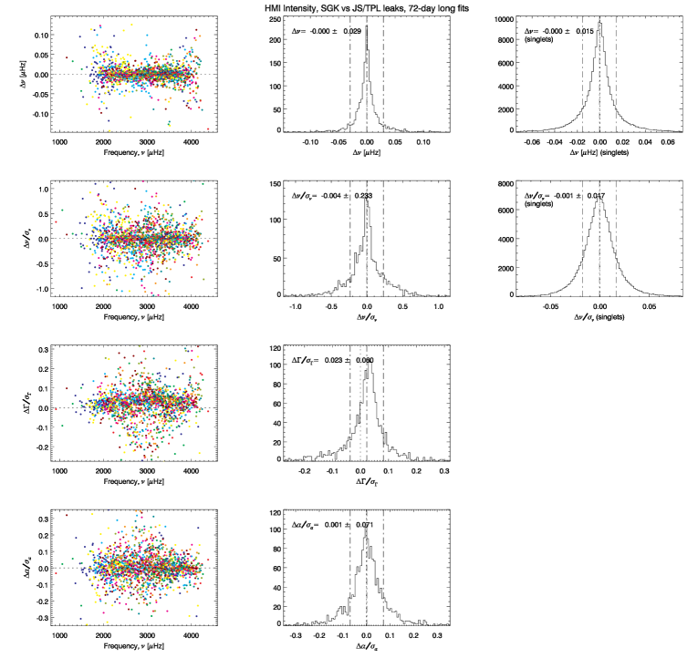
Figure 13: Comparison of mode characteristics derived from fitting a 72-day long time series, after converting singlets to multiplets, and for singlets, using two different leakage matrix computations, namely mine based on $I(\mu)$ and the one computed by the Stanford group. The panels show, top to bottom, raw and scaled frequency differences for multiplets and singlets, and FWHM and asymmetry scaled differences. The panels in the leftmost column show the multiplets’ differences with colors corresponding to the modes’ order, $n$. The panels in the middle column show the histogram distribution of the differences for the multiplets, while the panels in the rightmost column show the histogram distribution of the differences computed using singlets. Vertical lines are drawn at zero and at the mean plus or minus one standard deviation around the mean. Despite significant differences between the two leakage matrix coefficients (see, for example, Fig.4), the resulting parameters show little differences, both in term of bias and spread. Only the FWHM differences show a non-negligible bias.

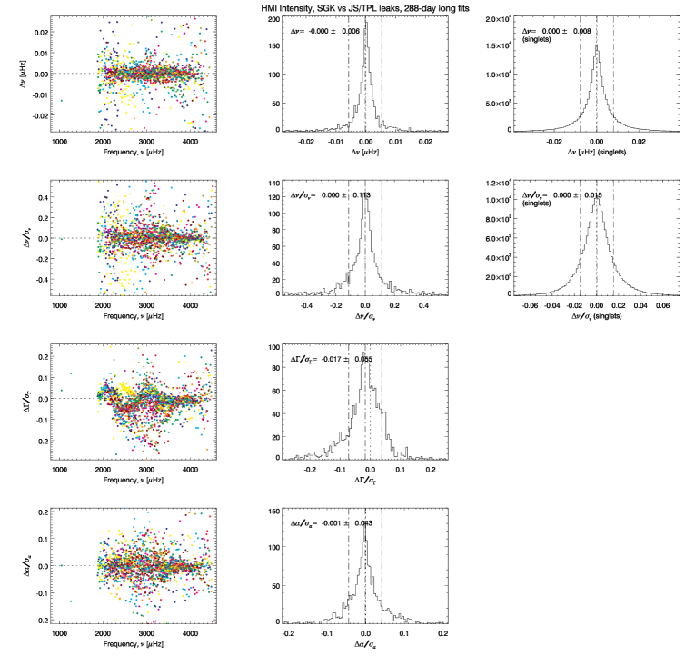
Figure 14: Comparison of mode characteristics derived from fitting a 288-day long time series, as shown in Fig. 13 for the 72-day long case, and using the same two different leakage matrix computations. The resulting bias and spread remain small. Again, the FWHM differences show a non-negligible bias, that while small, show a hint of systematic distribution with order and frequency.

Figures 13 and 14 shows a comparison of the mode parameters inferred by fitting the same time series of intensity observations, using the exact same methodology but two different estimates of the leakage matrix. Despite the different signature of the leakage sensitivity with $m$, the resulting fitted frequencies, and most of the other modes parameters, are barely different and show no systematic trends. Comparisons of the singlets frequency, or the singlets scaled frequency show a normal distribution with no significant bias and a very low scatter. Only the mode line-width, $\Gamma$, when fitting the longer time series, is systematically different, although not significantly. Of course, we cannot rule out that fitting much longer time series may lead to small but significant or systematic differences. Still, this comparison shows that for 72 and for 288-day long time series, the use of different leakage matrix estimates does not really affect the fitted values.

2.5 Comparison with Results from Fitting Velocity

Now that we have, for the first time, mode parameters resulting from fitting the same interval based on either velocity or intensity HMI observations, let us compare in detail the resulting mode characteristics. Despite the fact that the velocity time series were gap filled, while the intensity ones were not, we have shown that we can rule out that this affected the results and thus this comparison, because (i) the fill factors are already high; and (ii) the background signal at low frequency is any way much higher for intensity than for velocity.

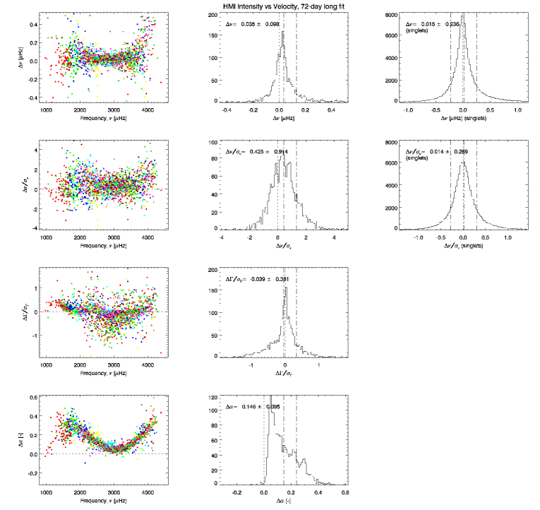
Figure 15: Comparison of mode characteristics derived from fitting a 72-day long time series, as shown in Fig. 13, but resulting from fitting co-eval intensity and velocity time series. The means and standard deviation of the differences are negligible for frequencies, $\nu$, and FWHM, $\Gamma$. As expected the differences in asymmetries are large and show a clear and smooth dependence on frequency.

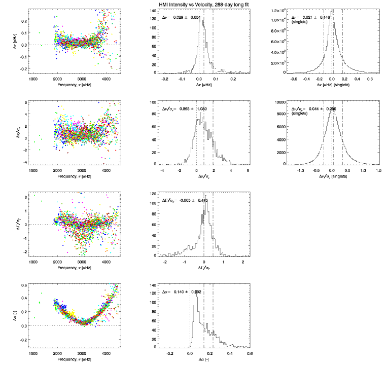
Figure 16: Comparison of mode characteristics derived from fitting a 288-day long time series, as shown in Fig. 15 for the 72-day long case, and also resulting from fitting co-eval intensity and velocity time series. Similarly to the 72-day long case, the differences in asymmetries are large and show a clear and smooth dependence on frequency.

Figures 15 and 16 compare frequencies, scaled frequencies, scaled FWHM and scaled asymmetries derived from co-eval time series from either intensity or velocity observations, for singlets or multiplets. The frequency comparisons show virtually no bias for the singlets, but some small bias for the multiplets (i.e., $0.43$ and $0.86\,\sigma$ for 72-day and 288-day long time series respectively). Of course, the asymmetry differences are large and show a smooth trend with frequency.

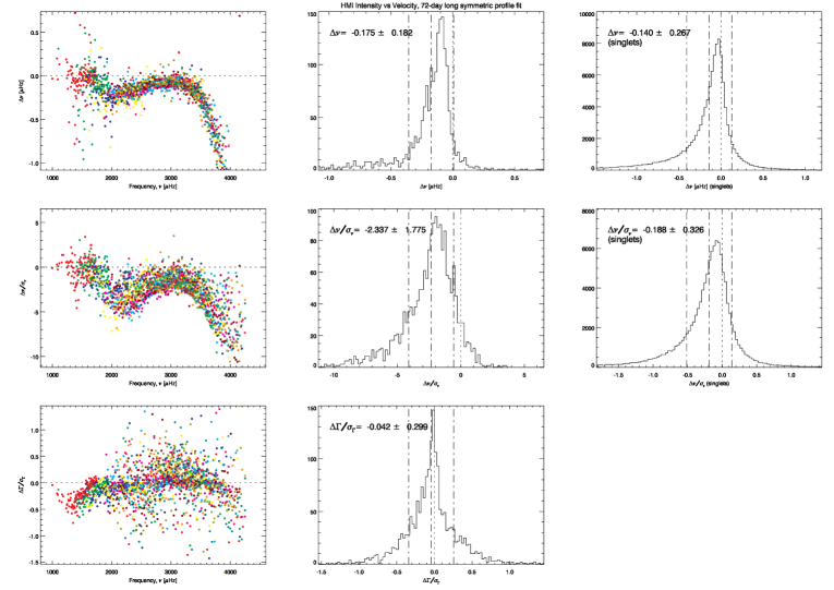
Figure 17: Comparison of mode characteristics derived from fitting a 72-day long time series, as shown in Fig. 15, but resulting from fitting co-eval intensity and velocity time series, using in both cases a symmetric peak profile ($\alpha_{n,\ell}=0$). The frequency differences become significant and systematic when ignoring the mode profile asymmetry.

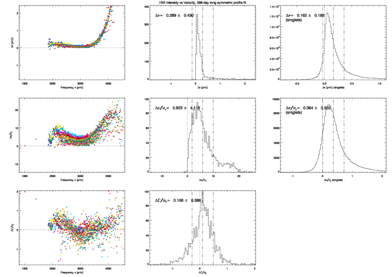
Figure 18: Comparison of mode characteristics derived from fitting a 288-day long time series, as shown in Fig. 17, namely resulting from fitting co-eval intensity and velocity time series, using in both cases a symmetric peak profile ($\alpha_{n,\ell}=0$). The frequency differences are quite significant and systematic when ignoring the mode profile asymmetry.

Since I also fitted the data using a symmetric mode profile, I can do the exact same comparison but using mode characteristics derived from fitting a symmetric profile for either type of observations or length of time series. This comparison is presented in Figs 17 and 18 and systematic differences with skewed distributions are clearly visible.

Table 3 summarizes the comparisons and lists the mean and standard deviation around the mean of the differences or scaled differences. Comparing results from fitting symmetric profiles demonstrate clearly the need to include the asymmetry of the mode profile at low and intermediate degrees, and not just at high degrees. While the differences are not very large in themselves, especially for 72-day long times series singlets, they rise to the $2.3$ and $5.9\,\sigma$ levels for multiplets derived from 72-day and 288-day long time series respectively, but more to the point these differences clearly show systematic trends. Close scrutiny of the table indicates a small residual bias in frequency differences from fitting co-eval velocity and intensity, even when using an asymmetric profile. It may well be that this small bias results from some remaining inadequacy in the fitting methodologies worth pursuing. This should not distract from the main conclusion that the inclusion of the asymmetry is key in the determination of accurate mode characteristics that are consistent whether measured using their manifestation from intensity or velocity fluctuations.

3 Conclusions

Initial results from fitting HMI intensity observations using my state of the art fitting methodology and including the mode profile asymmetry show a remarkable agreement of the derived mode characteristics with the corresponding values derived from co-eval velocity observations. Of course, the mode asymmetry for intensity is of opposite sign to the the mode asymmetry for velocity, as anticipated, and it is also larger in magnitude. The comparison of mode frequency and FWHM determinations based on intensity and velocity show no bias with a uniform normal distribution with a $0.3\,\sigma$ spread, and a very similar precision on the mode frequency. This being said, my attempt to validate various estimates of the leakage matrix for intensity shows residual inconsistencies that need to be resolved. I also show that despite these inconsistencies, the derived modes characteristics do not seem to be affected in any systematic way, at least for the precision resulting from fitting 72-day or 288-day long time series. Fitting a much longer time series may point to systematic errors associated to the leakage matrix determination.

One of the main drawbacks of intensity observations is the much higher noise level at low frequencies than in velocity observations. For reasons that I have yet to understand, and thus warrant more work, my fitting methodology was able to determine low-order low-frequency singlets for the shorter time series, but not for the longer one. One simple explanation could be that the sanity rejection is not stringent enough and the fitted modes are just realization noise spikes that happened to coincide with a mode frequency and should be ignored. The principle that I have followed, namely to fit time series of different lengths, again proves to be a good idea. I expect to fit additional HMI intensity data as they become available and fit them using the factor progression I have used for the velocity observations, namely fitting time series that are 36-day, 72-day, 144-day, 288-day, etc… long.

Finally, comparisons of mode characteristics derived by fitting a symmetric mode profile show unequivocally the systematic bias introduced in the mode frequency determinations by ignoring the asymmetry. Also, by fitting additional HMI intensity observations that will cover most of Cycle 24, I will be able to confirm whether the mode asymmetry both for intensity and velocity changes with solar activity, changes that I see in my fitting of velocity observations, but is not seen by others. Indeed, co-eval intensity and velocity derived frequencies ought to agree consistently independently of the solar activity level. Therefore, a change in the velocity-derived asymmetry will have to be matched by a change in the intensity-derived asymmetry, although of opposite sign and different in magnitude, to keep the derived frequencies in agreement.

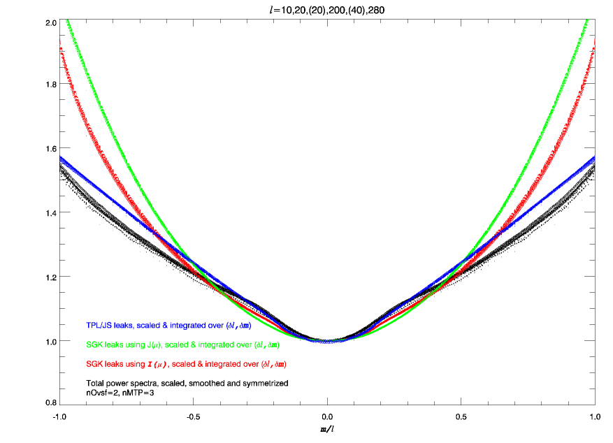
Figure 3: Direct comparison of the profiles shown in Fig. 2, with the size of the symbol proportional to $\ell$. Note that none of the leakage computations match the observed total power, nor do they duplicate correctly the distinctive “kink” near $m/\ell=0.25$ seen in the power profiles, although the case computed by me, using $I(\mu)$, displays a hint of a qualitatively similar kink.

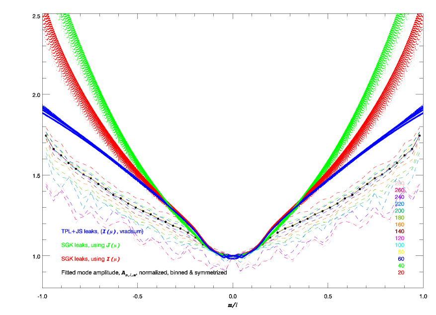
Figure 4: Comparison, like the one shown in Fig. 3, but using the fitted mode power amplitude, $A_{n,\ell,m}$ to estimate the normalized and symmetrized observed power distribution profile with respect to $m/\ell$ and shown as the connected black dots. The normalized values $\bar{Q}_{\ell,m}=\frac{C^{2}_{\ell,m}(0,0)}{C^{2}_{\ell,0}(0,0)}$,i.e., no summation on $(\delta\ell,\delta m)$, are shown with colored dots, with their size being proportional to $\ell$. The dash colored lines correspond to estimates of the observed power distribution profile, derived from measured $A_{n,\ell,m}$ but restricted to a given range in $\ell$ centered around a target $\ell$. Note that again none of the leakage computations match the mode profile power amplitude, nor do they duplicate correctly the distinctive “kink” seen in the observations, although the case computed by me and by the Stanford group, both using $I(\mu)$, displays a hint of a qualitatively similar kink.

Length	Start Time	End Time	Duty Cycle (%)
(day)	(TAI)	(TAI)	Velocity	Intensity
72	2010.04.30 00:00	2010.07.10 23:59	99.991	99.660
	2010.07.11 00:00	2010.09.20 23:59	99.466	98.328
	2010.09.21 00:00	2010.12.01 23:59	99.468	97.078
	2010.12.02 00:00	2011.02.11 23:59	99.462	98.958
288	2010.07.11 00:00	2011.04.24 23:59	99.366	97.774

Table 1: Length, start and end time of fitted time series and their respective duty cycles. The duty cycles of the velocities time series correspond to the gap filled ones, the duty cycles of the intensity time series correspond to the raw series.

Fitted profile	Asymmetric
Time series length	72 days
Data type/Leakage	$V$/SU
Start time	2010.04.30	2010.07.11	2010.09.21	2010.12.02
No. of singlets	205,530	206,251	204,956	204,969
No. of multiplets	2,297	2,296	2,287	2,294
Data type/Leakage	$I$/SU
No. of singlets	149,420	148,457	146,072	147,952
No. of multiplets	1,679	1,669	1,649	1,675
Data type/Leakage	$I$/SGK
No. of singlets	145,793	145,020	142,612	144,266
No. of multiplets	1,662	1,678	1,657	1,661
Time series length	288 days
Start time	2010.07.11
Data type/Leakage	$V$/SU	$I$/SGK	$I_{\rm gf}$/SGK
No. of singlets	281,977	202,420	202,719
No. of multiplets	2,386	1,682	1,682
Fitted profile	Symmetric
Time series length	72 days
Data type/Leakage	$V$/SU
Start time	2010.04.30	2010.07.11	2010.09.21	2010.12.02
No. of singlets	206,227	206,265	203,374	204,858
No. of multiplets	2,287	2,285	2,278	2,281
Data type	$I$/SGK
No. of singlets	143,534	142,502	140,386	141,894
No. of multiplets	1,654	1,655	1,628	1,649
Time series length	288 days
Start time	2010.07.11
Data type/Leakage	$V$/SU	$I$/SGK
No. of singlets	282,787	196,639
No. of multiplets	2,389	1,670

Table 2: Number of fitted singlets and derived multiplets for different fitting cases.

Length	$\Delta\nu$	$\Delta\nu/\sigma_{\nu}$	$\Delta\Gamma/\sigma_{\Gamma}$	$\Delta\alpha/\sigma_{\alpha}$	Number of
[days]	[$\mu$Hz]				common modes
	Asymmetric fitting, $I$, different leakage matrices, i.e., SU vs SGK
72	0.000 $\pm$ 0.015	0.001 $\pm$ 0.017			142,704	singlets
	0.001 $\pm$ 0.014	0.001 $\pm$ 0.016			141,645
	0.000 $\pm$ 0.015	0.001 $\pm$ 0.016			139,598
	0.000 $\pm$ 0.015	0.000 $\pm$ 0.017			141,164
288	-0.000 $\pm$ 0.008	-0.000 $\pm$ 0.015			201,658
72	0.000 $\pm$ 0.029	0.004 $\pm$ 0.233	-0.023 $\pm$ 0.060	-0.001 $\pm$ 0.071	1,653	multiplets
	0.001 $\pm$ 0.021	0.025 $\pm$ 0.231	-0.021 $\pm$ 0.058	-0.002 $\pm$ 0.061	1,651
	0.001 $\pm$ 0.023	0.014 $\pm$ 0.235	-0.017 $\pm$ 0.059	-0.004 $\pm$ 0.065	1,633
	0.002 $\pm$ 0.032	0.017 $\pm$ 0.220	-0.019 $\pm$ 0.060	-0.001 $\pm$ 0.065	1,647
288	0.000 $\pm$ 0.006	-0.000 $\pm$ 0.113	0.017 $\pm$ 0.055	0.001 $\pm$ 0.043	1,679
	Asymmetric fitting, $I$, gap filled vs no gap filling
288	0.001 $\pm$ 0.013	0.001 $\pm$ 0.028			200,909	singlets
288	0.001 $\pm$ 0.006	0.023 $\pm$ 0.125	0.005 $\pm$ 0.035	0.005 $\pm$ 0.045	1,676	multiplets
	Asymmetric fitting, $I-V$
72	0.015 $\pm$ 0.236	0.014 $\pm$ 0.289			115,347	singlets
	0.015 $\pm$ 0.239	0.011 $\pm$ 0.298			115,299
	0.014 $\pm$ 0.238	0.011 $\pm$ 0.294			114,003
	0.012 $\pm$ 0.236	0.008 $\pm$ 0.292			114,621
288	0.021 $\pm$ 0.146	0.044 $\pm$ 0.296			191,979
72	0.044 $\pm$ 0.113	0.470 $\pm$ 0.893	-0.065 $\pm$ 0.401		1,637	multiplets
	0.049 $\pm$ 0.152	0.455 $\pm$ 0.854	-0.021 $\pm$ 0.354		1,658
	0.035 $\pm$ 0.096	0.434 $\pm$ 0.864	-0.033 $\pm$ 0.370		1,637
	0.033 $\pm$ 0.097	0.384 $\pm$ 0.844	-0.040 $\pm$ 0.369		1,640
288	0.028 $\pm$ 0.053	0.856 $\pm$ 1.075	-0.008 $\pm$ 0.482		1,674
	Symmetric fitting, $I-V$
72	0.118 $\pm$ 0.262	0.144 $\pm$ 0.312			114,581	singlets
	0.128 $\pm$ 0.265	0.153 $\pm$ 0.318			114,179
	0.124 $\pm$ 0.263	0.149 $\pm$ 0.315			112,974
	0.119 $\pm$ 0.261	0.146 $\pm$ 0.312			113,707
288	0.161 $\pm$ 0.193	0.343 $\pm$ 0.350			188,372
72	0.183 $\pm$ 0.225	2.133 $\pm$ 1.724	-0.040 $\pm$ 0.416		1,643	multiplets
	0.173 $\pm$ 0.175	2.233 $\pm$ 1.729	-0.004 $\pm$ 0.346		1,642
	0.165 $\pm$ 0.178	2.198 $\pm$ 1.780	-0.016 $\pm$ 0.375		1,621
	0.183 $\pm$ 0.226	2.120 $\pm$ 1.726	-0.019 $\pm$ 0.379		1,636
288	0.203 $\pm$ 0.256	5.395 $\pm$ 4.058	0.076 $\pm$ 0.483		1,662

Table 3: Mean and standard deviation around the mean of mode characteristics’ raw or scaled differences, computed using singlets or multiplets values, whether (i) using different leakage matrix evaluations, (ii) using gap filling or not, (iii) using intensity or co-eval velocity observations and fitting asymmetric profiles, and (iv) again using intensity or co-eval velocity observations but fitting symmetric profiles.

References

- Barban et al. (2004) Barban, C., Hill, F., & Kras, S. 2004, ApJ, 602, 516
- Corbard et al. (2013) Corbard, T., Salabert, D., Boumier, P., & Picard Team. 2013, in Astronomical Society of the Pacific Conference Series, Vol. 478, Fifty Years of Seismology of the Sun and Stars, ed. K. Jain, S. C. Tripathy, F. Hill, J. W. Leibacher, & A. A. Pevtsov, 151
- Couvidat et al. (2016) Couvidat, S., Schou, J., Hoeksema, J. T., Bogart, R. S., Bush, R. I., Duvall, T. L., Liu, Y., Norton, A. A., & Scherrer, P. H. 2016, Sol. Phys., 291, 1887
- Couvidat et al. (2012) Couvidat, S., Schou, J., Shine, R. A., Bush, R. I., Miles, J. W., Scherrer, P. H., & Rairden, R. L. 2012, Sol. Phys., 275, 285
- Duvall et al. (1993) Duvall, Jr., T. L., Jefferies, S. M., Harvey, J. W., Osaki, Y., & Pomerantz, M. A. 1993, ApJ, 410, 829
- Korzennik (2005) Korzennik, S. G. 2005, ApJ, 626, 585
- Korzennik (2008) Korzennik, S. G. 2008, in Journal of Physics Conference Series, Vol. 118, Journal of Physics Conference Series, 012082
- Korzennik (2013) Korzennik, S. G. 2013, in Astronomical Society of the Pacific Conference Series, Vol. 478, Fifty Years of Seismology of the Sun and Stars, ed. K. Jain, S. C. Tripathy, F. Hill, J. W. Leibacher, & A. A. Pevtsov, 137
- Korzennik et al. (2004) Korzennik, S. G., Rabello-Soares, M. C., & Schou, J. 2004, ApJ, 602, 481
- Oliviero et al. (2001) Oliviero, M., Severino, G., & Straus, T. 2001, in ESA Special Publication, Vol. 464, SOHO 10/GONG 2000 Workshop: Helio- and Asteroseismology at the Dawn of the Millennium, ed. A. Wilson & P. L. Pallé, 669–672
- Pierce & Slaughter (1977) Pierce, A. K. & Slaughter, C. D. 1977, Sol. Phys., 51, 25
- Salabert et al. (2013) Salabert, D., García, R. A., & Jiménez, A. 2013, in Astronomical Society of the Pacific Conference Series, Vol. 478, Fifty Years of Seismology of the Sun and Stars, ed. K. Jain, S. C. Tripathy, F. Hill, J. W. Leibacher, & A. A. Pevtsov, 145
- Schou (1999) Schou, J. 1999, ApJ, 523, L181
- Schou et al. (2012) Schou, J., Scherrer, P. H., Bush, R. I., Wachter, R., Couvidat, S., Rabello-Soares, M. C., Bogart, R. S., Hoeksema, J. T., Liu, Y., Duvall, T. L., Akin, D. J., Allard, B. A., Miles, J. W., Rairden, R., Shine, R. A., Tarbell, T. D., Title, A. M., Wolfson, C. J., Elmore, D. F., Norton, A. A., & Tomczyk, S. 2012, Sol. Phys., 275, 229
- Woodard (1984) Woodard, M. F. 1984, PhD thesis, University of California, San Diego.