Penalty Alternating Direction Methods
for Mixed-Integer Optimization:
A New View on Feasibility Pumps

Abstract.

Feasibility pumps are highly effective primal heuristics for mixed-integer linear and nonlinear optimization. However, despite their success in practice there are only few works considering their theoretical properties. We show that feasibility pumps can be seen as alternating direction methods applied to special reformulations of the original problem, inheriting the convergence theory of these methods. Moreover, we propose a novel penalty framework that encompasses this alternating direction method, which allows us to refrain from random perturbations that are applied in standard versions of feasibility pumps in case of failure. We present a convergence theory for the new penalty based alternating direction method and compare the new variant of the feasibility pump with existing versions in an extensive numerical study for mixed-integer linear and nonlinear problems.

Due to their practical relevance, mixed-integer nonlinear problems (MINLPs) form a very important class of optimization problems. One important part of successful algorithms for the solution of such problems is finding feasible solutions quickly. For this, typically heuristics are employed. These can be roughly divided into heuristics that improve known feasible solutions (e.g., local branching [25] or RINS [16]) and heuristics that construct feasible solutions from scratch. This article discusses a heuristic of the latter type: The algorithm of interest in this article is the so-called feasibility pump that has originally been proposed by [24] in [24] for MIPs and that has been extended by many other researchers, e.g., in [1, 2, 3, 6, 7, 17, 18, 26, 34, 19]. In addition, feasibility pumps have also been applied to MINLPs during the last years; see, e.g., [8, 4, 9, 14, 15, 39, 40]. A more detailed review of the literature about feasibility pumps is given in Section 1. For a comprehensive overview over primal heuristics for mixed-integer linear and nonlinear problems in general, we refer the interested reader to [5, 4] and the references therein.

In a nutshell, feasibility pumps work as follows: given an optimal solution of the continuous relaxation of the problem, the methods construct two sequences. The first one contains integer-feasible points, the second one contains points that are feasible w.r.t. the continuous relaxation. Thus, one has found an overall feasible point if these sequences converge to a common point. To escape from situations where the construction of the sequences gets stuck and thus do not converge to a common point, feasibility pumps usually incorporate randomized restarts.

The feasibility pumps described in the literature are difficult to analyze theoretically due to the use of random perturbations. These random perturbations are, however, crucial to the practical performance of the methods. The main object of the existing theoretical analysis is the idealized feasibility pump, i.e., the method without random perturbations. This is the method analyzed in the publications [17] and [6]. To be more specific, [17] show in [17] that idealized feasibility pumps are a special case of the Frank–Wolfe algorithm applied to a suitable chosen concave and nonsmooth merit function and [6] showed in [6] that idealized feasibility pumps can be seen as discrete versions of the proximal point algorithm. However, the analysis presented in both mentioned publications cannot be applied to feasibility pumps that use random perturbations. Recently, there has been progress in the understanding of the randomization step. In [19], the authors show that changing the randomization step can yield a method that, at least for certain instances, is guaranteed to produce feasible solutions with high probability.

Our approach is similar to these publications. We show that the idealized variant can be seen as an alternating direction method (ADM) applied to a special reformulation of the mixed-integer problem at hand. To this end, we extend the known theory on feasibility pumps by applying the convergence theory of general ADMs. We then go one step further: The necessity to use random perturbations comes from the need to escape from undesired points. We replace these random perturbations of the original feasibility pump by a penalty framework. This allows us to view feasibility pumps as penalty based alternating direction methods—a new class of optimization methods for which we also present convergence theory. In summary, we are able to give a convergence theory for a class of feasibility pumps that incorporates deterministic restart rules. Another advantage is that our method can be presented in a quite generic way that comprises both the case of mixed-integer linear and nonlinear problems.

We further give extensive computational results to show that our replacement of the random restarts also works well in practice. In particular, our method compares favorably with published variants of feasibility pumps for MIPs and MINLPs w.r.t. solution quality.

The paper is organized as follows: In Section 1 we review the main ingredients of feasibility pumps and give a more detailed literature survey. Afterward, we discuss general ADMs in Section 2 and show that idealized feasibility pumps can be seen as ADMs applied to certain equivalent reformulations of the original problem. In Section 3, we then present a penalty ADM, prove convergence results, and show how this new method can be used to obtain a novel feasibility pump algorithm that replaces random restarts with penalty parameter updates. In Section 4 we discuss important implementation issues and Section 5 finally presents an extensive computational study both for MIPs and MINLPs.

1. Feasibility Pumps

In this section we give an overview over feasibility pump algorithms for mixed-integer linear problems (MIPs) as well as for mixed-integer nonlinear problems (MINLPs). We start with the MIP case in Section 1.1 and afterward discuss generalizations for nonlinear problems in Section 1.2. General surveys on this topic can be found in [4] and [10].

1.1. Feasibility Pumps for Mixed-Integer Linear Problems

The feasibility pump has been introduced by [24] for binary MIPs and has been extended to general MIPs by [3]. The goal of the feasibility pump is to find a feasible point of a mixed-integer linear problem of the general form

$$\min_{x}\quad {c}^{\top}x$$ (1a)

s.t. $$Ax\geq b,$$ (1b)

$$x_{i}\in\mathds{Z}\quad\text{for all\ }i\in I,$$ (1c)

where $c\in\mathds{R}^{n}$, $b\in\mathds{R}^{m}$, $A\in\mathds{R}^{m\times n}$, and $\emptyset\neq I\subseteq\left\{{1,\dotsc,n}\right\}$. Moreover, we assume that variable bounds $l\leq x\leq u$ with $-\infty<l_{i}\leq u_{i}<\infty$ for all $i\in I$ are part of $Ax\geq b$. We refer to the polyhedron of the LP relaxation of (1) by $P$, i.e., $P=\{x\in\mathds{R}^{n}:Ax\geq b\}$. Throughout the paper we assume that $P\neq\emptyset$. The main idea of the feasibility pump is to create two sequences $(\bar{x}^{k})$ and $(\tilde{x}^{k})$ such that $\bar{x}^{k}\in P$ and $\tilde{x}^{k}$ is integer feasible, i.e., $\tilde{x}^{k}_{i}\in\mathds{Z}$ for all $i\in I$. In addition, the construction of the sequences is tailored to minimize the distance of the pairs $\bar{x}^{k}$ and $\tilde{x}^{k}$. The algorithm terminates after a given time, after an iteration limit has been reached, or if the distance is zero, i.e., $\bar{x}^{k}=\tilde{x}^{k}$. In the latter case, the algorithm terminates with an MIP-feasible point, i.e., a point that is both in $P$ and integer feasible. We now describe the method in detail for the case of $0$-$1$-MIPs, i.e., we replace $x_{i}\in\mathds{Z}$ by $x_{i}\in\left\{{0,1}\right\}$ in (1c). The initial point $\bar{x}^{0}$ is computed to be an optimal solution of the LP relaxation of (1), i.e., $\bar{x}^{0}\in\operatorname*{argmin}\{{c}^{\top}x:x\in P\}$, and the initial point $\tilde{x}^{0}$ of the other sequence is the rounding $\lceil\bar{x}^{0}\rfloor$ of the integer components of $\bar{x}^{0}$. Note that the rounding operator $\lceil\cdot\rfloor$ only rounds integer components, i.e.,

$$\lceil x_{i}\rfloor\mathrel{\mathop{:}}=\begin{cases}\lfloor x_{i}+0.5\rfloor,&\text{if }i\in I,\\ x_{i},&\text{otherwise}.\end{cases}$$

From then on, in each iteration $k$ the new iterate $\bar{x}^{k+1}$ is the nearest point (w.r.t. the integer components) to $\tilde{x}^{k}$ in the $\ell_{1}$ norm, i.e.,

$$\bar{x}^{k+1}\in\operatorname*{argmin}\{\lVert x_{I}-\tilde{x}_{I}^{k}\rVert_{1}:x\in P\}$$

and $\tilde{x}^{k+1}\mathrel{\mathop{:}}=\lceil\bar{x}^{k+1}\rfloor$. Here and in what follows, $x_{I}$ denotes the sub-vector of $x$ only consisting of the components indicated by the index set $I$. After every rounding step a cycle and a stalling test decides whether a random perturbation of the integer part of $\tilde{x}^{k}$ is applied. The details can be found in [24, 3]. A formal listing of the basic feasibility pump for binary MIPs is given in Algorithm 1.

Algorithm 1 The basic feasibility pump for $0$-$1$-MIPs

1:  Compute $\bar{x}^{0}\in\operatorname*{argmin}\{{c}^{\top}x:x\in P\}$.

2:  if $\bar{x}^{0}$ is integer feasible then

3:     return  $\bar{x}^{0}$

4:  end if

5:  Set $\tilde{x}^{0}=\lceil\bar{x}^{0}\rfloor$ and $k\leftarrow 0$.

6:  while not termination condition do

7:     Compute $\bar{x}^{k+1}\in\operatorname*{argmin}\{\lVert x_{I}-\tilde{x}_{I}^{k}\rVert_{1}:x\in P\}$.

8:     if $\bar{x}^{k+1}$ is integer feasible then

9:        return  $\bar{x}^{k+1}$

10:     end if

11:     Set $\tilde{x}^{k+1}=\lceil\bar{x}^{k+1}\rfloor$.

12:     if algorithm stalls or cycles then

13:        perturb $\tilde{x}^{k+1}$

14:     end if

15:     Set $k\leftarrow k+1$.

16:  end while

In what follows, Line 7 of Algorithm 1 is referred to as the projection step and Line 11 is called the rounding step. Note that the projection step can be written as a linear program by reformulating the $\ell_{1}$ norm objective as

$$\lVert x_{I}-\tilde{x}_{I}\rVert_{1}=\sum_{i\in I:\tilde{x}_{i}=0}x_{i}+\sum_{i\in I:\tilde{x}_{i}=1}(1-x_{i}).$$

This is also possible for general MIPs but then requires the introduction of auxiliary variables and constraints; see [3] for the details. The original feasibility pump is very successful in quickly finding feasible solutions.

However, these solutions are often of minor quality. Thus, improvements of the original version with the goal of developing variants of the feasibility pump that are comparable in running time as well as success rate and provide solutions of better quality are studied in many publications. [26] improved the rounding step by replacing the simple rounding $\tilde{x}^{k}=\lceil\bar{x}^{k}\rfloor$ with a procedure based on constraint propagation. Other strategies of improving the rounding step are given in [2], where simple rounding is replaced with rounding of different candidate points on a line segment between the solution of the projection step and the analytic center of the LP polyhedron, and in [7], where an integer line search is applied to find integer feasible points that are closer to $P$ than the points achieved by simple rounding. In contrast to these approaches, [1] improved the projection step in order to achieve feasible solutions of better quality by replacing the $\ell_{1}$ norm objective $\lVert x_{I}-\tilde{x}_{I}\rVert_{1}$ with a convex combination of this distance measure and the original objective function:

$$(1-\alpha)\lVert x_{I}-\tilde{x}_{I}\rVert_{1}+\alpha\beta{c}^{\top}x.$$

Here, $\alpha\in[0,1]$ is the convex combination parameter and $\beta\in\mathds{R}_{>0}$ is a problem data depending scaling parameter; see [1] for the details.

None of the papers cited so far contains any theoretical results on the feasibility pump. This situation changed with a remark in [23] noticing that the idealized feasibility pump for binary MIPs can be interpreted as a Frank–Wolfe algorithm (see [27]) applied to the minimization of a concave and nonsmooth objective function over a polyhedron. [17] seized this idea and proved this correspondence, yielding the first theoretical result for the feasibility pump. To be more precise, they used the result shown by [36] in [36] that the Frank–Wolfe algorithm applied to the above given situation terminates after a finite number of iterations and returns a so-called vertex stationary point of the problem. We discuss the relation of this result with our results in more detail in Section 2.1. In [18], [18] generalized their results to general MIPs. Another theoretical result is presented by [6] in [6], where it is shown that the idealized feasibility pump can be interpreted as a discrete version of the proximal point algorithm. We remark that both cited theoretical investigations only consider the case of idealized feasibility pumps, i.e., the variants of feasibility pumps without random perturbations used to handle cycling or stalling issues.

1.2. Feasibility Pumps for Mixed-Integer Nonlinear Problems

We now turn to feasibility pumps for mixed-integer nonlinear problems of the form

$$\min_{x}\quad f(x)$$ (2a)

s.t. $$h(x)\geq 0,$$ (2b)

$$x_{i}\in\mathds{Z}\cap[l_{i},u_{i}]\quad\text{for all\ }i\in I,$$ (2c)

where the objective function $f:\mathds{R}^{n}\to\mathds{R}$ and the constraints function $h:\mathds{R}^{n}\to\mathds{R}^{p}$ are continuous. The feasible set of the NLP relaxation is denoted by $\Omega^{\mathrm{r}}\mathrel{\mathop{:}}=\{x\in\mathds{R}^{n}:h(x)\geq 0\}$. Again, we assume that $\Omega^{\mathrm{r}}\neq\emptyset$ holds and that $\Omega^{\mathrm{r}}$ is compact. Lastly, we assume that all bounds on the discrete variables are finite, i.e., $-\infty<l_{i}\leq u_{i}<\infty$ for all $i\in I$. The MINLP (2) is said to be convex if $f$ and $-h$ are convex.

For convex problems, the direct generalization of the feasibility pump for MIPs to MINLPs is given in [9]: the projection step LP is replaced by an NLP and the rounding step stays the same, i.e., $\tilde{x}^{k+1}\mathrel{\mathop{:}}=\lceil\bar{x}^{k+1}\rfloor$. Cycling and stalling issues are again handled by random perturbations of the integer components of $x$. Variants of this method are then deduced by modifying the rounding step and by replacing the $\ell_{1}$ with the $\ell_{2}$ norm in the projection step. The feasibility pump for convex MINLP proposed in [8] significantly differs from the version in [9] because it replaces the simple rounding step by a MIP relaxation of (2) that is successively tightened by adding outer approximation cuts (see [22]) based on the NLP feasible solutions obtained by solving the $\ell_{2}$ norm projection steps. [8] study two versions of their algorithm; a basic and an enhanced one. For their basic version it is shown that it cannot cycle if the LICQ holds for the NLP relaxation. For their enhanced version it is shown that it cannot cycle and that it is an exact method for solving convex MINLPs if all integer variables are bounded.

For nonconvex MINLPs the convergence results of [8] do not hold because the outer approximation cuts cannot be applied to the nonconvex NLP relaxation and because the projection step is now a nonconvex problem, which is too hard to be solved to global optimality in general. The article [15] is the first presentation of a feasibility pumps for nonconvex MINLPs. The above mentioned issues are “resolved” by solving the nonconvex projection step NLP via a multistart heuristic using local NLP solvers and the rounding step is realized by a MIP using outer approximation cuts if they are globally valid for the nonconvex problem. In the subsequent paper [14], [14] interpreted feasibility pumps for general nonconvex MINLPs as variants of successive projection methods (SPMs). Despite their strong similarity, the authors observe that typical feasibility pumps do not fall exactly into the class of SPMs, which is why their convergence theory is not applicable.

Finally, a generalization of the objective feasibility pump of [1] is given in [39, 40] for convex MINLP and [4] discusses some new algorithmic ideas for nonconvex MINLPs.

2. Alternating Direction Methods

In this section, we first briefly review classical alternating direction methods (ADMs) and afterward prove that idealized feasibility pumps, i.e., the basic feasibility pump (Algorithm 1) without random perturbations, can be seen as a special case of alternating direction methods. This gives new theoretical insights since the complete theory of ADMs can be applied to idealized feasibility pumps.

To this end, we consider the general problem

$$\min_{x,y}\quad f(x,y)$$ (3a)

s.t. $$g(x,y)=0,\quad h(x,y)\geq 0,$$ (3b)

$$x\in X,\quad y\in Y,$$ (3c)

for which we make the following assumption:

Assumption 1.

The objective function $f:\mathds{R}^{n_{x}+n_{y}}\to\mathds{R}$ and the constraint functions $g:\mathds{R}^{n_{x}+n_{y}}\to\mathds{R}^{m}$, $h:\mathds{R}^{n_{x}+n_{y}}\to\mathds{R}^{p}$ are continuous and the sets $X$ and $Y$ are non-empty and compact.

The feasible set is denoted by $\Omega$, i.e.,

$$\Omega=\{(x,y)\in X\times Y:g(x,y)=0,\ h(x,y)\geq 0\}\subseteq X\times Y,$$

and the corresponding projections onto $X$ and $Y$ are denoted by $\Omega_{X}$ and $\Omega_{Y}$, respectively. Classical alternating direction methods are extensions of Lagrangian methods and have been originally proposed in [28] and [30]. More recently, ADM-type methods have seen a resurgence; see, e.g., [11] for a general overview and [29] for an application of ADMs to nonconvex MINLPs from gas transport including heat power constraints. The latter application also provided the motivation for this article. ADMs solve Problem (3) by solving two simpler problems: Given an iterate $(x^{k},y^{k})$ they solve Problem (3) for $y$ fixed to $y^{k}$ into the direction of $x$, yielding a new $x$-iterate $x^{k+1}$. Afterward, $x$ is fixed to $x^{k+1}$ and Problem (3) is solved into the direction of $y$, yielding a new $y$-iterate $y^{k+1}$. A formal listing is given in Algorithm 2. Note that we do not state a practical termination criterion in Algorithm 2 in order to facilitate a more streamlined analysis. For the implementation details we refer to Section 4.

Algorithm 2 A Standard Alternating Direction Method

1:  Choose initial values $(x^{0},y^{0})\in X\times Y$.

2:  for $k=0,1,\dotsc$ do

3:     Compute

$$x^{k+1}\in\operatorname*{argmin}_{x}\{f(x,y^{k}):g(x,y^{k})=0,\ h(x,y^{k})\geq 0,\ x\in X\}.$$

4:     Compute

$$y^{k+1}\in\operatorname*{argmin}_{y}\{f(x^{k+1},y):g(x^{k+1},y)=0,\ h(x^{k+1},y)\geq 0,\ y\in Y\}.$$

5:     Set $k\leftarrow k+1$.

6:  end for

If the optimization problem in Line 3 or Line 4 of Algorithm 2 has a unique solution for all $k$, it is known that ADMs converge to so-called partial minima of Problem (3), i.e., to points $(x^{*},y^{*})\in\Omega$ for which

$$f(x^{*},y^{*})\leq f(x,y^{*}) \quad\text{for all }(x,y^{*})\in\Omega,$$

$$f(x^{*},y^{*})\leq f(x^{*},y) \quad\text{for all }(x^{*},y)\in\Omega$$

holds; see [31] for the following result:

Theorem 2.1.

Let ${\left\{(x^{i},y^{i})\right\}}_{i=0}^{\infty}$ be a sequence with $(x^{i+1},y^{i+1})\in\Theta(x^{i},y^{i})$, where

$$\Theta(x^{i},y^{i})\mathrel{\mathop{:}}=\{(x^{*},y^{*}):\forall x\in X.\ f(x^{*},y^{i})\leq f(x,y^{i});\ \forall y\in Y.\ f(x^{*},y^{*})\leq f(x^{*},y)\}.$$

Suppose that Assumption 1 holds and that the solution of the first optimization problem is always unique. Then every convergent subsequence of ${\left\{(x^{i},y^{i})\right\}}_{i=0}^{\infty}$ converges to a partial minimum. For two limit points $z,z^{\prime}$ of such subsequences it holds that $f(z)=f(z^{\prime})$.

Stronger results can be obtained if additional assumptions are made on $f$ and $\Omega$: If $f$ is continuously differentiable, Algorithm 2 converges to a stationary point (in the classical sense of nonlinear optimization). If, in addition, $f$ and $\Omega$ are convex it is easy to show that partial minimizers are also global minimizers of Problem (3). For more details on the convergence theory of classical ADMs, see [31] as well as [41].

2.1. Feasibility Pumps as ADMs

Recall that the basic feasibility pump algorithm 1 tries to find a feasible solution for the binary variant of MIP (1). We now consider the idealized feasibility pump, i.e., we omit the perturbation step in Line 13 of Algorithm 1, and show that the idealized feasibility pump is a special case of the ADM (Algorithm 2) applied to a certain reformulation of MIP (1). To this end, we duplicate the variables $x_{I}$ using the new variable vector $y\in\left\{{0,1}\right\}^{I}$, yielding

$$\min_{x,y}\quad {c}^{\top}x$$

s.t. $$x\in X\mathrel{\mathop{:}}=\{x\in\mathds{R}^{n}:Ax\geq b,\ x_{I}\in{[0,1]}^{I}\},$$

$$y\in Y\mathrel{\mathop{:}}=\left\{{0,1}\right\}^{I},\quad g(x,y)=x_{I}-y=0,$$

which is obviously equivalent to the original MIP. Note that, compared to the general problem (3), we do not explicitly require the inequality constraints vector $h$. The feasibility pump is only interested in feasibility and thus ignores the objective function. By deleting the objective from the reformulated model and instead moving an $\ell_{1}$ penalty term of the coupling condition $y=x_{I}$ into the objective, we obtain

$$\min_{x,y}\quad \lVert x_{I}-y\rVert_{1}$$ (4a)

s.t. $$x\in X\mathrel{\mathop{:}}=\{x\in\mathds{R}^{n}:Ax\geq b,\ x_{I}\in{[0,1]}^{I}\},\quad y\in Y\mathrel{\mathop{:}}=\left\{{0,1}\right\}^{I}.$$ (4b)

If we define initial values $(x^{0},y^{0})$ by $x^{0}\mathrel{\mathop{:}}=\operatorname*{argmin}\{{c}^{\top}x:x\in X\}$ and $y^{0}\mathrel{\mathop{:}}=\lceil x^{0}\rfloor$, it can be easily seen that solving Problem (4) with the ADM algorithm 2 exactly corresponds to the idealized feasibility pump algorithm. To be more precise, finding the new $x$-iterate within the ADM coincides with the projection step and finding the new $y$-iterate corresponds to the rounding step.

In the context of Algorithm 2, we say that the sequence of iterates ${z^{k}}$ cycles if there exists an iteration $k$ and an $l\geq 2$ with $z^{k}=z^{k+l}$. Next, we prove that the ADM cannot cycle and thus terminates after a finite number of iterations. To this end, we make the following observations: First, $X$ and $Y$ in (4) are non-empty and compact sets. Second, we can assume uniqueness of the rounding step by resolving tie-breaks choosing lexicographically minimal solutions. Thus, by using that norms are continuous, we have the following result.

Lemma 2.2.

Algorithm 2 does not cycle.

Proof.

Assume the contrary, i.e., there exists an iteration $k$ and an $l\geq 2$ such that $z^{k},z^{k+1},\dotsc,z^{k+l}=z^{k}$. Since $f(x^{k+1},y^{k+1})\leq f(x^{k+1},y^{k})\leq f(x^{k},y^{k})$ holds for all iterations $k$ we directly see that $f(z^{k})=f(z^{k+1})=\dotsb=f(z^{k+l-1})$ holds. This, however, implies that $z^{k}$ is already a partial minimum at which the algorithm stops. ∎

We note that this lemma is equivalent to Proposition 1 of [17]. There, the authors show that the idealized feasibility pump for binary MIPs is equivalent to the Frank–Wolfe algorithm (using an unitary stepsize) applied to the problem

$$\min_{x\in P}\quad\sum_{i\in I}\min\left\{{x_{i},1-x_{i}}\right\},$$ (5)

where the objective function is a concave and nonsmooth merit function for measuring integrality. Applying the convergence theory from [36] then also yields finite termination at so-called vertex stationary points. Since we have now proven that the ADM (Algorithm 2) applied to (4) is equivalent to the above mentioned special case of the Frank–Wolfe method, we have also shown that partial minima of Problem (4) are exactly the vertex stationary points of Problem (5).

From the theory reported above and the last lemma we can directly deduce the following convergence theorem for the idealized feasibility pump.

Theorem 2.3.

The idealized feasibility pump terminates at a partial minimum $(x^{*},y^{*})$ of Problem (4) after a finite number of iterations. If the partial minimum $(x^{*},y^{*})$ has objective value $\lVert x^{*}_{I}-y^{*}\rVert_{1}=0$, the point $(x^{*},y^{*})$ is feasible for the MIP (1).

This theorem also gives us a new view of the random perturbation steps of feasibility pump algorithms: They can be interpreted as an attempt to escape from non-integral partial optima of Problem (4).

So far, we have only discussed the case of binary MIPs. However, our theory is still applicable as long as the optimization problems in Line 3 and 4 of Algorithm 2 are solved to global optimality. This is a realistic assumption for convex MINLPs of type (2). The suitable generalization of Problem (4) for this problem class reads

$$\min_{x,y}\quad \lVert x_{I}-y\rVert_{1}$$ (6a)

s.t. $$x\in X\mathrel{\mathop{:}}=\{x\in\mathds{R}^{n}:h(x)\geq 0,x_{I}\in{[0,1]}^{I}\},\quad y\in Y\mathrel{\mathop{:}}=\left\{{0,1}\right\}^{I}.$$ (6b)

We note that the resulting ADM is exactly the method presented in [9]. Using the same techniques as above, we get the following convergence theorem for the idealized feasibility pump for convex MINLP.

Theorem 2.4.

The idealized feasibility pump for convex MINLP (2) is equivalent to the ADM algorithm 2 applied to Problem (6). Thus, it terminates at a partial minimum $(x^{*},y^{*})$ of Problem (6) after a finite number of iterations. If this partial minimum has objective value $\lVert x^{*}_{I}-y^{*}\rVert_{1}=0$, the point $(x^{*},y^{*})$ is feasible for the convex MINLP (2).

We close this section with two remarks. First, we note that we presented the results in this section for binary MI(NL)Ps only for improving readability. The extension to general mixed-integer problems is straightforward; see Section 4 for the details. Second, we again want to highlight that the theoretical results presented in this section only hold if the optimization problems in Line 3 and 4 of Algorithm 2 are solved to global optimality. Since this is typically not possible for general nonconvex MINLPs, the results are only practically valid for convex mixed-integer problems.

3. The Penalty Alternating Direction Method

In this section we first present a new penalty alternating direction method in Section 3.1 and afterward prove the convergence results in Section 3.2. Finally, in Section 3.3 we show how the new method can be used to obtain a novel feasibility pump algorithm for general mixed-integer optimization. This new penalty alternating direction method based feasibility pump replaces random perturbations with a theoretically analyzable penalty framework for escaping from undesired intermediate points. Thus, the complete theory presented for the new method also applies to the new feasibility pump variant.

3.1. The Algorithm

We now present the novel weighted $\ell_{1}$ penalty method based on the classical ADM framework given in Section 2. To this end, we define the $\ell_{1}$ penalty function

$$\phi_{1}(x,y;\mu,\rho)\mathrel{\mathop{:}}=f(x,y)+\sum_{i=1}^{m}\mu_{i}\mathchoice{\left\lvert g_{i}(x,y)\right\rvert}{\lvert g_{i}(x,y)\rvert}{\lvert g_{i}(x,y)\rvert}{\lvert g_{i}(x,y)\rvert}+\sum_{i=1}^{p}\rho_{i}{[h_{i}(x,y)]}^{-},$$

where ${[\alpha]}^{-}\mathrel{\mathop{:}}=\max\left\{0,-\alpha\right\}$ holds and $\mu={(\mu_{i})}_{i=1}^{m},\rho={(\rho_{i})}_{i=1}^{p}\geq 0$ are the penalty parameters for the equality and inequality constraints. Note that we allow for different penalty parameters for the constraints instead of a single penalty parameter as it is often the case for penalty methods.

The penalty ADM now proceeds as follows. Given a starting point and initial values for all penalty parameters, the alternating direction method of Algorithm 2 is used to compute a partial minimum of the penalty problem

$$\min_{x,y}\quad\phi_{1}(x,y;\mu,\rho)\quad\text{s.t.}\quad x\in X,\ y\in Y.$$ (7)

Afterward, the penalty parameters are updated and the next penalty problem is solved to partial minimality. Thus, the algorithm produces a sequence of partial minima of a sequence of penalty problems of type (7). More formally, the method is specified in Algorithm 3.

Algorithm 3 The $\ell_{1}$ Penalty Alternating Direction Method

1:  Choose initial values $(x^{0,0},y^{0,0})\in X\times Y$ and penalty parameters $\mu^{0},\rho^{0}\geq 0$.

2:  for $k=0,1,\dotsc$ do

3:     Set $l=0$.

4:     while $(x^{k,l},y^{k,l})$ is not a partial minimum of (7) with $\mu=\mu^{k}$ and $\rho=\rho^{k}$ do

5:        Compute $x^{k,l+1}\in\operatorname*{argmin}_{x}\{\phi_{1}(x,y^{k,l};\mu^{k},\rho^{k}):x\in X\}$.

6:        Compute $y^{k,l+1}\in\operatorname*{argmin}_{y}\{\phi_{1}(x^{k,l+1},y;\mu^{k},\rho^{k}):y\in Y\}$.

7:        Set $l\leftarrow l+1$.

8:     end while

9:     Choose new penalty parameters $\mu^{k+1}\geq\mu^{k}$ and $\rho^{k+1}\geq\rho^{k}$.

10:  end for

3.2. Convergence Theory

We now present the convergence results for the penalty ADM algorithm 3. We start by proving that partial minima of the penalty problems are partial minima of the original problem if they are feasible.

Lemma 3.1.

Assume that $(x^{*},y^{*})$ is a partial minimum of $\phi_{1}(x,y;\mu,\rho)$ for arbitrary but fixed $\mu,\rho\geq 0$ and let $(x^{*},y^{*})$ be feasible for Problem (3). Then $(x^{*},y^{*})$ is a partial minimum of Problem (3).

Proof.

Let $x\in X$ such that $(x,y^{*})$ is feasible for Problem (3). Then it holds

$$f(x,y^{*}) =f(x,y^{*})+\sum_{i=1}^{m}\mu_{i}\mathchoice{\left\lvert g_{i}(x,y^{*})\right\rvert}{\lvert g_{i}(x,y^{*})\rvert}{\lvert g_{i}(x,y^{*})\rvert}{\lvert g_{i}(x,y^{*})\rvert}+\sum_{i=1}^{p}\rho_{i}{[h_{i}(x,y^{*})]}^{-}$$

$$=\phi_{1}(x,y^{*};\mu,\rho)\geq\phi_{1}(x^{*},y^{*};\mu,\rho)$$

$$=f(x^{*},y^{*})+\sum_{i=1}^{m}\mu_{i}\mathchoice{\left\lvert g_{i}(x^{*},y^{*})\right\rvert}{\lvert g_{i}(x^{*},y^{*})\rvert}{\lvert g_{i}(x^{*},y^{*})\rvert}{\lvert g_{i}(x^{*},y^{*})\rvert}+\sum_{i=1}^{p}\rho_{i}{[h_{i}(x^{*},y^{*})]}^{-}$$

$$=f(x^{*},y^{*}).$$

The analogous inequality holds for all $y\in Y$ such that $(x^{*},y)$ is feasible. Thus, $(x^{*},y^{*})$ is a partial minimum of Problem (3). ∎

For the next theorem we need some more notation. Let $\chi$ be the $\ell_{1}$ feasibility measure of Problem (3), which we define as

$$\chi(x,y)\mathrel{\mathop{:}}=\sum_{i=1}^{m}\mathchoice{\left\lvert g_{i}(x,y)\right\rvert}{\lvert g_{i}(x,y)\rvert}{\lvert g_{i}(x,y)\rvert}{\lvert g_{i}(x,y)\rvert}+\sum_{i=1}^{p}{[h_{i}(x,y)]}^{-}.$$

Obviously, $\chi(x,y)\geq 0$ holds and $\chi(x,y)=0$ if and only if $(x,y)$ is feasible w.r.t. $g$ and $h$. Moreover, we define the weighted $\ell_{1}$ feasibility measure as

$$\chi_{\mu,\rho}(x,y)\mathrel{\mathop{:}}=\sum_{i=1}^{m}\mu_{i}\mathchoice{\left\lvert g_{i}(x,y)\right\rvert}{\lvert g_{i}(x,y)\rvert}{\lvert g_{i}(x,y)\rvert}{\lvert g_{i}(x,y)\rvert}+\sum_{i=1}^{p}\rho_{i}{[h_{i}(x,y)]}^{-},$$

i.e., our $\ell_{1}$ penalty function can be stated as

$$\phi_{1}(x,y;\mu,\rho)=f(x,y)+\chi_{\mu,\rho}(x,y).$$

The next theorem states that the sequence of partial minima of the iteratively solved penalty problems converges to a partial minimum of $\chi_{\mu,\rho}$.

Lemma 3.2.

Suppose that Assumption 1 holds and that $\mu^{k}_{i}\nearrow\infty$ for all $i=1,\dotsc,m$ and $\rho^{k}_{i}\nearrow\infty$ for all $i=1,\dotsc,p$. Moreover, let $(x^{k},y^{k})$ be a sequence of partial minima of (7) (for $\mu=\mu^{k}$ and $\rho=\rho^{k}$) generated by Algorithm 3 with $(x^{k},y^{k})\to(x^{*},y^{*})$. Then there exist weights $\bar{\mu},\bar{\rho}\geq 0$ such that $(x^{*},y^{*})$ is a partial minimizer of the feasibility measure $\chi_{\bar{\mu},\bar{\rho}}$.

Proof.

Let $(x^{k},y^{k})$ be a partial minimizer of $\phi_{1}(x,y;\mu^{k},\rho^{k})$, i.e.,

$$\phi_{1}(x,y^{k};\mu^{k},\rho^{k})\geq\phi_{1}(x^{k},y^{k};\mu^{k},\rho^{k}) \quad\text{for all }x\in X,$$

$$\phi_{1}(x^{k},y;\mu^{k},\rho^{k})\geq\phi_{1}(x^{k},y^{k};\mu^{k},\rho^{k}) \quad\text{for all }y\in Y,$$

which is equivalent to

$$\begin{split}&f(x,y^{k})+\sum_{i=1}^{m}\mu_{i}^{k}\mathchoice{\left\lvert g_{i}(x,y^{k})\right\rvert}{\lvert g_{i}(x,y^{k})\rvert}{\lvert g_{i}(x,y^{k})\rvert}{\lvert g_{i}(x,y^{k})\rvert}+\sum_{i=1}^{p}\rho_{i}^{k}{[h_{i}(x,y^{k})]}^{-}\\ \geq\ &f(x^{k},y^{k})+\sum_{i=1}^{m}\mu_{i}^{k}\mathchoice{\left\lvert g_{i}(x^{k},y^{k})\right\rvert}{\lvert g_{i}(x^{k},y^{k})\rvert}{\lvert g_{i}(x^{k},y^{k})\rvert}{\lvert g_{i}(x^{k},y^{k})\rvert}+\sum_{i=1}^{p}\rho_{i}^{k}{[h_{i}(x^{k},y^{k})]}^{-}\end{split}$$ (8)

for all $x\in X$ and

$$\begin{split}&f(x^{k},y)+\sum_{i=1}^{m}\mu_{i}^{k}\mathchoice{\left\lvert g_{i}(x^{k},y)\right\rvert}{\lvert g_{i}(x^{k},y)\rvert}{\lvert g_{i}(x^{k},y)\rvert}{\lvert g_{i}(x^{k},y)\rvert}+\sum_{i=1}^{p}\rho_{i}^{k}{[h_{i}(x^{k},y)]}^{-}\\ \geq\ &f(x^{k},y^{k})+\sum_{i=1}^{m}\mu_{i}^{k}\mathchoice{\left\lvert g_{i}(x^{k},y^{k})\right\rvert}{\lvert g_{i}(x^{k},y^{k})\rvert}{\lvert g_{i}(x^{k},y^{k})\rvert}{\lvert g_{i}(x^{k},y^{k})\rvert}+\sum_{i=1}^{p}\rho_{i}^{k}{[h_{i}(x^{k},y^{k})]}^{-}\end{split}$$ (9)

for all $y\in Y$. The sequence $(\mu^{k},\rho^{k})\subseteq\mathds{R}^{m+p}$ is unbounded but the normalized sequence

$$\frac{(\mu^{k},\rho^{k})}{\lVert(\mu^{k},\rho^{k})\rVert}\subseteq\mathds{R}^{m+p},$$

is bounded. Thus, there exists a subsequence (indexed by $l$) of the normalized sequence such that

$$\frac{(\mu^{l},\rho^{l})}{\lVert(\mu^{l},\rho^{l})\rVert}\to(\bar{\mu},\bar{\rho})\quad\text{for }l\to\infty.$$

Division of (8) and (9) by $\lVert(\mu^{l},\rho^{l})\rVert$ yields

$$\frac{1}{\lVert(\mu^{l},\rho^{l})\rVert}f(x,y^{l})+\sum_{i=1}^{m}\frac{\mu_{i}^{l}}{\lVert(\mu^{l},\rho^{l})\rVert}\mathchoice{\left\lvert g_{i}(x,y^{l})\right\rvert}{\lvert g_{i}(x,y^{l})\rvert}{\lvert g_{i}(x,y^{l})\rvert}{\lvert g_{i}(x,y^{l})\rvert}+\sum_{i=1}^{p}\frac{\rho_{i}^{l}}{\lVert(\mu^{l},\rho^{l})\rVert}{[h_{i}(x,y^{l})]}^{-}$$

$$\geq\ \frac{1}{\lVert(\mu^{l},\rho^{l})\rVert}f(x^{l},y^{l})+\sum_{i=1}^{m}\frac{\mu_{i}^{l}}{\lVert(\mu^{l},\rho^{l})\rVert}\mathchoice{\left\lvert g_{i}(x^{l},y^{l})\right\rvert}{\lvert g_{i}(x^{l},y^{l})\rvert}{\lvert g_{i}(x^{l},y^{l})\rvert}{\lvert g_{i}(x^{l},y^{l})\rvert}+\sum_{i=1}^{p}\frac{\rho_{i}^{l}}{\lVert(\mu^{l},\rho^{l})\rVert}{[h_{i}(x^{l},y^{l})]}^{-}$$

for all $x\in X$ and

$$\frac{1}{\lVert(\mu^{l},\rho^{l})\rVert}f(x^{l},y)+\sum_{i=1}^{m}\frac{\mu_{i}^{l}}{\lVert(\mu^{l},\rho^{l})\rVert}\mathchoice{\left\lvert g_{i}(x^{l},y)\right\rvert}{\lvert g_{i}(x^{l},y)\rvert}{\lvert g_{i}(x^{l},y)\rvert}{\lvert g_{i}(x^{l},y)\rvert}+\sum_{i=1}^{p}\frac{\rho_{i}^{l}}{\lVert(\mu^{l},\rho^{l})\rVert}{[h_{i}(x^{l},y)]}^{-}$$

$$\geq\ \frac{1}{\lVert(\mu^{l},\rho^{l})\rVert}f(x^{l},y^{l})+\sum_{i=1}^{m}\frac{\mu_{i}^{l}}{\lVert(\mu^{l},\rho^{l})\rVert}\mathchoice{\left\lvert g_{i}(x^{l},y^{l})\right\rvert}{\lvert g_{i}(x^{l},y^{l})\rvert}{\lvert g_{i}(x^{l},y^{l})\rvert}{\lvert g_{i}(x^{l},y^{l})\rvert}+\sum_{i=1}^{p}\frac{\rho_{i}^{l}}{\lVert(\mu^{l},\rho^{l})\rVert}{[h_{i}(x^{l},y^{l})]}^{-}$$

for all $y\in Y$. Finally, by using that the limit preserves non-strict inequalities, linearity of the limit, and continuity of $f,g$, and $h$, for $l\to\infty$ we obtain

$$\sum_{i=1}^{m}\bar{\mu}_{i}\mathchoice{\left\lvert g_{i}(x,y^{*})\right\rvert}{\lvert g_{i}(x,y^{*})\rvert}{\lvert g_{i}(x,y^{*})\rvert}{\lvert g_{i}(x,y^{*})\rvert}+\sum_{i=1}^{p}\bar{\rho}_{i}{[h_{i}(x,y^{*})]}^{-}\geq\sum_{i=1}^{m}\bar{\mu}_{i}\mathchoice{\left\lvert g_{i}(x^{*},y^{*})\right\rvert}{\lvert g_{i}(x^{*},y^{*})\rvert}{\lvert g_{i}(x^{*},y^{*})\rvert}{\lvert g_{i}(x^{*},y^{*})\rvert}+\sum_{i=1}^{p}\bar{\rho}_{i}{[h_{i}(x^{*},y^{*})]}^{-}$$

for all $x\in X$ and

$$\sum_{i=1}^{m}\bar{\mu}_{i}\mathchoice{\left\lvert g_{i}(x^{*},y)\right\rvert}{\lvert g_{i}(x^{*},y)\rvert}{\lvert g_{i}(x^{*},y)\rvert}{\lvert g_{i}(x^{*},y)\rvert}+\sum_{i=1}^{p}\bar{\rho}_{i}{[h_{i}(x^{*},y)]}^{-}\geq\sum_{i=1}^{m}\bar{\mu}_{i}\mathchoice{\left\lvert g_{i}(x^{*},y^{*})\right\rvert}{\lvert g_{i}(x^{*},y^{*})\rvert}{\lvert g_{i}(x^{*},y^{*})\rvert}{\lvert g_{i}(x^{*},y^{*})\rvert}+\sum_{i=1}^{p}\bar{\rho}_{i}{[h_{i}(x^{*},y^{*})]}^{-}$$

for all $y\in Y$. This is equivalent to

$$\chi_{\bar{\mu},\bar{\rho}}(x,y^{*})\geq\chi_{\bar{\mu},\bar{\rho}}(x^{*},y^{*}) \quad\text{for all }x\in X,$$

$$\chi_{\bar{\mu},\bar{\rho}}(x^{*},y)\geq\chi_{\bar{\mu},\bar{\rho}}(x^{*},y^{*}) \quad\text{for all }y\in Y$$

and thus completes the proof. ∎

The two preceding lemmas now enable us to characterize the overall convergence behavior of the penalty ADM algorithm 3.

Theorem 3.3.

Suppose that Assumption 1 holds and that $\mu^{k}_{i}\nearrow\infty$ for all $i=1,\dotsc,m$ and $\rho^{k}_{i}\nearrow\infty$ for all $i=1,\dotsc,p$. Moreover, let $(x^{k},y^{k})$ be a sequence of partial minima of (7) (for $\mu=\mu^{k}$ and $\rho=\rho^{k}$) generated by Algorithm 3 with $(x^{k},y^{k})\to(x^{*},y^{*})$. Then there exist weights $\bar{\mu},\bar{\rho}\geq 0$ such that $(x^{*},y^{*})$ is a partial minimizer of the feasibility measure $\chi_{\bar{\mu},\bar{\rho}}$.

If, in addition, $(x^{*},y^{*})$ is feasible for the original problem (3), the following holds:

1. If $f$ is continuous, then $(x^{*},y^{*})$ is a partial minimum of (3).

2. If $f$ is continuously differentiable, then $(x^{*},y^{*})$ is a stationary point of (3).

3. If $f$ is continuously differentiable and $f$ and $\Omega$ are convex, then $(x^{*},y^{*})$ is a global optimum of (3).

Proof.

The first part always holds by Lemma 3.2. If, in addition, the obtained partial minimum of $\chi_{\bar{\mu},\bar{\rho}}$ satisfies $\chi_{\bar{\mu},\bar{\rho}}(x^{*},y^{*})=0$, we can apply Lemma 3.1 and obtain the statements a)–c). ∎

In the next theorem we generalize the classical result on the exactness of the $\ell_{1}$ penalty function (see, e.g., [33, 37]) to the setting of partial minima. For the ease of presentation, we state and prove this result only for the case without inequality constraints. However, the result can also be applied to problems including inequality constraints by using standard reformulation techniques to translate inequality constrained to equality constrained problems. Beforehand, we need two assumptions:

Assumption 2.

The objective function $f:X\times Y\to\mathds{R}$ of Problem (3) is locally Lipschitz continuous in the direction of $x$ and of $y$, i.e., for every $(x^{*},y^{*})\in\Omega$ there exists an open set $N(x^{*},y^{*})$ containing $(x^{*},y^{*})$ and a constant $L\geq 0$ such that

$$\mathchoice{\left\lvert f(x,y^{*})-f(x^{*},y^{*})\right\rvert}{\lvert f(x,y^{*})-f(x^{*},y^{*})\rvert}{\lvert f(x,y^{*})-f(x^{*},y^{*})\rvert}{\lvert f(x,y^{*})-f(x^{*},y^{*})\rvert}\leq L\lVert x-x^{*}\rVert \quad\text{for all }x\text{ with }(x,y^{*})\in N(x^{*},y^{*}),$$

$$\mathchoice{\left\lvert f(x^{*},y)-f(x^{*},y^{*})\right\rvert}{\lvert f(x^{*},y)-f(x^{*},y^{*})\rvert}{\lvert f(x^{*},y)-f(x^{*},y^{*})\rvert}{\lvert f(x^{*},y)-f(x^{*},y^{*})\rvert}\leq L\lVert y-y^{*}\rVert \quad\text{for all }y\text{ with }(x^{*},y)\in N(x^{*},y^{*}).$$

Note that if one set, say $Y$, is discrete, the corresponding condition is trivially satisfied. In this case any set of the form $(U,\left\{{y^{*}}\right\})$, where $U\subseteq X$ is an open neighborhood around $x^{*}$, is an open neighborhood around $(x^{*},y^{*})$.

Assumption 3.

For every constraint $g_{i},i=1,\dotsc,m$, there exists a constant $l_{i}>0$ such that

$$l_{i}\lVert x-x^{*}\rVert\leq\mathchoice{\left\lvert g_{i}(x,y^{*})-g_{i}(x^{*},y^{*})\right\rvert}{\lvert g_{i}(x,y^{*})-g_{i}(x^{*},y^{*})\rvert}{\lvert g_{i}(x,y^{*})-g_{i}(x^{*},y^{*})\rvert}{\lvert g_{i}(x,y^{*})-g_{i}(x^{*},y^{*})\rvert} \quad\text{for all }x\text{ with }(x,y^{*})\in N(x^{*},y^{*}),$$

$$l_{i}\lVert y-y^{*}\rVert\leq\mathchoice{\left\lvert g_{i}(x^{*},y)-g_{i}(x^{*},y^{*})\right\rvert}{\lvert g_{i}(x^{*},y)-g_{i}(x^{*},y^{*})\rvert}{\lvert g_{i}(x^{*},y)-g_{i}(x^{*},y^{*})\rvert}{\lvert g_{i}(x^{*},y)-g_{i}(x^{*},y^{*})\rvert} \quad\text{for all }y\text{ with }(x^{*},y)\in N(x^{*},y^{*}).$$

Note that in the case of existing directional derivatives of $g_{i}$, the latter assumption states that the directional derivatives of the $g_{i}$ both in the direction of $x$ and of $y$ are bounded away from zero. Before we state and proof the exactness theorem we briefly discuss the latter assumption. In the context of ADMs, the constraints $g(x,y)=0$ are mostly so-called copy constraints of the type

$$g(x,y)=A(x-y)=0$$

that are used to decompose the genuine problem formulation such that it fits into the framework of Problem (3); see, e.g., [38]. If the matrix $A$ is square and has full rank—as it is typically the case for copy constraints—the constraints $g$ are bi-Lipschitz and thus fulfill Assumption 3. Now, we are ready to state and prove the theorem on exactness of the $\ell_{1}$ penalty function w.r.t. partial minima.

Theorem 3.4.

Let $(x^{*},y^{*})$ be a partial minimizer of

$$\min_{x,y}\quad f(x,y)\quad\text{s.t.}\quad g(x,y)=0,\ x\in X,\ y\in Y,$$ (10)

and suppose that Assumptions 2 and 3 hold. Then there exists a constant $\bar{\mu}>0$ such that $(x^{*},y^{*})$ is a partial minimizer of

$$\min_{x,y}\quad\phi_{1}(x,y;\mu)\quad\text{s.t.}\quad x\in X,\ y\in Y$$

for all $\mu\geq\bar{\mu}$ and

$$\phi_{1}(x,y;\mu)\mathrel{\mathop{:}}=f(x,y)+\sum_{i=1}^{m}\mu_{i}\mathchoice{\left\lvert g_{i}(x,y)\right\rvert}{\lvert g_{i}(x,y)\rvert}{\lvert g_{i}(x,y)\rvert}{\lvert g_{i}(x,y)\rvert}.$$

Proof.

Since $(x^{*},y^{*})$ is a partial minimizer of Problem (10), it holds that

$$f(x,y^{*})\geq f(x^{*},y^{*}) \quad\text{for all }(x,y^{*})\in\Omega,$$ (11a)

$$f(x^{*},y)\geq f(x^{*},y^{*}) \quad\text{for all }(x^{*},y)\in\Omega,$$ (11b)

where $\Omega$ is the feasible region of Problem (10). First, assume that $(x,y^{*})$ is feasible for Problem (10). Using (11) we obtain

$$\phi_{1}(x^{*},y^{*};\mu) =f(x^{*},y^{*})+\sum_{i=1}^{m}\mu_{i}\mathchoice{\left\lvert g_{i}(x^{*},y^{*})\right\rvert}{\lvert g_{i}(x^{*},y^{*})\rvert}{\lvert g_{i}(x^{*},y^{*})\rvert}{\lvert g_{i}(x^{*},y^{*})\rvert}$$

$$=f(x^{*},y^{*})\leq f(x,y^{*})$$

$$=f(x,y^{*})+\sum_{i=1}^{m}\mu_{i}\mathchoice{\left\lvert g_{i}(x,y^{*})\right\rvert}{\lvert g_{i}(x,y^{*})\rvert}{\lvert g_{i}(x,y^{*})\rvert}{\lvert g_{i}(x,y^{*})\rvert}$$

$$=\phi_{1}(x,y^{*};\mu)$$

for all $\mu$. The inequality

$$\phi_{1}(x^{*},y^{*};\mu)\leq\phi_{1}(x^{*},y;\mu)$$

can be shown analogously assuming that $(x^{*},y)$ is feasible.

We now consider the case that $(x,y^{*})$ is not feasible for Problem (10). We set $\bar{\mu}\mathrel{\mathop{:}}=L/(m\bar{l})e>0$, where $\bar{l}\mathrel{\mathop{:}}=\min_{i=1,\dots,m}\left\{{l_{i}}\right\},e={(1,\dotsc,1)}^{\top}\in\mathds{R}^{m}$, and show that for all $\mu\geq\bar{\mu}$ the inequality

$$f(x,y^{*})+\sum_{i=1}^{m}\mu_{i}\mathchoice{\left\lvert g_{i}(x,y^{*})\right\rvert}{\lvert g_{i}(x,y^{*})\rvert}{\lvert g_{i}(x,y^{*})\rvert}{\lvert g_{i}(x,y^{*})\rvert}\geq f(x^{*},y^{*})+\sum_{i=1}^{m}\mu_{i}\mathchoice{\left\lvert g_{i}(x^{*},y^{*})\right\rvert}{\lvert g_{i}(x^{*},y^{*})\rvert}{\lvert g_{i}(x^{*},y^{*})\rvert}{\lvert g_{i}(x^{*},y^{*})\rvert}$$ (12)

holds for all $x\in X$. Since $(x^{*},y^{*})$ is feasible for Problem (10), Inequality (12) is equivalent to

$$\sum_{i=1}^{m}\mu_{i}\mathchoice{\left\lvert g_{i}(x,y^{*})\right\rvert}{\lvert g_{i}(x,y^{*})\rvert}{\lvert g_{i}(x,y^{*})\rvert}{\lvert g_{i}(x,y^{*})\rvert}\geq f(x^{*},y^{*})-f(x,y^{*}).$$

In the following, we use that for each $(x,y)\in X\times Y$, Assumption 2 also implies the global Lipschitz continuity of $f$ on the compact sets $X\times\left\{{y}\right\}$ and $\left\{{x}\right\}\times Y$. From the definition of $\bar{\mu}$ and the Assumptions 2 and 3 we obtain

$$\sum_{i=1}^{m}\mu_{i}\mathchoice{\left\lvert g_{i}(x,y^{*})\right\rvert}{\lvert g_{i}(x,y^{*})\rvert}{\lvert g_{i}(x,y^{*})\rvert}{\lvert g_{i}(x,y^{*})\rvert}\geq\bar{\mu}\sum_{i=1}^{m}\mathchoice{\left\lvert g_{i}(x,y^{*})\right\rvert}{\lvert g_{i}(x,y^{*})\rvert}{\lvert g_{i}(x,y^{*})\rvert}{\lvert g_{i}(x,y^{*})\rvert}=\bar{\mu}\sum_{i=1}^{m}\mathchoice{\left\lvert g_{i}(x,y^{*})-g_{i}(x^{*},y^{*})\right\rvert}{\lvert g_{i}(x,y^{*})-g_{i}(x^{*},y^{*})\rvert}{\lvert g_{i}(x,y^{*})-g_{i}(x^{*},y^{*})\rvert}{\lvert g_{i}(x,y^{*})-g_{i}(x^{*},y^{*})\rvert}$$

$$\geq\ \bar{\mu}\sum_{i=1}^{m}l_{i}\lVert x-x^{*}\rVert\geq\bar{\mu}m\bar{l}\lVert x-x^{*}\rVert=L\lVert x-x^{*}\rVert$$

$$\geq\ \mathchoice{\left\lvert f(x^{*},y^{*})-f(x,y^{*})\right\rvert}{\lvert f(x^{*},y^{*})-f(x,y^{*})\rvert}{\lvert f(x^{*},y^{*})-f(x,y^{*})\rvert}{\lvert f(x^{*},y^{*})-f(x,y^{*})\rvert}\geq f(x^{*},y^{*})-f(x,y^{*}).$$

Thus, (12) holds for all $\mu\geq\bar{\mu}$. Analogously, it can be shown that the inequality

$$f(x^{*},y)+\sum_{i=1}^{m}\mu_{i}\mathchoice{\left\lvert g_{i}(x^{*},y)\right\rvert}{\lvert g_{i}(x^{*},y)\rvert}{\lvert g_{i}(x^{*},y)\rvert}{\lvert g_{i}(x^{*},y)\rvert}\geq f(x^{*},y^{*})+\sum_{i=1}^{m}\mu_{i}\mathchoice{\left\lvert g_{i}(x^{*},y^{*})\right\rvert}{\lvert g_{i}(x^{*},y^{*})\rvert}{\lvert g_{i}(x^{*},y^{*})\rvert}{\lvert g_{i}(x^{*},y^{*})\rvert}$$

holds for all $y\in Y$. ∎

3.3. The Penalty ADM as a Feasibility Pump

In this section we discuss the application of the proposed penalty alternating direction method as a new variant of a feasibility pump algorithm for convex MINLPs. The motivation is the following: We have seen in the last section that idealized, i.e., perturbation-free, feasibility pumps for convex MINLPs terminate at partial minima after a finite number of iterations. However, it is possible that the obtained partial minimum is not integer feasible. Feasibility pumps typically try to resolve this problem by applying a random perturbation of the integer components. This procedure has the significant drawback that it renders a convergence theory of the overall method (almost) impossible. In contrast to these random perturbations, the method we propose uses a theoretically analyzable penalty framework to escape integer infeasible partial minima.

We start by rewriting Problem (2) by again duplicating the integer components $x_{I}$ of $x$ and obtain

$$\min_{x,y}\quad f(x)\quad\text{s.t.}\quad h(x)\geq 0,\quad x_{I}=y,\quad y\in\mathds{Z}^{I}\cap[l_{I},u_{I}].$$ (13)

With the compact sets

$$X\mathrel{\mathop{:}}=\{x:h(x)\geq 0\},\quad Y\mathrel{\mathop{:}}=\mathds{Z}^{I}\cap[l_{I},u_{I}]$$

and the additional equality constraints

$$g(x,y)=x_{I}-y=0$$

we can apply Algorithm 3 to Problem (13). Note that the problem interfaced to the penalty ADM does not contain any inequality constraints explicitly since we moved them to the set $X$. This also simplifies the $\ell_{1}$ penalty function $\phi_{1}(x,y;\mu,\rho)$ to $\phi_{1}(x,y;\mu$). In the $l$th ADM iteration of the $k$th penalty iteration of Algorithm 3 the two subproblems being solved are

$$\min_{x\in X}\quad\phi_{1}(x,y^{k,l};\mu^{k}),$$

which can be written as

$$\min_{x}\quad f(x)+\sum_{i\in I}\mu_{i}^{k}\mathchoice{\left\lvert x_{i}-y_{i}^{k,l}\right\rvert}{\lvert x_{i}-y_{i}^{k,l}\rvert}{\lvert x_{i}-y_{i}^{k,l}\rvert}{\lvert x_{i}-y_{i}^{k,l}\rvert}\quad\text{s.t.}\quad h(x)\geq 0,$$ (14)

and

$$\min_{y\in Y}\quad\phi_{1}(x^{k,l+1},y;\mu^{k}),$$

which can be written as

$$\min_{y}\quad f(x^{k,l+1})+\sum_{i\in I}\mu^{k}_{i}\mathchoice{\left\lvert x_{i}^{k,l+1}-y_{i}\right\rvert}{\lvert x_{i}^{k,l+1}-y_{i}\rvert}{\lvert x_{i}^{k,l+1}-y_{i}\rvert}{\lvert x_{i}^{k,l+1}-y_{i}\rvert}\quad\text{s.t.}\quad y\in\mathds{Z}^{I}\cap[l_{I},u_{I}].$$ (15)

Note that Problem (14) is the NLP relaxation of (2), where the original objective function is augmented by a weighted $\ell_{1}$ penalty term. Note further that solving Problem (15) simply means to apply a weighted rounding of the variables $y_{i},i\in I$.

4. Implementation Issues

In this section we comment on important implementation issues. First, we rewrite Problem (13) by replacing the coupling equality $x_{I}=y$ by inequality constraints in order to be able to penalize a coupling error $x_{i}>y_{i},i\in I$, different than the error $y_{i}>x_{i}$. In addition, we also explicitly state all variable bounds from now on. Thus, we obtain

$$\min_{x,y}\quad f(x)$$

s.t. $$h(x)\geq 0,\quad x\in[l,u],$$

$$x_{I}\geq y,\quad y\geq x_{I},\quad y\in\mathds{Z}^{I}\cap[l_{I},u_{I}].$$

In other words, we slightly modified the compact and non-empty constraint sets to

$$X\mathrel{\mathop{:}}=\{x\in[l,u]:h(x)\geq 0\},\quad Y\mathrel{\mathop{:}}=\mathds{Z}^{I}\cap[l_{I},u_{I}]$$

and replaced the coupling equalities by coupling inequalities. The two subproblems (14) and (15) that are solved within the $l$th ADM iteration of the $k$th penalty iteration are now given by

$$\min_{x}\quad f(x)+\sum_{i\in I}\left(\underaccent{\bar}{\penParIneq}^{k}_{i}{[x_{i}-y_{i}^{k,l}]}^{-}+\bar{\rho}^{k}_{i}{[y_{i}^{k,l}-x_{i}]}^{-}\right)$$ (16a)

s.t. $$h(x)\geq 0,\quad x\in[l,u],$$ (16b)

and

$$\min_{y}\quad f(x^{k,l+1})+\sum_{i\in I}\left(\underaccent{\bar}{\penParIneq}^{k}_{i}{[x_{i}^{k,l+1}-y_{i}]}^{-}+\bar{\rho}^{k}_{i}{[y_{i}-x_{i}^{k,l+1}]}^{-}\right)$$ (17a)

s.t. $$y\in\mathds{Z}^{I}\cap[l_{I},u_{I}],$$ (17b)

i.e., we also replaced the single penalty parameters $\mu_{i}$ for the equality coupling constraints in Problem (13) by two new penalty parameters $\underaccent{\bar}{\penParIneq}_{i}$ and $\bar{\rho}_{i}$ for the lower and upper violation of the coupling.

In order to actually implement the penalty ADM based feasibility pump for MINLPs, we follow [1] and scale the objective function of Problem (16) such that the impact of the $\ell_{1}$ penalty terms and the original objective function $f$ can be balanced. This balancing between feasibility and optimality is done using the parameter $\alpha^{k}\in[0,1]$. Additionally, we again rewrite the $\ell_{1}$ penalty terms in the objective function. To this end, we denote the set of indices of binary variables by $B\subseteq I$, introduce the variables $d_{i}^{+},d_{i}^{-}\geq 0$ for all $i\in I\setminus B$, and rewrite Problem (16) as

$$\begin{split}\min_{x,d}\quad&\alpha^{k}\frac{\sqrt{|I|}}{\lVert\nabla f(x^{(0,0)})\rVert}\,f(x)+(1-\alpha^{k})\tilde{\chi}(x_{B},d_{I\setminus B};\rho^{\pm}_{I})\\ \text{s.t.}\quad&h(x)\geq 0,\quad x\in[l,u],\\ &d_{i}^{+}\geq x_{i}-y_{i}^{k,l}\quad\text{for all\ }i\in I\setminus B,\\ &d_{i}^{-}\geq y_{i}^{k,l}-x_{i}\quad\text{for all\ }i\in I\setminus B,\\ &d_{i}^{-},d_{i}^{+}\geq 0\end{split}$$ (18)

with

$$\tilde{\chi}(x_{B},d_{I\setminus B};\rho^{\pm}_{I})\mathrel{\mathop{:}}=\sum_{i\in B_{0}}\underaccent{\bar}{\penParIneq}^{k}_{i}x_{i}+\sum_{i\in B_{1}}\bar{\rho}^{k}_{i}(1-x_{i})+\sum_{i\in I\setminus B}\left(\underaccent{\bar}{\penParIneq}_{i}^{k}d_{i}^{+}+\bar{\rho}_{i}^{k}d_{i}^{-}\right),$$

where $B_{0}\mathrel{\mathop{:}}=\{i\in B:y_{i}^{k,l}=0\}$ and $B_{1}\mathrel{\mathop{:}}=\{i\in B:y_{i}^{k,l}=1\}$. For binary MINLPs, i.e., $I=B$, only the objective function of Problem (18) may change from one iteration to the next. This is of special importance for mixed-integer linear problems since then the optimal simplex basis obtained in iteration $k$ yields a primal feasible starting basis for iteration $k+1$. However, when $I\neq B$, the optimal basis obtained from iteration $k$ is generally (primal and dual) infeasible for the LP that has to be solved in iteration $k+1$.

Since $f(x^{k,l+1})$ is constant and $\alpha^{k}\in[0,1]$, solving Problem (17) is equivalent to solving the $\mathchoice{\left\lvert I\right\rvert}{\lvert I\rvert}{\lvert I\rvert}{\lvert I\rvert}$ independent problems

$$y_{i}^{k,l+1}\mathrel{\mathop{:}}=\operatorname*{argmin}_{y_{i}}\left\{\underaccent{\bar}{\penParIneq}^{k}_{i}{[x_{i}^{k,l+1}-y_{i}]}^{-}+\bar{\rho}^{k}_{i}{[y_{i}-x_{i}^{k,l+1}]}^{-}\,\middle|\,y_{i}\in\mathds{Z}\cap[l_{i},u_{i}]\right\},\quad i\in I.$$

The solutions to these problems can be stated explicitly:

$$y_{i}^{k,l+1}=\begin{cases}\lceil x^{k,l+1}_{i}\rceil,&\text{if }\bar{\rho}^{k}_{i}(\lceil x^{k,l+1}_{i}\rceil-x^{k,l+1}_{i})\leq\underaccent{\bar}{\penParIneq}^{k}_{i}(x^{k,l+1}_{i}-\lfloor x^{k,l+1}_{i}\rfloor),\\ \lfloor x^{k,l+1}_{i}\rfloor,&\text{otherwise}.\end{cases}$$

Finally, we have a look on the update of the penalty parameters. An update takes place, whenever the inner ADM loop terminates. In our implementation, we terminate the $k$th penalty iteration if $\|(x^{k,l},y^{k,l})-(x^{k,l-1},y^{k,l-1})\|_{\infty}\leq\epsilon$ holds, where $\epsilon=10^{-5}$. For the actual update of the penalty parameters, we set

$$\underaccent{\bar}{\penParIneq}^{k+1}_{i} =\begin{cases}\operatorname{inc}(\underaccent{\bar}{\penParIneq}^{k}_{i}),&\text{if }y_{i}^{k,l+1}=\lceil x^{k,l+1}_{i}\rceil,\\ \underaccent{\bar}{\penParIneq}^{k}_{i},&\text{otherwise},\end{cases}$$

$$\bar{\rho}^{k+1}_{i} =\begin{cases}\operatorname{inc}(\bar{\rho}^{k}_{i}),&\text{if }y_{i}^{k,l+1}=\lfloor x^{k,l+1}_{i}\rfloor,\\ \bar{\rho}^{k}_{i},&\text{otherwise},\end{cases}$$

where the penalty parameter update operator $\operatorname{inc}(a)$ may be any function with $\operatorname{inc}(a)>a$, e.g., $\operatorname{inc}(a)=a+1$ or $\operatorname{inc}(a)=10a$ are used in our computational study. This way, unsuccessful rounding down of the same variable is eventually followed by rounding up of this variable due to increasingly penalizing rounding down and vice versa. Similarly, the conventional feasibility pump algorithm tries to escape from repeated rounding in the “wrong” direction by randomly switching the rounding direction from time to time; see [24]. Finally, we set $\alpha^{k+1}=\lambda\alpha^{k}$ with $\lambda\in(0,1)$ whenever the penalty parameters are updated.

We note that choosing $\alpha_{0}=0$ in our penalty alternating direction method based feasibility pump is similar to the feasibility pump presented in [24, 3], while choosing $\alpha_{0}=1$ yields an algorithm the behaves similar to the objective feasibility pump algorithm presented by [1]. Lastly, we note that for $\alpha_{0}=0$, we also have $\alpha_{k}=0$ for all $k>0$. In this case the first term of the objective function of Problem (18) vanishes for all $k,l$. In any other case, we can divide the entire objective function by $\alpha_{k}$ to be conformal to the theoretical setting presented in previous sections.

5. Computational Results

In this section we present extensive numerical results for the penalty ADM based feasibility pump introduced in Section 3 and 4. Since our method is completely generic in terms of the problem type to which it is applied, we present computational results both for MIPs in Section 5.1 and for (convex as well as nonconvex) MINLPs in Section 5.2.

Throughout this section we use log-scaled performance profiles as proposed by [20] to compare running times and solution quality. As it is always the case for log-scaled performance profiles the axes have the following meaning: If $(x,y)$ lies on a profile curve, this means that the respective solver is not more than $2^{x}$-times worse than the best solver on $100y$ $\mathrm{\char 37\relax}$ of the problems of the test set. Running times are always given in seconds and, following [35], solution quality is measured by the primal-dual gap defined by

$$\text{gap}=\frac{b_{\text{p}}-b_{\text{d}}}{\inf\{\mathchoice{\left\lvert z\right\rvert}{\lvert z\rvert}{\lvert z\rvert}{\lvert z\rvert}:z\in[b_{\text{d}},b_{\text{p}}]\}},$$ (19)

where $b_{\text{p}}$ is the primal and $b_{\text{d}}$ is the dual bound, respectively. Additionally, we set $\text{gap}=\infty$ whenever $b_{\text{d}}<0\leq b_{\text{p}}$ and $\text{gap}=0$ if $b_{\text{d}}=b_{\text{p}}=0$.

All computational experiments have been executed on a 12 core Xeon 5650 “Westmere” chip running at $2.66\text{\,}\mathrm{GHz}$ with $12\text{\,}\mathrm{MB}$ shared cache per chip and $24\text{\,}\mathrm{GB}$ of DDR3-1333 RAM. The time limit is set to $t^{+}=$1\text{\,}\mathrm{h}$$ without any limit on the number of iterations for the outer penalty and the inner ADM loop. Additional information about the computational setup and the implementation details are given in the respective sections.

5.1. Mixed-Integer Linear Problems

We start with discussing the results of our algorithm applied to mixed-integer linear problems. For MIPs, our algorithm is implemented in C++ and uses Gurobi 6.5.0 [32] for solving the LP subproblems. We use Gurobi’s option deterministic concurrent for the first LP and solve all succeeding LPs using the primal simplex method; see Section 4. The C++ code has been compiled with gcc 4.8.4 using the optimization flag o3.

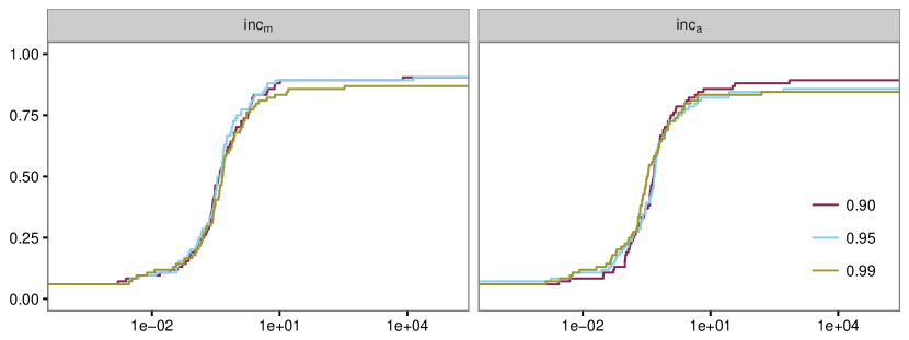
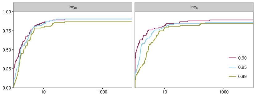
Figure 1. Non-dominated parameterizations $\lambda\in\left\{{0.9,0.95,0.99}\right\}$, $\operatorname{inc}\in\left\{{\operatorname{inc}_{\mathrm{m}},\operatorname{inc}_{\mathrm{a}}}\right\}$ (all with activated Gurobi presolve) for the penalty ADM based feasibility pump for MIPs. Top: primal-dual gap. Bottom: running times.

First, we present a parameter study. Our penalty ADM based feasibility pump can be instantiated using different choices for certain algorithmic parameters: The initial convex combination parameter $\alpha^{0}$ for weighting the objective function and the distance function $\tilde{\chi}$ (see Problem (18)) is always set to $\alpha^{0}=1$, emulating the objective feasibility pump of [1]. The parameter $\lambda$ for updating the convex combination parameter is varied in the set $\left\{{0.9,0.95,0.99}\right\}$ in our parameter study and the penalty parameter update operator can be chosen to be the additive variant $\operatorname{inc}_{\mathrm{a}}(x)=x+1$ or the multiplicative variant $\operatorname{inc}_{\mathrm{m}}(x)=10x$. In addition, we also tested the impact of (de)activating the MIP presolve of Gurobi before applying our method. Thus, combining the different choices for $\lambda,\operatorname{inc}$, and the (de)activation of Gurobi’s presolve leads to 12 parameter combinations. We applied every of these 12 variants of our method to solve the MIPLIB 2010 benchmark test set excluding the infeasible instances ash608gpia-3col, enlight14, and ns1766074. This yields a test set of 84 instances; see [35]. In order to determine the best parameterization, we compare all 12 variants using performance profiles, where the performance measure is chosen as defined in (19). We then exclude a parameterization $p$ if another parameterization $p^{\prime}$ exists that dominates $p$. Here, domination is defined by a performance profile completely left-above the other one. This yields the exclusion of deactivating Gurobi’s presolve and, thus, 6 remaining parameterizations; $\lambda\in\left\{{0.9,0.95,0.99}\right\}$ and $\operatorname{inc}\in\left\{{\operatorname{inc}_{\mathrm{m}},\operatorname{inc}_{\mathrm{a}}}\right\}$. The corresponding performance profiles are given in Figure 1.

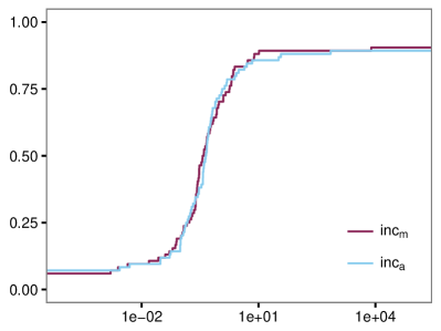
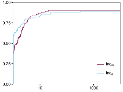
Figure 2. Performance profiles of primal-dual gap (left) and running times (right) for the winner parameterizations $\lambda=0.9$, activated Gurobi presolve, and $\operatorname{inc}\in\left\{{\operatorname{inc}_{\mathrm{m}},\operatorname{inc}_{\mathrm{a}}}\right\}$ for MIPs

It can be seen that lower values for $\lambda$ yield more robust instantiations of the algorithm, i.e., the number of instances for which a feasible solution can be found is larger. Additionally, all tested variants solve 5 out of 84 instances to global optimality, except for the variant with $\lambda=0.95$ and $\operatorname{inc}_{\text{a}}$ penalty parameter update rule, which solves 6 instances to global optimality. Altogether, the six parameter choices are quite comparable. Turning to running times, it can be clearly seen that smaller values of $\lambda$ also lead to shorter running times. Thus, our parameter study suggests to activate the MIP presolve of Gurobi, to choose $\lambda=$0.9$$, and to leave the choice of the penalty parameter update rule $\operatorname{inc}\in\left\{{\operatorname{inc}_{\mathrm{m}},\operatorname{inc}_{\mathrm{a}}}\right\}$ as an option for the user. Figure 2 shows the performance profiles for solution quality (left) and running times (right) for these “winning” parameterizations. We again see that some instances are solved to global optimality and that both parameterizations of our algorithm find a feasible solution for approximately $90\text{\,}\mathrm{\char 37\relax}$ of the MIPLIB 2010 benchmark instances (75 out of 84 instances for the $\operatorname{inc}_{\text{a}}$ update rule and 76 for the multiplicative rule $\operatorname{inc}_{\text{m}}$). Moreover, the multiplicative update operator $\operatorname{inc}_{\mathrm{m}}$ yields a slightly more robust algorithm, i.e., it finds a feasible solution for a few more instances than the additive version $\operatorname{inc}_{\mathrm{a}}$. The right part of Figure 2 compares the two winner instantiations w.r.t. running times. It can be seen that the additive $\operatorname{inc}_{\mathrm{a}}$ update operator tends to result in a faster algorithm for significantly more instances than the multiplicative version ($59.5\text{\,}\mathrm{\char 37\relax}$ vs. $38.1\text{\,}\mathrm{\char 37\relax}$).

Next, we compare our penalty ADM based feasibility pump with the objective feasibility pump of [1]. In order to achieve a fair comparison, we extend our method with a local branching strategy with an additional $k$-opt neighborhood constraint with $k=\min\left\{{20,\lfloor\mathchoice{\left\lvert I\right\rvert}{\lvert I\rvert}{\lvert I\rvert}{\lvert I\rvert}/10\rfloor}\right\}$ and a time limit $t^{+}-t^{*}$; see [25]. Here $t^{*}$ denotes the time spent in the penalty ADM based feasibility pump itself. Thus, the local branching stage serves as an improvement heuristic as it is also the case in [1].

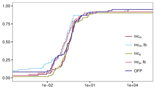
Figure 3. The two winner parameterizations (see Figure 2) with and without local branching compared to the objective feasibility pump (OFP) by [1]

As test instances we use all MIPLIB 2010 and MIPLIB 2003 instances that have been used in [1] as well. Figure 3 shows the primal-dual gap performance profiles of the two winner parameterizations ($\lambda=0.9$ and $\operatorname{inc}\in\left\{{\operatorname{inc}_{\mathrm{m}},\operatorname{inc}_{\mathrm{a}}}\right\}$) with and without local branching applied as an additional improvement heuristic as well as the corresponding performance profile curve based on the results reported by [1]. First of all, it can be seen that all five methods find a feasible solution for at least $90.2\text{\,}\mathrm{\char 37\relax}$ of the tested instances, which underpins the strength of feasibility pumps in general. Comparing only the different parameterization of our method we see that the $\operatorname{inc}_{\text{m}}$ update rule with local branching outperforms the version without local branching and both variants using the additive penalty update rule. The latter also performs similar independent of whether local branching is used or not, whereas the local branching stage significantly improves the solution quality when the $\operatorname{inc}_{\text{m}}$ rule is used (in which case we find a global optimal solution for $11.5\text{\,}\mathrm{\char 37\relax}$; compared to $8.2\text{\,}\mathrm{\char 37\relax}$ for the objective feasibility pump of [1]). One sees that the multiplicative update rule together with local branching slightly outperforms the objective feasibility pump of [1] w.r.t. solution quality.

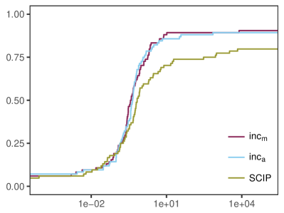
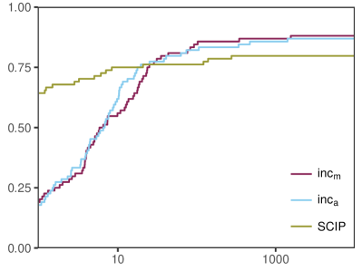
Figure 4. The two winner parameterizations (see Figure 2) with and without local branching compared to the feasibility pump implementation for MIPs of SCIP: primal dual gap (left) and running times (right)

We now turn to a comparison with the MIP solver SCIP 3.2.1. We used SCIP instead of, e.g., Cplex or Gurobi, for our comparison with a state-of-the-art MIP solver because SCIP is the only solver that allows to completely de-activate all other components of the solution process such that we can compare solution quality and running times. To this end, we de-activated SCIP’s presolve, all cuts, and all heuristics except for the feasibility pump. We also use a time limit of $1\text{\,}\mathrm{h}$, stop the algorithm after finding the first feasible solution, and use Cplex 12.6 as the internal LP solver. To be comparable with our feasibility pump implementation that uses Gurobi’s preprocessing, we presolved all 84 MIPLIB 2010 instances with Gurobi and solved these presolved instances with SCIP’s feasibility pump implementation. The results are given in Figure 4. The left figure shows the performance profile of the primal-dual gap. We see that we are again comparable in terms of solution quality and that our solutions tend to have a slightly better objective value. Moreover, we find a feasible solution for up to approximately $90\text{\,}\mathrm{\char 37\relax}$ of all instances, whereas SCIP finds a feasible point for slightly more than $75\text{\,}\mathrm{\char 37\relax}$. However, this comes at the price of significantly larger running times; see Figure 4 (right). SCIP is faster for almost all instances and solves most of them within approximately $10\text{\,}\mathrm{s}$. Although we did not try to tune our code extensively so far, the latter comparison shows that there is still a strong potential and a lot of work to do if our code should be competitive with a state-of-the-art heuristic w.r.t. running times.

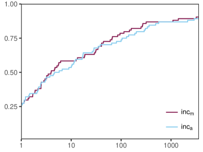
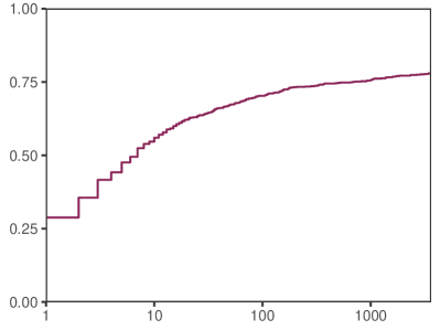
Figure 5. Left: Cumulative distribution function of absolute running times ($x$-axis; in s) for two winner parameterizations $\operatorname{inc}\in\left\{{\operatorname{inc}_{\mathrm{m}},\operatorname{inc}_{\mathrm{a}}}\right\}$ on all MIPLIB 2010 instances. Right: Cumulative distribution function of absolute running times ($x$-axis; in s) on all MINLPLib2 instances

In Figure 5 (left) cumulative distribution functions for absolute running times are given for both winner parameterizations of our algorithm for MIPs. It can be seen that for approximately $25\text{\,}\mathrm{\char 37\relax}$ of all instances a feasible solution is found in at most $1\text{\,}\mathrm{s}$ and $50\text{\,}\mathrm{\char 37\relax}60\text{\,}\mathrm{\char 37\relax}$ of all instances have been solved to feasibility within $10\text{\,}\mathrm{s}$. The geometric mean of the running times taken over all instances for which a feasible solution has been found within the time limit is $4.56\text{\,}\mathrm{s}$ for $\operatorname{inc}=\operatorname{inc}_{\mathrm{m}}$ and $4.94\text{\,}\mathrm{s}$ for $\operatorname{inc}=\operatorname{inc}_{\mathrm{a}}$. The running times for all instances can be found in Appendix A.

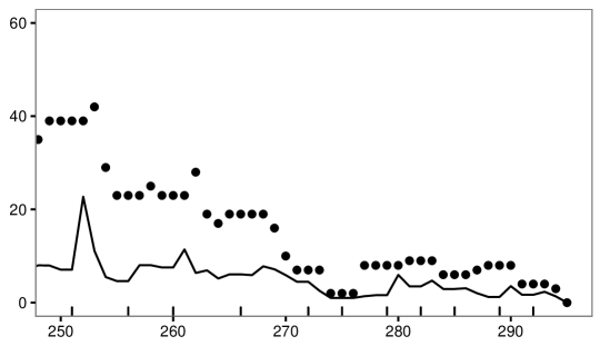
Figure 6. Number of fractional integer components (dots) and total fractionality (solid line) vs. ADM iterations. Penalty parameter updates are marked with small black vertical lines on top of the ADM iteration axis.

We close this section with an exemplary discussion of the course of integer (in)feasibility during the iterations of our method. Figure 6 shows the approximately 50 last iterations of our method applied to the MIPLIB 2010 instance rococoC10-001000. Dots correspond to numbers of fractional integer components and the solid line represents the course of the total fractionality measure

$$\sum_{i\in I}\mathchoice{\left\lvert x_{i}-\lfloor x_{i}+0.5\rfloor\right\rvert}{\lvert x_{i}-\lfloor x_{i}+0.5\rfloor\rvert}{\lvert x_{i}-\lfloor x_{i}+0.5\rfloor\rvert}{\lvert x_{i}-\lfloor x_{i}+0.5\rfloor\rvert}$$

of solutions $x$ of the continuous subproblems over the subsequent ADM iterations. The small black lines on top of the ADM iteration axis denote iterations at which the penalty parameters are updated.

First of all, we see that penalty parameter updates are applied whenever the ADM of the inner loop stalls, i.e., whenever the ADM of the inner loop entered an undesired integer infeasible partial minimum. The method stops after 295 ADM iterations with an integer feasible partial minimum. As expected, we typically see a sawtooth phenomenon: The total fractionality decreases between two consecutive penalty parameter updates and increases after a penalty parameter update. The number of fractional integer components follows this behavior qualitatively. The number of ADM iterations between two consecutive penalty parameter updates varies between 3 to 6 iterations. Thus, convergence to partial minima does not seem to be challenging for this specific instance.

5.2. Mixed-Integer Nonlinear Problems

We now turn to mixed-integer nonlinear programs. The penalty based ADM for this class of models has been implemented in C++ using the so-called GAMS Expert-level API with GAMS 24.5.4 [13]. The continuous relaxation models are solved with CONOPT 3.17A [21]. According to the results from Section 5.1 we choose the parameters $\alpha^{0}=1$ and $\lambda=0.9$. The penalty parameter update rule is chosen to be $\operatorname{inc}_{\mathrm{a}}(x)=x+1$ since this variant turned out to be favorable for MINLPs. We set the time limit to $1\text{\,}\mathrm{h}$ as for the MIP experiments and we do not incorporate any iteration limits for the inner ADM and the outer penalty loop. Throughout this section we declare an MINLP instance as solved to feasibility if CONOPT finds a feasible solution (w.r.t. its default tolerances) with all integer components fixed to integral values.

We compare the results of our method with other recently published numerical results concerning feasibility pump algorithms for convex and nonconvex MINLPs. Most of the results from the literature that we use for these comparisons are based on the first and second version of the MINLPLib; see [12]. Since a reasonable comparison of running times is not possible due to differences in the used hardware, we focus on the comparison of success rates and solution quality.

We also compared the obtained results separately for convex and nonconvex instances. As expected, the results of our method are slightly better for the convex case. However, the results are qualitatively rather similar and we thus present the following analysis of our computational results without distinguishing between convex and nonconvex instances.

First, we start with a comparison of different feasibility pump versions presented by [14] in [14] and our method on selected MINLPLib instances. [14] test their method on 65 MINLPLib instances. However, it turned out in the meantime that the used test set contained 4 duplicate instances. Thus, the following comparison is carried out on 61 MINLPLib instances. Figure 7 (left) displays the performance profiles using the primal-dual gap as the performance measure; see (19).

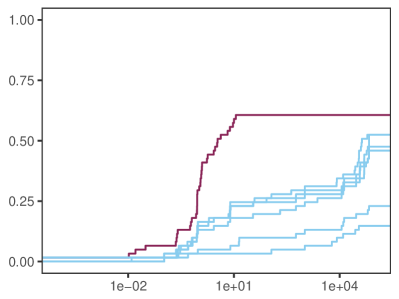
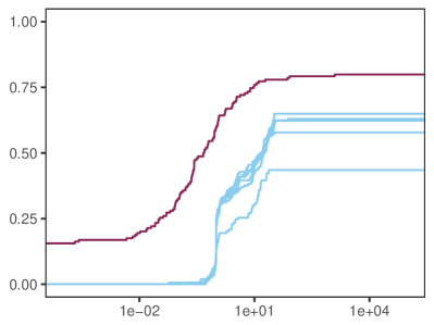
Figure 7. Left: Performance profiles for the primal-dual gap of the penalty ADM based feasibility pump (red) and all six feasibility pump variants (blue) for MINLPs presented in [14] on subset of 61 MINLPLib instances. Right: Performance profiles for the primal-dual gap of the penalty ADM based feasibility pump (red) and different feasibility pump variants (blue) proposed by [4]

It can be clearly seen that the penalty ADM based feasibility pump outperforms all feasibility pump variants presented in [14], although we used a time limit of $1\text{\,}\mathrm{h}$ in contrast to $2\text{\,}\mathrm{h}$ used in [14]. Although the number of instances solved to optimality is comparably low for all algorithms, the overall solution quality of our penalty ADM based algorithm is significantly higher than the quality of solutions obtained in [14]. Additionally, the number of instances for which we found a feasible solution is $60.7\text{\,}\mathrm{\char 37\relax}$ whereas the percentage of instances solved to feasibility in [14] ranges from $54.1\text{\,}\mathrm{\char 37\relax}$ to only $16.4\text{\,}\mathrm{\char 37\relax}$.

Complementing this comparison on the MINLPLib test set we also tested our method on 889 out of 1385 instances of the more recent MINLPLib2 test set. Here, we neglected all instances containing only continuous variables. Again, our method behaves quite satisfactory. It computes a feasible solution for 642 instances ($72.2\text{\,}\mathrm{\char 37\relax}$), leaving 247 instances unsolved. We compare our solutions with the dual bound given in the MINLPLib2. The penalty ADM based feasibility pump computes solutions with a vanishing primal-dual gap for 83 instances; i.e., for $9.3\text{\,}\mathrm{\char 37\relax}$ of all instances of the test set. The running times on all MINLPLib2 instances are given in the cumulative distribution function in Figure 5 (right). Remarkably, the results are quite comparable with those for the MIP instances: For approximately $50\text{\,}\mathrm{\char 37\relax}$ of all MINLPLib2 instances a feasible solution has been found within $10\text{\,}\mathrm{s}$ and slightly more than $25\text{\,}\mathrm{\char 37\relax}$ of the instances are solved to feasibility within $1\text{\,}\mathrm{s}$. The geometric mean of the running times taken over all instances for which a feasible solution has been found within the time limit is $5.36\text{\,}\mathrm{s}$. Nevertheless, the running times are fast enough so that the method could, in principle, be embedded in a global solver as a primal heuristic. As for the MIP results, a table with all running times and additional information is given in the appendix.

Finally, we discuss the most recent (at least to the best of our knowledge) results on a new variant of feasibility pumps for nonconvex mixed-integer nonlinear problems that are published by [4] in his PhD thesis [4]. The test set used by [4] is neither a sub- nor a superset of the current MINLPLib. Thus, we compare our method with the algorithms proposed by [4] on all instances of his test set that are also part of the current MINLPLib version, yielding a test set of 154 instances. Again, we compare the methods by performance profiles of the primal-dual gap, see Figure 7 (right). The penalty ADM based feasibility pump significantly outperforms all variants of the feasibility pump for MINLPs proposed by [4]. First, the methods of [4] do not solve any instance to optimality, whereas we close the primal-dual gap for $15.6\text{\,}\mathrm{\char 37\relax}$ of the instances. Second, our method finds a feasible solution for $79.9\text{\,}\mathrm{\char 37\relax}$ of the tested instances, whereas the methods of [4] solve approximately $43.5\text{\,}\mathrm{\char 37\relax}64.9\text{\,}\mathrm{\char 37\relax}$ to feasibility.

6. Summary

In this paper we have shown that idealized feasibility pumps, i.e., feasibility pumps without random perturbations, can be seen as alternating direction methods applied to a special reformulation of the original mixed-integer problem. This yields that idealized feasibility pumps converge to a partial minimum of the reformulated problem. If this partial minimum is not an integer feasible point, feasibility pumps apply a random perturbation to escape this undesired point. We replace this random restart with a penalty framework that encompasses the alternating direction method in the inner loop and that replaces random perturbations by tailored penalty parameter updates. This way it is possible for the first time to perform a theoretical study for a variant of the feasibility pump including restarts. The resulting penalty based alternating direction method can be applied to both MIPs and MINLPs. Our numerical results indicate that this new version of the feasibility pump is comparable (w.r.t. most recent publications) for the case of MIPs and clearly outperforms other feasibility pump algorithms on MINLPs in terms of solution quality.

Appendix A Detailed Results for the MIPLIB 2010

Table 1. Detailed numerical results for the penalty ADM based feasibility pump on all 84 feasible MIPLIB 2010 instances; see Section 5.1 Mixed-Integer Linear Problems. Objective function value, running times (s), outer penalty iterations (#Pen.), and inner ADM iterations (#ADM) for the method with $\lambda=0.9$, multiplicative penalty parameter update rule $\operatorname{inc}_{\text{m}}$, activated Gurobi presolve, and deactivated local branching.

Instance	Objective	Time	#Pen.	#ADM
30n20b8	906.00	40.42	892	3828
acc-tight5	—	—	—	—
aflow40b	3565.00	2.48	146	437
air04	71018.00	60.42	41	190
app1-2	-30.00	3189.86	4133	15567
bab5	-78587.20	34.25	178	540
beasleyC3	863.00	0.19	24	67
biella1	3743460.00	65.50	26	238
bienst2	73.25	0.21	20	76
binkar10_1	7263.57	0.23	32	112
bley_xl1	285.00	4.62	37	149
bnatt350	—	—	—	—
core2536-691	692.00	31.37	19	106
cov1075	120.00	0.17	12	24
csched010	—	—	—	—
danoint	78.00	1.70	24	101
dfn-gwin-UUM	125512.00	0.28	66	166
eil33-2	1373.60	0.74	19	64
eilB101	1513.00	0.94	17	66
enlight13	0.00	0.00	1	1
ex9	0.00	0.00	1	1
glass4	3390030000.00	0.28	103	353
gmu-35-40	-2159090.00	1.89	298	1073
iis-100-0-cov	100.00	0.27	12	24
iis-bupa-cov	100.00	2.16	12	38
iis-pima-cov	74.00	3.23	12	44
lectsched-4-obj	9.00	3.46	66	287
m100n500k4r1	-20.00	0.76	30	203
macrophage	522.00	0.32	14	30
map18	-280.00	250.17	120	317
map20	-371.00	159.76	127	306
mcsched	228737.00	1.37	13	56
mik-250-1-100-1	284980.00	0.48	71	202
mine-166-5	-22751900.00	1.16	22	54
mine-90-10	-558839000.00	1.69	58	173
msc98-ip	25797700.00	146.92	48	307
mspp16	407.00	1399.15	91	249
mzzv11	-16438.00	94.84	102	440
n3div36	170600.00	13.36	103	321
n3seq24	53600.00	271.77	71	315
n4-3	13980.00	0.28	13	35
neos-1109824	687.00	3.93	93	295
neos13	-28.04	5.54	23	91
neos-1337307	-201818.00	2.99	29	100
neos-1396125	—	—	—	—
neos-1601936	23409.00	266.56	66	629
neos18	17.00	0.87	21	86
neos-476283	407.01	66.98	78	226
neos-686190	16410.00	1.87	47	143
neos-849702	—	—	—	—
neos-916792	44.56	5.64	100	335
neos-934278	264.00	1091.80	57	225
net12	337.00	29.06	53	217
netdiversion	—	—	—	—
newdano	89.75	0.44	19	77
noswot	-38.00	0.17	61	240
ns1208400	—	—	—	—
ns1688347	35.00	6.14	49	227
ns1758913	-1454.67	18.37	5	15
ns1830653	—	—	—	—
opm2-z7-s2	-1519.00	35.30	13	37
pg5_34	-12628.50	0.76	65	195
pigeon-10	-9000.00	2.51	1091	2732
pw-myciel4	13.00	3.99	20	130
qiu	1235.01	0.44	19	51
rail507	183.00	30.66	35	158
ran16x16	4734.00	0.12	52	144
reblock67	-18739300.00	1.14	51	169
rmatr100-p10	494.00	2.49	12	41
rmatr100-p5	1327.00	5.18	11	39
rmine6	-239.11	3.21	32	93
rocII-4-11	-0.52	18.74	292	1162
rococoC10-001000	34598.00	1.43	68	295
roll3000	18404.00	2.83	48	207
satellites1-25	33.00	44.26	24	98
sp98ic	558066000.00	12.55	84	313
sp98ir	244287000.00	4.73	49	168
tanglegram1	6478.00	114.05	16	35
tanglegram2	1445.00	2.51	16	34
timtab1	1415540.00	0.27	41	153
triptim1	22.87	317.56	7	16
unitcal_7	20426600.00	40.69	112	400
vpphard	44.00	85.31	38	242
zib54-UUE	13164400.00	0.44	27	75

Appendix B Detailed Results for the MINLPLib2

Table 2. Detailed numerical results for the penalty ADM based feasibility pump on all 889 MINLPLib 2 instances with integer variables. Objective function value, running times (s), outer penalty iterations (#Pen.), and inner ADM iterations (#ADM) for the method with $\lambda=0.9$, additive penalty parameter update rule $\operatorname{inc}_{\text{a}}$, and deactivated local branching.

Instance	Objective	Time	#Pen.	#ADM
4stufen	118114.00	9	74	169
alan	3.00	0	5	7
autocorr_bern20-03	-64.00	0	1	1
autocorr_bern20-05	-396.00	2	1	1
autocorr_bern20-10	-2912.00	1	1	1
autocorr_bern20-15	-5936.00	1	1	1
autocorr_bern25-03	-80.00	0	1	1
autocorr_bern25-06	-936.00	0	3	4
autocorr_bern25-13	-7984.00	0	1	1
autocorr_bern25-19	-14472.00	0	1	1
autocorr_bern25-25	-10352.00	0	1	1
autocorr_bern30-04	-288.00	0	1	1
autocorr_bern30-08	-2912.00	0	1	1
autocorr_bern30-15	-15384.00	0	1	1
autocorr_bern30-23	-30240.00	1	1	1
autocorr_bern30-30	-22640.00	1	1	1
autocorr_bern35-04	-344.00	0	1	1
autocorr_bern35-09	-4976.00	0	1	1
autocorr_bern35-18	-30712.00	0	1	1
autocorr_bern35-26	-54960.00	0	1	1
autocorr_bern35-35	-40272.00	1	1	1
autocorr_bern40-05	-908.00	0	1	1
autocorr_bern40-10	-8192.00	0	1	1
autocorr_bern40-20	-50228.00	1	5	7
autocorr_bern40-30	-94040.00	1	1	1
autocorr_bern40-40	-66832.00	1	1	1
autocorr_bern45-05	-1004.00	0	3	4
autocorr_bern45-11	-12532.00	0	1	1
autocorr_bern45-23	-84844.00	0	1	1
autocorr_bern45-34	-151768.00	0	1	1
autocorr_bern45-45	-108528.00	1	1	1
autocorr_bern50-06	-2072.00	1	3	4
autocorr_bern50-13	-23176.00	0	1	1
autocorr_bern50-25	-123764.00	1	3	4
autocorr_bern50-38	-232808.00	0	1	1
autocorr_bern50-50	-166168.00	1	1	1
autocorr_bern55-06	-2288.00	0	3	4
autocorr_bern55-14	-32280.00	1	3	4
autocorr_bern55-28	-189404.00	0	1	1
autocorr_bern55-41	-335980.00	0	1	1
autocorr_bern55-55	-238296.00	1	1	1
autocorr_bern60-08	-6712.00	0	1	1
autocorr_bern60-15	-44368.00	0	1	1
autocorr_bern60-30	-258304.00	0	1	1
autocorr_bern60-45	-476456.00	1	1	1
autocorr_bern60-60	-347372.00	1	1	1
batch	309205.00	2	22	43
batch0812	2838520.00	5	64	107
batch0812_nc	3534900.00	4	32	70
batchdes	185769.00	0	7	13
batch_nc	363583.00	5	60	105
batchs101006m	776397.00	5	24	65
batchs121208m	1336450.00	7	22	73
batchs151208m	1588930.00	12	37	120
batchs201210m	2408440.00	17	72	157
bchoco05	0.95	1	3	4
bchoco06	0.96	0	3	4
bchoco07	0.96	2	3	4
bchoco08	—	—	—	—
beuster	128512.00	15	99	254
blend029	—	—	68919	68961
blend146	29.93	8	76	110
blend480	-8.24	56	655	753
blend531	—	—	53222	53555
blend718	1.23	6	30	77
blend721	-0.87	4	27	56
blend852	46.13	9	87	126
blendgap	-0.00	0	1	1
cardqp_inlp	3843.61	0	1	1
cardqp_iqp	3843.61	0	1	1
carton7	303.88	368	4645	5010
carton9	340.75	15	77	155
casctanks	9.16	3	40	46
case_1scv2	7791.24	16	33	86
cecil_13	-115564.00	9	65	92
chp_partload	—	—	25492	25701
clay0203h	41709.80	81	1498	1519
clay0203m	41737.50	50	1002	1022
clay0204h	7830.00	5	50	82
clay0204m	10340.00	3	35	48
clay0205h	23484.20	43	609	715
clay0205m	9715.00	5	57	86
clay0303h	36613.00	56	954	996
clay0303m	41737.50	8	101	170
clay0304h	61315.90	52	764	859
clay0304m	61831.50	38	694	748
clay0305h	43405.70	10	132	161
clay0305m	24593.10	7	92	121
contvar	829318.00	7	8	35
crossdock_15x7	14467.00	6	62	99
crossdock_15x8	16765.00	1856	26313	27298
crudeoil_lee1_05	79.35	75	808	851
crudeoil_lee1_06	78.75	70	555	655
crudeoil_lee1_07	78.75	2868	24641	25051
crudeoil_lee1_08	79.35	18	72	106
crudeoil_lee1_09	78.75	918	5556	5841
crudeoil_lee1_10	78.75	32	103	153
crudeoil_lee2_05	90.00	31	117	158
crudeoil_lee2_06	97.59	114	265	401
crudeoil_lee2_07	90.00	329	949	1114
crudeoil_lee2_08	—	—	12801	13253
crudeoil_lee2_09	—	—	—	—
crudeoil_lee2_10	—	—	7412	8007
crudeoil_lee3_05	82.00	173	996	1033
crudeoil_lee3_06	84.49	125	574	606
crudeoil_lee3_07	82.90	29	35	65
crudeoil_lee3_08	—	—	13112	13645
crudeoil_lee3_09	82.75	66	85	108
crudeoil_lee3_10	77.50	144	145	198
crudeoil_lee4_05	132.48	13	15	21
crudeoil_lee4_06	132.49	16	15	22
crudeoil_lee4_07	132.55	170	272	333
crudeoil_lee4_08	131.54	175	192	299
crudeoil_lee4_09	—	—	5326	5417
crudeoil_lee4_10	—	—	4329	4802
crudeoil_li01	4852.37	1247	19259	19368
crudeoil_li02	—	—	—	—
crudeoil_li03	—	—	31637	32220
crudeoil_li05	3030.59	34	225	312
crudeoil_li06	3303.84	111	869	947
crudeoil_li11	—	—	26706	27063
crudeoil_li21	—	—	19307	19619
csched1	-30174.60	0	4	5
csched1a	-29903.30	1	7	13
csched2	-160668.00	2	9	20
csched2a	-162047.00	7	44	120
deb10	209.43	1	9	13
deb6	251.66	1	3	4
deb7	176.08	2	3	4
deb8	176.08	1	3	4
deb9	176.08	1	3	4
densitymod	—	—	4	8
dosemin2d	173.98	11	5	11
dosemin3d	1.32	29	7	13
du-opt	5.34	0	3	4
du-opt5	112.02	0	5	8
edgecross10-010	4.00	0	1	1
edgecross10-020	19.00	0	1	1
edgecross10-030	53.00	0	3	4
edgecross10-040	142.00	0	3	4
edgecross10-050	301.00	1	1	1
edgecross10-060	470.00	0	1	1
edgecross10-070	735.00	0	1	1
edgecross10-080	1048.00	0	1	1
edgecross10-090	1387.00	0	1	1
edgecross14-019	5.00	0	1	1
edgecross14-039	123.00	1	1	1
edgecross14-058	391.00	0	1	1
edgecross14-078	725.00	0	1	1
edgecross14-098	1392.00	0	1	1
edgecross14-117	2168.00	1	3	4
edgecross14-137	2880.00	0	1	1
edgecross14-156	4342.00	0	3	4
edgecross14-176	5956.00	1	1	1
edgecross20-040	73.00	1	1	1
edgecross20-080	530.00	1	1	1
edgecross22-048	97.00	2	1	1
edgecross22-096	980.00	4	3	4
edgecross24-057	213.00	3	1	1
edgecross24-115	1429.00	3	1	1
eg_all_s	8.67	11	20	44
eg_disc2_s	5.68	3	3	4
eg_disc_s	6.03	6	7	15
eg_int_s	8.32	7	6	13
elf	1.68	1	1	1
eniplac	-120713.00	43	636	764
enpro48pb	188887.00	1	10	23
enpro56pb	266762.00	3	24	56
ethanolh	-157.59	0	4	5
ethanolm	-31.27	9	116	168
ex1221	7.67	0	1	1
ex1222	1.08	0	6	10
ex1223	5.81	1	6	10
ex1223a	5.81	1	5	8
ex1223b	5.81	1	6	10
ex1224	-0.88	1	12	19
ex1225	31.00	0	6	9
ex1226	-17.00	0	1	1
ex1233	201540.00	3	21	49
ex1243	135552.00	2	18	47
ex1244	95046.40	1	13	17
ex1252	—	—	—	—
ex1252a	143555.00	3	23	54
ex1263	69.60	86	1665	1773
ex1263a	38.60	55	1101	1142
ex1264	31.60	11	185	222
ex1264a	10.00	5	90	108
ex1265	22.30	16	231	343
ex1265a	15.10	4	60	87
ex1266	—	—	62770	64607
ex1266a	16.30	1	7	13
ex3pb	103.58	2	19	37
ex4	659.57	4	46	77
fac1	172954000.00	9	85	185
fac2	407585000.00	5	35	97
fac3	34789500.00	3	23	53
faclay20h	16941.00	0	1	1
faclay25	5107.00	1	1	1
faclay30	8970.00	3	1	1
faclay30h	50775.00	3	1	1
faclay33	67677.00	6	1	1
faclay35	77040.00	8	1	1
faclay60	1564130.00	15	1	1
faclay70	1656440.00	2316	1	1
faclay75	—	—	1	0
faclay80	—	—	1	0
feedtray	-13.41	1	1	1
feedtray2	—	—	—	—
fin2bb	0.00	2	19	26
flay02h	37.95	2	20	40
flay02m	37.95	2	24	45
flay03h	48.99	4	26	60
flay03m	48.99	3	29	61
flay04h	54.99	6	50	100
flay04m	54.99	4	42	85
flay05h	80.99	7	36	97
flay05m	64.50	5	41	96
flay06h	106.88	11	38	121
flay06m	66.93	6	43	102
fo7	25.60	87	1643	1691
fo7_2	40.43	15	171	236
fo7_ar2_1	55.38	317	5449	5627
fo7_ar25_1	—	—	65860	66079
fo7_ar3_1	34.49	13	97	212
fo7_ar4_1	41.66	1369	25281	25479
fo7_ar5_1	38.09	7	53	110
fo8	47.40	7	66	99
fo8_ar2_1	—	—	62624	62999
fo8_ar25_1	—	—	61119	61451
fo8_ar3_1	45.34	38	469	590
fo8_ar4_1	38.66	36	384	529
fo8_ar5_1	51.84	370	5769	5963
fo9	52.78	7	60	109
fo9_ar2_1	—	—	52908	53324
fo9_ar25_1	—	—	57149	57561
fo9_ar3_1	49.40	46	446	592
fo9_ar4_1	—	—	54254	54687
fo9_ar5_1	51.17	11	72	131
fuel	8566.12	2	16	42
fuzzy	—	—	1	10135
gams01	26878.30	36	100	261
gams02	99281400.00	3427	7309	8005
gams03	—	—	10477	10747
gasnet	6999380.00	10	97	194
gasprod_sarawak01	-31599.40	1	5	7
gasprod_sarawak16	-31399.40	5	11	16
gasprod_sarawak81	-31399.40	60	11	16
gastrans	—	—	71678	71681
gastrans040	0.00	1	3	4
gastrans135	0.00	63	517	524
gastrans582_cold13	—	—	24865	24973
gastrans582_cold13_95	—	—	26008	26017
gastrans582_cold17	0.00	12	34	40
gastrans582_cold17_95	0.00	13	38	45
gastrans582_cool12	0.00	10	22	27
gastrans582_cool12_95	—	—	25893	25904
gastrans582_cool14	—	—	6717	20655
gastrans582_cool14_95	—	—	24012	24195
gastrans582_freezing27	—	—	21961	22878
gastrans582_freezing27_95	—	—	649	19415
gastrans582_freezing30	—	—	25209	25221
gastrans582_freezing30_95	0.00	108	728	736
gastrans582_mild10	—	—	23990	23997
gastrans582_mild10_95	—	—	25798	25810
gastrans582_mild11	0.00	49	295	304
gastrans582_mild11_95	—	—	25515	25527
gastrans582_warm15	—	—	24775	25032
gastrans582_warm15_95	—	—	24674	24934
gastrans582_warm31	0.00	44	271	279
gastrans582_warm31_95	—	—	26392	26403
gbd	2.20	0	1	1
gear	0.00	1	3	4
gear2	0.01	0	4	6
gear3	0.00	1	3	4
gear4	120.67	5	70	87
genpooling_lee1	—	—	—	—
genpooling_lee2	—	—	—	—
genpooling_meyer04	—	—	—	—
genpooling_meyer10	—	—	—	—
genpooling_meyer15	—	—	—	—
ghg_1veh	7.78	0	1	1
ghg_2veh	7.78	0	1	1
ghg_3veh	7.77	0	4	5
gkocis	-1.41	1	7	9
graphpart_2g-0044-1601	-789955.00	1	1	1
graphpart_2g-0055-0062	—	—	68626	68626
graphpart_2g-0066-0066	-2082170.00	11	110	215
graphpart_2g-0077-0077	—	—	66436	66436
graphpart_2g-0088-0088	-5701630.00	0	1	1
graphpart_2g-0099-9211	-4495840.00	0	4	5
graphpart_2g-1010-0824	-6583360.00	0	1	1
graphpart_2pm-0044-0044	-11.00	0	1	1
graphpart_2pm-0055-0055	—	—	70312	70312
graphpart_2pm-0066-0066	-27.00	1	6	9
graphpart_2pm-0077-0777	—	—	64537	64537
graphpart_2pm-0088-0888	-46.00	0	4	5
graphpart_2pm-0099-0999	-56.00	1	18	22
graphpart_3g-0234-0234	—	—	69513	69513
graphpart_3g-0244-0244	-2702200.00	0	1	1
graphpart_3g-0333-0333	—	—	66677	66677
graphpart_3g-0334-0334	-3279970.00	0	1	1
graphpart_3g-0344-0344	—	—	66770	66770
graphpart_3g-0444-0444	-6621100.00	0	1	1
graphpart_3pm-0234-0234	—	—	74786	74786
graphpart_3pm-0244-0244	-27.00	0	1	1
graphpart_3pm-0333-0333	—	—	71653	71653
graphpart_3pm-0334-0334	-33.00	0	1	1
graphpart_3pm-0344-0344	—	—	68708	68708
graphpart_3pm-0444-0444	-57.00	1	4	5
graphpart_clique-20	147.00	0	1	1
graphpart_clique-30	495.00	0	1	1
graphpart_clique-40	1183.00	0	1	1
graphpart_clique-50	—	—	60889	60889
graphpart_clique-60	4010.00	2	34	36
graphpart_clique-70	—	—	50784	50784
hda	-4322.55	6	18	39
heatexch_gen1	410804.00	2	19	42
heatexch_gen2	739019.00	1	20	26
heatexch_gen3	109097.00	4	28	46
heatexch_spec1	219858.00	2	18	42
heatexch_spec2	849922.00	0	3	4
heatexch_spec3	319465.00	1	8	13
heatexch_trigen	977262.00	144	2367	2602
hmittelman	16.00	2	22	39
hybriddynamic_fixed	1.47	0	7	12
hybriddynamic_var	1.54	0	5	9
hydroenergy1	207178.00	2	29	39
hydroenergy2	369251.00	4	31	42
hydroenergy3	742404.00	7	31	44
ibs2	4.88	1032	55	125
jit1	173983.00	0	3	4
johnall	-222.37	5	54	57
kport20	33.50	2	14	37
kport40	42.02	70	1184	1289
lip	5428650.00	0	3	6
lop97ic	4535.18	7	10	31
lop97icx	4590.48	3	13	31
m3	55.80	2	21	32
m6	123.98	13	105	206
m7	—	—	66377	66664
m7_ar2_1	—	—	65520	65796
m7_ar25_1	—	—	69125	69424
m7_ar3_1	—	—	66925	67206
m7_ar4_1	450.97	127	1993	2166
m7_ar5_1	511.21	61	857	1025
mbtd	5.58	66	13	41
meanvarx	14.37	1	23	26
meanvarxsc	—	—	—	—
milinfract	2.63	8	5	7
minlphix	345.51	3	53	63
multiplants_mtg1a	363.57	2	17	35
multiplants_mtg1b	212.21	33	602	617
multiplants_mtg1c	406.98	5	31	52
multiplants_mtg2	7051.41	4	65	75
multiplants_mtg5	4706.88	75	1228	1258
multiplants_mtg6	4032.27	13	155	177
multiplants_stg1	250.44	1000	16363	16375
multiplants_stg1a	38.85	19	267	284
multiplants_stg1b	136.38	35	498	506
multiplants_stg1c	—	—	61799	61808
multiplants_stg5	—	—	52743	52952
multiplants_stg6	—	—	45323	46702
ndcc12	108.11	8	59	106
ndcc12persp	—	—	—	—
ndcc13	94.17	6	17	56
ndcc13persp	—	—	—	—
ndcc14	130.16	19	70	247
ndcc14persp	—	—	—	—
ndcc15	95.28	4	22	50
ndcc15persp	—	—	—	—
ndcc16	131.63	7	28	67
ndcc16persp	—	—	—	—
netmod_dol1	-0.01	18	22	40
netmod_dol2	-0.49	37	16	44
netmod_kar1	0.00	3	17	31
netmod_kar2	0.00	3	17	31
no7_ar2_1	—	—	66159	66423
no7_ar25_1	175.87	156	2635	2871
no7_ar3_1	149.22	13	142	201
no7_ar4_1	188.94	141	2040	2246
no7_ar5_1	153.84	148	2440	2576
nous1	1.57	0	3	4
nous2	0.63	0	3	4
nuclear104	—	—	—	—
nuclear10a	—	—	1737	2056
nuclear10b	-1.15	1604	31	124
nuclear14	-1.13	3	4	5
nuclear14a	-1.13	1	1	1
nuclear14b	-1.09	13	51	73
nuclear25	-1.12	7	22	29
nuclear25a	-1.12	5	22	29
nuclear25b	-1.09	29	63	153
nuclear49	-1.15	30	13	17
nuclear49a	-1.15	26	25	33
nuclear49b	-1.13	133	25	74
nuclearva	-1.01	3	33	45
nuclearvb	-1.02	1	1	1
nuclearvc	-0.98	5	49	59
nuclearvd	-1.04	10	63	75
nuclearve	-1.02	1	7	9
nuclearvf	—	—	—	—
nvs01	13.10	1	5	7
nvs02	5.96	2	35	38
nvs03	16.00	0	11	14
nvs04	—	—	—	—
nvs05	5.47	0	3	4
nvs06	1.86	1	3	4
nvs07	4.00	1	5	6
nvs08	23.83	1	10	14
nvs09	-43.13	0	1	1
nvs10	-308.40	0	4	7
nvs11	-416.40	3	69	74
nvs12	-477.00	0	3	5
nvs13	-585.20	1	3	5
nvs14	-40358.20	2	35	38
nvs15	1.00	0	3	4
nvs16	14.20	7	55	108
nvs17	-1078.20	3	52	57
nvs18	-778.40	0	3	5
nvs19	-1070.00	1	10	17
nvs20	230.92	1	7	13
nvs21	-4.27	8	172	174
nvs22	6.06	0	4	6
nvs23	-1078.40	1	3	5
nvs24	-1001.00	1	7	14
o7	190.62	25	374	418
o7_2	161.38	17	147	281
o7_ar2_1	—	—	61789	62056
o7_ar25_1	160.47	173	2936	3100
o7_ar3_1	162.83	34	446	562
o7_ar4_1	182.29	69	971	1138
o7_ar5_1	166.99	85	1274	1443
o8_ar4_1	345.47	22	130	256
o9_ar4_1	341.57	55	497	691
oaer	-1.92	1	4	5
oil	-0.87	2	3	4
oil2	-0.73	1	3	4
ortez	-9532.04	2	13	20
parallel	—	—	65520	65520
pb302035	4052260.00	28	25	34
pb302055	4087020.00	152	155	200
pb302075	4624370.00	62	49	77
pb302095	—	—	3207	4701
pb351535	5474850.00	180	240	306
pb351555	5256790.00	26	21	41
pb351575	6457260.00	16	15	21
pb351595	11847500.00	915	919	1524
pooling_epa1	-280.81	8	110	134
pooling_epa2	-4268.72	3	36	44
pooling_epa3	—	—	—	—
portfol_buyin	0.04	1	3	4
portfol_card	0.03	1	5	8
portfol_classical050_1	-0.09	1	10	21
portfol_classical200_2	-0.06	8	18	50
portfol_robust050_34	-0.00	1	11	16
portfol_robust100_09	-0.08	2	11	23
portfol_robust200_03	-0.08	12	16	44
portfol_roundlot	0.15	3412	5488	69538
portfol_shortfall050_68	-1.06	1	10	15
portfol_shortfall100_04	-1.07	3	13	25
portfol_shortfall200_05	-1.06	7	14	27
primary	—	—	—	—
prob02	112235.00	1	10	13
prob03	11.00	2	18	31
prob10	3.45	0	3	4
procsel	-1.41	0	5	7
product	-2075.33	16	56	103
product2	—	—	—	—
qap	411560.00	6	13	28
qapw	395664.00	48	106	345
ravempb	269590.00	1	10	23
risk2bpb	-55.48	1	17	21
routingdelay_bigm	—	—	27714	27777
routingdelay_proj	149.70	25	145	170
rsyn0805h	1280.01	1	17	26
rsyn0805m	928.36	3	24	50
rsyn0805m02h	2121.61	5	9	24
rsyn0805m02m	923.55	6	34	80
rsyn0805m03h	2996.90	7	8	19
rsyn0805m03m	2256.38	8	33	77
rsyn0805m04h	7145.11	7	5	11
rsyn0805m04m	4641.20	10	32	78
rsyn0810h	1675.12	2	18	26
rsyn0810m	801.54	3	21	49
rsyn0810m02h	1631.39	5	9	24
rsyn0810m02m	987.64	6	32	76
rsyn0810m03h	2671.49	8	7	18
rsyn0810m03m	2355.46	20	162	226
rsyn0810m04h	6472.92	23	12	26
rsyn0810m04m	4525.62	11	25	71
rsyn0815h	1262.05	1	11	21
rsyn0815m	923.47	3	26	52
rsyn0815m02h	1579.85	6	11	30
rsyn0815m02m	598.63	6	32	71
rsyn0815m03h	2702.87	10	8	20
rsyn0815m03m	2697.07	10	35	81
rsyn0815m04h	3220.26	21	9	24
rsyn0815m04m	1329.02	13	30	79
rsyn0820h	1138.41	2	9	17
rsyn0820m	723.84	4	24	56
rsyn0820m02h	1005.44	6	8	18
rsyn0820m02m	258.97	7	32	84
rsyn0820m03h	1984.43	14	8	16
rsyn0820m03m	1800.99	17	52	113
rsyn0820m04h	2363.62	25	8	23
rsyn0820m04m	1642.15	18	30	89
rsyn0830h	506.70	2	10	19
rsyn0830m	203.31	4	30	64
rsyn0830m02h	661.04	4	8	18
rsyn0830m02m	-273.98	6	33	68
rsyn0830m03h	1431.22	10	8	18
rsyn0830m03m	137.73	12	34	85
rsyn0830m04h	2284.01	21	9	19
rsyn0830m04m	128.87	19	36	90
rsyn0840h	297.64	2	6	14
rsyn0840m	54.73	5	30	69
rsyn0840m02h	612.11	5	10	18
rsyn0840m02m	-362.91	7	29	70
rsyn0840m03h	2664.97	15	11	20
rsyn0840m03m	2121.79	12	30	72
rsyn0840m04h	2327.32	21	8	16
rsyn0840m04m	-18.45	21	32	84
saa_2	12.75	35	50	78
sep1	-510.08	0	5	7
sepasequ_complex	538.16	12	55	97
sepasequ_convent	514.98	11	24	34
sfacloc1_2_80	13.55	1	3	4
sfacloc1_2_90	29.57	0	3	4
sfacloc1_2_95	18.85	0	1	1
sfacloc1_3_80	9.10	0	3	4
sfacloc1_3_90	11.88	0	3	4
sfacloc1_3_95	12.46	0	1	1
sfacloc1_4_80	8.46	1	3	4
sfacloc1_4_90	12.00	0	3	4
sfacloc1_4_95	11.24	1	3	4
sfacloc2_2_80	—	—	38561	38572
sfacloc2_2_90	29.96	7	77	109
sfacloc2_2_95	30.30	92	1745	1788
sfacloc2_3_80	25.20	15	82	127
sfacloc2_3_90	29.73	9	103	143
sfacloc2_3_95	25.17	3	27	54
sfacloc2_4_80	21.03	156	1403	1510
sfacloc2_4_90	28.72	87	1272	1390
sfacloc2_4_95	26.74	682	11503	11784
slay04h	14763.90	3	20	44
slay04m	12200.30	1	20	37
slay05h	24164.50	3	16	38
slay05m	23290.00	1	14	28
slay06h	38850.80	3	19	46
slay06m	33168.50	2	16	35
slay07h	69708.50	5	26	58
slay07m	70870.80	3	27	60
slay08h	105595.00	7	28	71
slay08m	85921.30	3	25	52
slay09h	156117.00	10	30	83
slay09m	160234.00	5	31	86
slay10h	197463.00	18	37	106
slay10m	176821.00	4	29	73
smallinvDAXr1b010-011	—	—	—	—
smallinvDAXr1b020-022	—	—	—	—
smallinvDAXr1b050-055	—	—	—	—
smallinvDAXr1b100-110	—	—	—	—
smallinvDAXr1b150-165	—	—	—	—
smallinvDAXr1b200-220	—	—	—	—
smallinvDAXr2b010-011	—	—	—	—
smallinvDAXr2b020-022	—	—	—	—
smallinvDAXr2b050-055	—	—	—	—
smallinvDAXr2b100-110	—	—	—	—
smallinvDAXr2b150-165	—	—	—	—
smallinvDAXr2b200-220	—	—	—	—
smallinvDAXr3b010-011	—	—	—	—
smallinvDAXr3b020-022	—	—	—	—
smallinvDAXr3b050-055	—	—	—	—
smallinvDAXr3b100-110	—	—	—	—
smallinvDAXr3b150-165	—	—	—	—
smallinvDAXr3b200-220	—	—	—	—
smallinvDAXr4b010-011	—	—	—	—
smallinvDAXr4b020-022	—	—	—	—
smallinvDAXr4b050-055	—	—	—	—
smallinvDAXr4b100-110	—	—	—	—
smallinvDAXr4b150-165	—	—	—	—
smallinvDAXr4b200-220	—	—	—	—
smallinvDAXr5b010-011	—	—	—	—
smallinvDAXr5b020-022	—	—	—	—
smallinvDAXr5b050-055	—	—	—	—
smallinvDAXr5b100-110	—	—	—	—
smallinvDAXr5b150-165	—	—	—	—
smallinvDAXr5b200-220	—	—	—	—
smallinvSNPr1b010-011	—	—	—	—
smallinvSNPr1b020-022	—	—	—	—
smallinvSNPr1b050-055	—	—	—	—
smallinvSNPr1b100-110	—	—	—	—
smallinvSNPr1b150-165	—	—	—	—
smallinvSNPr1b200-220	—	—	—	—
smallinvSNPr2b010-011	—	—	—	—
smallinvSNPr2b020-022	—	—	—	—
smallinvSNPr2b050-055	—	—	—	—
smallinvSNPr2b100-110	—	—	—	—
smallinvSNPr2b150-165	—	—	—	—
smallinvSNPr2b200-220	—	—	—	—
smallinvSNPr3b010-011	—	—	—	—
smallinvSNPr3b020-022	—	—	—	—
smallinvSNPr3b050-055	—	—	—	—
smallinvSNPr3b100-110	—	—	—	—
smallinvSNPr3b150-165	—	—	—	—
smallinvSNPr3b200-220	—	—	—	—
smallinvSNPr4b010-011	—	—	—	—
smallinvSNPr4b020-022	—	—	—	—
smallinvSNPr4b050-055	—	—	—	—
smallinvSNPr4b100-110	—	—	—	—
smallinvSNPr4b150-165	—	—	—	—
smallinvSNPr4b200-220	—	—	—	—
smallinvSNPr5b010-011	—	—	—	—
smallinvSNPr5b020-022	—	—	—	—
smallinvSNPr5b050-055	—	—	—	—
smallinvSNPr5b100-110	—	—	—	—
smallinvSNPr5b150-165	—	—	—	—
smallinvSNPr5b200-220	—	—	—	—
space25	919.99	279	3235	4234
space25a	657.73	5	80	106
space960	7985000.00	106	39	111
spectra2	14.04	3	25	53
sporttournament06	10.00	0	3	4
sporttournament08	22.00	0	1	1
sporttournament10	38.00	0	1	1
sporttournament12	58.00	0	1	1
sporttournament14	80.00	0	1	1
sporttournament16	100.00	0	3	4
sporttournament18	134.00	0	1	1
sporttournament20	162.00	1	3	4
sporttournament22	198.00	0	3	4
sporttournament24	230.00	0	1	1
sporttournament26	282.00	0	1	1
sporttournament28	298.00	0	3	4
sporttournament30	318.00	0	1	1
sporttournament32	384.00	0	1	1
sporttournament34	438.00	1	1	1
sporttournament36	472.00	0	1	1
sporttournament38	526.00	0	1	1
sporttournament40	590.00	0	1	1
sporttournament42	666.00	0	1	1
sporttournament44	706.00	0	1	1
sporttournament46	806.00	0	1	1
sporttournament48	904.00	0	1	1
sporttournament50	948.00	1	1	1
spring	1.35	1	19	27
squfl010-025	233.69	3	20	41
squfl010-025persp	214.11	247	3	776
squfl010-040	283.98	5	21	43
squfl010-040persp	240.60	72	1	100
squfl010-080	523.50	8	22	45
squfl010-080persp	509.70	1418	4	1684
squfl015-060	422.51	5	24	49
squfl015-060persp	366.62	522	8	367
squfl015-080	596.93	10	29	56
squfl015-080persp	407.13	994	3	608
squfl020-040	286.55	4	23	45
squfl020-040persp	221.02	339	11	249
squfl020-050	323.25	7	25	50
squfl020-050persp	244.05	331	11	193
squfl020-150	1131.79	113	36	73
squfl020-150persp	562.07	2348	15	384
squfl025-025	244.44	4	22	43
squfl025-025persp	178.63	719	10	645
squfl025-030	215.34	3	19	37
squfl025-030persp	215.34	1367	10	1057
squfl025-040	299.01	7	24	47
squfl025-040persp	225.39	650	29	385
squfl030-100	766.47	36	33	66
squfl030-100persp	—	—	3	535
squfl030-150	628.11	374	31	61
squfl030-150persp	—	—	10	307
squfl040-080	294.95	50	22	43
squfl040-080persp	578.72	2651	23	378
sssd08-04	203796.00	2	12	36
sssd08-04persp	413575.00	2	18	38
sssd12-05	421690.00	3	18	51
sssd12-05persp	458644.00	2	21	52
sssd15-04	266257.00	1	14	37
sssd15-04persp	281947.00	3	21	47
sssd15-06	782066.00	4	21	61
sssd15-06persp	553100.00	2	12	28
sssd15-08	882079.00	5	26	77
sssd15-08persp	599059.00	3	17	49
sssd16-07	666186.00	4	25	78
sssd16-07persp	421588.00	2	14	29
sssd18-06	438633.00	3	14	41
sssd18-06persp	484779.00	2	18	47
sssd18-08	949385.00	5	46	100
sssd18-08persp	1054060.00	4	21	67
sssd20-04	402023.00	7	16	42
sssd20-04persp	403765.00	3	20	58
sssd20-08	522836.00	3	14	59
sssd20-08persp	568422.00	3	21	55
sssd22-08	600312.00	5	22	59
sssd22-08persp	567598.00	3	22	59
sssd25-04	302373.00	2	19	46
sssd25-04persp	300946.00	2	30	55
sssd25-08	585480.00	3	19	55
sssd25-08persp	601061.00	3	20	51
st_e13	—	—	—	—
st_e14	5.81	0	6	10
st_e15	—	—	—	—
st_e27	2.00	0	1	1
st_e29	-0.88	1	12	19
st_e31	—	—	—	—
st_e32	-0.72	14	243	289
st_e35	71468.10	1	3	4
st_e36	—	—	8225	51928
st_e38	7197.73	0	1	1
st_e40	—	—	—	—
st_miqp1	380.50	1	15	28
st_miqp2	2.00	1	12	16
st_miqp3	—	—	—	—
st_miqp4	—	—	—	—
st_miqp5	-333.89	0	1	1
stockcycle	260786.00	12	147	218
st_test1	0.00	1	6	11
st_test2	—	—	—	—
st_test3	—	—	—	—
st_test4	—	—	—	—
st_test5	-110.00	2	28	46
st_test6	664.00	3	46	75
st_test8	-29605.00	0	4	5
st_testgr1	-12.76	1	11	15
st_testgr3	-20.50	2	19	29
st_testph4	-80.50	0	3	5
super1	—	—	—	—
super2	—	—	—	—
super3	—	—	—	—
super3t	—	—	—	—
supplychain	—	—	—	—
supplychainp1_020306	593975.00	0	3	5
supplychainp1_022020	3378850.00	5	5	9
supplychainp1_030510	1215690.00	0	3	5
supplychainp1_053050	8543940.00	111	5	11
supplychainr1_020306	628623.00	0	5	9
supplychainr1_022020	4050140.00	8	14	43
supplychainr1_030510	1568450.00	1	10	16
supplychainr1_053050	8588080.00	180	32	122
syn05h	837.73	0	3	4
syn05m	831.45	1	10	18
syn05m02h	3032.74	0	3	4
syn05m02m	3026.74	1	13	25
syn05m03h	4027.37	0	3	4
syn05m03m	3987.03	1	10	22
syn05m04h	5510.39	0	3	4
syn05m04m	5499.39	1	13	28
syn10h	1267.35	0	3	4
syn10m	560.25	0	10	14
syn10m02h	2310.30	1	3	4
syn10m02m	2275.85	2	13	25
syn10m03h	3354.68	1	3	4
syn10m03m	2773.64	2	25	38
syn10m04h	4557.06	0	3	4
syn10m04m	3814.77	3	26	41
syn15h	853.28	0	3	4
syn15m	503.63	1	10	25
syn15m02h	2832.75	0	3	4
syn15m02m	2777.75	1	14	25
syn15m03h	3850.18	0	3	4
syn15m03m	3795.18	3	17	34
syn15m04h	4937.48	1	3	4
syn15m04m	4882.48	2	18	31
syn20h	924.26	1	3	4
syn20m	722.64	2	8	19
syn20m02h	1752.13	1	3	4
syn20m02m	1693.13	2	23	38
syn20m03h	2646.95	1	3	4
syn20m03m	2574.01	3	18	41
syn20m04h	3532.74	1	3	4
syn20m04m	3475.74	3	18	35
syn30h	134.03	0	3	5
syn30m	-38.75	2	15	28
syn30m02h	393.25	1	3	5
syn30m02m	-13.34	2	16	29
syn30m03h	646.05	2	3	5
syn30m03m	31.70	3	15	34
syn30m04h	859.05	3	3	5
syn30m04m	111.41	5	13	33
syn40h	58.66	1	3	5
syn40m	-25.08	2	27	46
syn40m02h	379.76	1	3	4
syn40m02m	149.17	3	11	30
syn40m03h	390.15	4	4	6
syn40m03m	-12.17	6	28	51
syn40m04h	896.96	4	3	4
syn40m04m	609.95	6	12	32
synheat	219858.00	2	18	43
synthes1	7.09	1	8	14
synthes2	80.29	2	17	34
synthes3	82.37	1	14	28
tanksize	1.27	0	6	10
telecomsp_metro	—	—	1	1
telecomsp_njlata	—	—	1	2
telecomsp_nor_sun	—	—	1	0
telecomsp_pacbell	336210.00	3146	35	176
tln12	315.60	207	2860	3350
tln2	23.30	15	284	313
tln4	9.30	5	92	103
tln5	16.50	3	47	65
tln6	20.50	13	177	209
tln7	39.00	157	3173	3239
tloss	24.30	2	41	62
tls12	—	—	37596	45964
tls2	11.30	193	3385	3543
tls4	22.00	492	9538	9781
tls5	15.50	81	1319	1590
tls6	36.10	152	2418	2859
tls7	48.80	1693	27458	28995
tltr	54.60	2	23	32
transswitch0009p	—	—	—	—
transswitch0009r	—	—	—	—
transswitch0014p	—	—	—	—
transswitch0014r	—	—	—	—
transswitch0030p	—	—	—	—
transswitch0030r	—	—	—	—
transswitch0039p	—	—	—	—
transswitch0039r	—	—	—	—
transswitch0057p	—	—	—	—
transswitch0057r	—	—	—	—
transswitch0118p	—	—	—	—
transswitch0118r	—	—	—	—
transswitch0300p	—	—	—	—
transswitch0300r	—	—	—	—
transswitch2383wpp	—	—	1	0
transswitch2383wpr	—	—	—	—
transswitch2736spp	—	—	1	0
transswitch2736spr	—	—	—	—
tspn05	191.25	0	1	1
tspn08	290.57	0	1	1
tspn10	225.13	0	1	1
tspn12	270.90	0	1	1
tspn15	334.73	2	3	6
unitcommit1	585256.00	14	35	58
unitcommit2	632283.00	44	23	90
uselinear	—	—	—	—
util	999.84	2	34	39
var_con10	452.69	1	5	7
var_con5	285.87	1	3	4
waste	1169.08	18	82	139
wastepaper3	0.03	3	16	32
wastepaper4	0.03	2	22	32
wastepaper5	0.04	2	24	42
wastepaper6	0.01	2	19	37
water3	—	—	—	—
water4	1323.97	70	1294	1381
watercontamination0202	129.15	467	43	95
watercontamination0202r	2690.24	25	97	196
watercontamination0303	580.69	811	60	137
watercontamination0303r	8654.50	91	131	277
waterful2	—	—	—	—
waternd1	—	—	—	—
waternd2	—	—	—	—
waternd_blacksburg	518613.00	21	271	315
waternd_fossiron	346062.00	1035	14379	14507
waternd_fosspoly0	93204600.00	10	61	126
waternd_fosspoly1	—	—	10	33692
waternd_hanoi	7438010.00	36	525	640
waternd_modena	346062.00	1080	14379	14507
waternd_pescara	4575970.00	1060	11611	11743
waternd_shamir	434000.00	1	10	15
waterno1_01	306.82	10	181	187
waterno1_02	331.56	5	50	58
waterno1_03	1257.91	9	106	117
waterno1_04	1202.02	63	817	840
waterno1_06	1093.12	7	33	54
waterno1_09	1516.33	17	50	76
waterno1_12	1826.62	35	140	166
waterno1_18	2398.41	40	46	74
waterno1_24	3130.12	1745	6004	6042
waterno2_01	29.08	4	63	69
waterno2_02	156.66	7	86	94
waterno2_03	134.20	8	81	105
waterno2_04	257.23	11	81	118
waterno2_06	442.50	16	88	137
waterno2_09	1422.16	31	87	159
waterno2_12	3119.55	48	99	211
waterno2_18	7359.11	105	107	253
waterno2_24	9711.81	301	477	653
waters	—	—	—	—
watersbp	—	—	—	—
watersym1	—	—	—	—
watersym2	—	—	—	—
watertreatnd_conc	—	—	—	—
watertreatnd_flow	349525.00	19	294	297
waterx	934.86	0	7	12
waterz	315610.00	1575	13551	26704
windfac	0.25	2	26	28

References

- [1] Tobias Achterberg and Timo Berthold “Improving the feasibility pump” Mixed Integer Programming IMA Special Workshop on Mixed-Integer Programming In Discrete Optimization 4.1, 2007, pp. 77–86 DOI: 10.1016/j.disopt.2006.10.004
- [2] Daniel Baena and Jordi Castro “Using the analytic center in the feasibility pump” In Operations Research Letters 39.5, 2011, pp. 310–317 DOI: 10.1016/j.orl.2011.07.005
- [3] Livio Bertacco, Matteo Fischetti and Andrea Lodi “A feasibility pump heuristic for general mixed-integer problems” Mixed Integer Programming IMA Special Workshop on Mixed-Integer Programming In Discrete Optimization 4.1, 2007, pp. 63–76 DOI: 10.1016/j.disopt.2006.10.001
- [4] Timo Berthold “Heuristic algorithms in global MINLP solvers”, 2014
- [5] Timo Berthold “Primal Heuristics for Mixed Integer Programs”, 2006
- [6] N.. Boland, A.. Eberhard, F. Engineer and A. Tsoukalas “A New Approach to the Feasibility Pump in Mixed Integer Programming” In SIAM Journal on Optimization 22.3, 2012, pp. 831–861 DOI: 10.1137/110823596
- [7] Natashia L. Boland et al. “Boosting the feasibility pump” In Mathematical Programming Computation 6.3 Springer Berlin Heidelberg, 2014, pp. 255–279 DOI: 10.1007/s12532-014-0068-9
- [8] Pierre Bonami, Gérard Cornuéjols, Andrea Lodi and François Margot “A Feasibility Pump for mixed integer nonlinear programs” In Mathematical Programming 119.2 Springer-Verlag, 2009, pp. 331–352 DOI: 10.1007/s10107-008-0212-2
- [9] Pierre Bonami and João P.. Gonçalves “Heuristics for convex mixed integer nonlinear programs” In Computational Optimization and Applications 51.2 Springer US, 2012, pp. 729–747 DOI: 10.1007/s10589-010-9350-6
- [10] Pierre Bonami, Mustafa Kilinç and Jeff Linderoth “Algorithms and Software for Convex Mixed Integer Nonlinear Programs” In Mixed Integer Nonlinear Programming 154, The IMA Volumes in Mathematics and its Applications Springer New York, 2012, pp. 1–39 DOI: 10.1007/978-1-4614-1927-3_1
- [11] Stephen Boyd et al. “Distributed Optimization and Statistical Learning via the Alternating Direction Method of Multipliers” In Found. Trends Mach. Learn. 3.1 Hanover, MA, USA: Now Publishers Inc., 2011, pp. 1–122 DOI: 10.1561/2200000016
- [12] Michael R. Bussieck, Arne Stolbjerg Drud and Alexander Meeraus “MINLPLib - A Collection of Test Models for Mixed-Integer Nonlinear Programming” In INFORMS Journal on Computing 15.1, 2003, pp. 114–119 DOI: 10.1287/ijoc.15.1.114.15159
- [13] GAMS Development Corporation “General Algebraic Modeling System (GAMS) Release 24.5.4”, Washington, DC, USA, 2015 URL: http://www.gams.com
- [14] Claudia D’Ambrosio, Antonio Frangioni, Leo Liberti and Andrea Lodi “A storm of feasibility pumps for nonconvex MINLP” In Mathematical Programming 136.2 Springer-Verlag, 2012, pp. 375–402 DOI: 10.1007/s10107-012-0608-x
- [15] Claudia D’Ambrosio, Antonio Frangioni, Leo Liberti and Andrea Lodi “Experiments with a Feasibility Pump Approach for Nonconvex MINLPs” In Experimental Algorithms 6049, Lecture Notes in Computer Science Springer Berlin Heidelberg, 2010, pp. 350–360 DOI: 10.1007/978-3-642-13193-6_30
- [16] Emilie Danna, Edward Rothberg and Claude Le Pape “Exploring relaxation induced neighborhoods to improve MIP solutions” In Mathematical Programming 102.1 Springer-Verlag, 2005, pp. 71–90 DOI: 10.1007/s10107-004-0518-7
- [17] M. De Santis, S. Lucidi and F. Rinaldi “A New Class of Functions for Measuring Solution Integrality in the Feasibility Pump Approach” In SIAM Journal on Optimization 23.3, 2013, pp. 1575–1606 DOI: 10.1137/110855351
- [18] M. De Santis, S. Lucidi and F. Rinaldi “Feasibility Pump-like heuristics for mixed integer problems” 10th Cologne/Twente Workshop on Graphs and Combinatorial Optimization (CTW 2011) In Discrete Applied Mathematics 165, 2014, pp. 152–167 DOI: 10.1016/j.dam.2013.06.018
- [19] Santanu S Dey, Andres Iroume, Marco Molinaro and Domenico Salvagnin “Improving the Randomization Step in Feasibility Pump” In arXiv preprint arXiv:1609.08121, 2016
- [20] Elizabeth D. Dolan and Jorge J. Moré “Benchmarking Optimization Software with Performance Profiles” In Mathematical Programming 91 Springer Berlin / Heidelberg, 2002, pp. 201–213 DOI: 10.1007/s101070100263
- [21] A. Drud “CONOPT—A Large-Scale GRG Code” In ORSA Journal on Computing 6.2, 1994, pp. 207–216
- [22] Marco A. Duran and Ignacio E. Grossmann “An outer-approximation algorithm for a class of mixed-integer nonlinear programs” In Mathematical Programming 36.3 Springer-Verlag, 1986, pp. 307–339 DOI: 10.1007/BF02592064
- [23] Jonathan Eckstein and Mikhail Nediak “Pivot, Cut, and Dive: a heuristic for 0-1 mixed integer programming” In Journal of Heuristics 13.5 Springer US, 2007, pp. 471–503 DOI: 10.1007/s10732-007-9021-7
- [24] Matteo Fischetti, Fred Glover and Andrea Lodi “The feasibility pump” In Mathematical Programming 104.1 Springer-Verlag, 2005, pp. 91–104 DOI: 10.1007/s10107-004-0570-3
- [25] Matteo Fischetti and Andrea Lodi “Local branching” In Mathematical Programming 98.1-3 Springer-Verlag, 2003, pp. 23–47 DOI: 10.1007/s10107-003-0395-5
- [26] Matteo Fischetti and Domenico Salvagnin “Feasibility pump 2.0” In Mathematical Programming Computation 1.2-3 Springer-Verlag, 2009, pp. 201–222 DOI: 10.1007/s12532-009-0007-3
- [27] Marguerite Frank and Philip Wolfe “An algorithm for quadratic programming” In Naval Research Logistics Quarterly 3.1-2 Wiley Subscription Services, Inc., A Wiley Company, 1956, pp. 95–110 DOI: 10.1002/nav.3800030109
- [28] Daniel Gabay and Bertrand Mercier “A dual algorithm for the solution of nonlinear variational problems via finite element approximation” In Computers & Mathematics with Applications 2.1, 1976, pp. 17–40 DOI: 10.1016/0898-1221(76)90003-1
- [29] Björn Geißler, Antonio Morsi, Lars Schewe and Martin Schmidt “Solving power-constrained gas transportation problems using an MIP-based alternating direction method” In Computers & Chemical Engineering 82, 2015, pp. 303–317 DOI: 10.1016/j.compchemeng.2015.07.005
- [30] R. Glowinski and A. Marroco “Sur l’approximation, par éléments finis d’ordre un, et la résolution, par pénalisation-dualité d’une classe de problèmes de Dirichlet non linéaires” In ESAIM: Mathematical Modelling and Numerical Analysis - Modélisation Mathématique et Analyse Numérique 9.R2 EDP Sciences, 1975, pp. 41–76 URL: http://eudml.org/doc/193269
- [31] Jochen Gorski, Frank Pfeuffer and Kathrin Klamroth “Biconvex sets and optimization with biconvex functions: a survey and extensions” In Math. Methods Oper. Res. 66.3, 2007, pp. 373–407 DOI: 10.1007/s00186-007-0161-1
- [32] Gurobi Optimization, Inc. “Gurobi Optimizer Reference Manual, Version 6.5”, 2015
- [33] S.-P. Han and O.. Mangasarian “Exact penalty functions in nonlinear programming” In Mathematical Programming 17.1 Springer-Verlag, 1979, pp. 251–269 DOI: 10.1007/BF01588250
- [34] Saïd Hanafi, Jasmina Lazić and Nenad Mladenović “Variable Neighbourhood Pump Heuristic for 0-1 Mixed Integer Programming Feasibility” ISCO 2010 - International Symposium on Combinatorial Optimization In Electronic Notes in Discrete Mathematics 36, 2010, pp. 759–766 DOI: 10.1016/j.endm.2010.05.096
- [35] Thorsten Koch et al. “MIPLIB 2010” In Mathematical Programming Computation 3.2, 2011, pp. 103–163 DOI: 10.1007/s12532-011-0025-9
- [36] Olvi L. Mangasarian “Solution of general linear complementarity problems via nondifferentiable concave minimization” In Acta Mathematica Vietnamica 22.1, 1997, pp. 199–205
- [37] Jorge Nocedal and Stephen J. Wright “Numerical Optimization”, Springer Series in Operations Research and Financial Engineering New York: Springer Verlag, 2006 DOI: 10.1007/978-0-387-40065-5
- [38] Ivo Nowak “Relaxation and decomposition methods for mixed integer nonlinear programming”, 2005 URL: urn:nbn:de:kobv:11-10038479
- [39] Shaurya Sharma “Mixed-integer nonlinear programming heuristics applied to a shale gas production optimization problem”, 2013
- [40] Shaurya Sharma, Brage Rugstad Knudsen and Bjarne Grimstad “Towards an objective feasibility pump for convex MINLPs” In Computational Optimization and Applications 63.3, 2015, pp. 737–753 DOI: 10.1007/s10589-015-9792-y
- [41] Richard E. Wendell and Arthur P. Hurter “Minimization of a non-separable objective function subject to disjoint constraints” In Operations Research 24.4, 1976, pp. 643–657 DOI: 10.1287/opre.24.4.643