Spatial Kibble-Zurek mechanism through susceptibilities: the inhomogeneous quantum Ising model case

Abstract

We study the quantum Ising model in the transverse inhomogeneous magnetic field. Such a system can be approached numerically through exact diagonalization and analytically through the renormalization group techniques. Basic insights into its physics, however, can be obtained by adopting the Kibble-Zurek theory of non-equilibrium phase transitions to description of spatially inhomogeneous systems at equilibrium. We employ all these approaches and focus on derivatives of longitudinal and transverse magnetizations, which have extrema near the critical point. We discuss how these extrema can be used for locating the critical point and for verification of the Kibble-Zurek scaling predictions in the spatial quench.

I Introduction

The Kibble-Zurek (KZ) mechanism provides basic insights into dynamics of non-equilibrium phase transitions. It was introduced by Kibble to describe phase transitions of the early Universe Kib and then it was extended to condensed matter systems by Zurek Zur . Over the years, the KZ mechanism has been studied in numerous systems undergoing classical phase transitions KZc . Three (two) decades after the influential work of Kibble (Zurek), the KZ mechanism was applied to quantum systems BDP (a); Dor (a); Jac (a); Pol (a), and then it was vigorously studied in ubiquitous models undergoing non-equilibrium quantum phase transitions Jac (b); Pol (b); Dut . We will focus our attention below on quantum systems only.

The idea behind the KZ studies of non-equilibrium quantum dynamics is simple. Prepare the system in a ground state far away from the critical point, drive it from one phase to another by the global change of the external field, and use its equilibrium properties to predict its excitation due to crossing of the critical point.

There are three generic stages of such time evolutions. Initially, the excitation gap is large enough to ensure nearly adiabatic dynamics. Therefore, the system is in the instantaneous ground state as it is driven towards the critical point. It then goes out of equilibrium near the critical point because the excitation gap vanishes at the critical point, and so hardly any energy is required to excite the system there. The excitations are produced until the gap in the excitation spectrum becomes large enough on the other side of the transition. Next, the second adiabatic stage takes place, where the probability of finding the system in the instantaneous ground state is again nearly constant, but this time different from one due to the system excitation. It is then of interest to estimate the size of the crossover region between the two adiabatic limits and to use it to link the dynamics of the system to the rate of driving.

More quantitatively, let’s assume that the external field $g(t)$ driving the transition is changed linearly in time

$$g(t)=g_{c}+\frac{t-t_{c}}{\tau_{Q}},$$

where $g_{c}$ is the location of the critical point and $\tau_{Q}$ is the quench time controlling the driving rate. The critical point is crossed at time $t_{c}$. The location of the crossover from the adiabatic to non-adiabatic dynamics can be estimated from equation BDP (a); Dor (a); Jac (a)

$$\frac{\hbar}{\Delta\!\left[g(t_{c}\pm\hat{t}\,)\right]}\sim\hat{t},$$ (1)

which expresses the observation that evolution ceases to be adiabatic when the reaction time of the system, which is proportional to the inverse of the excitation gap $\Delta$, becomes comparable to the time $\hat{t}$ that is left to reaching the critical point. In other words, the crossover from the adiabatic to non-adiabatic dynamics takes place at the distance $\hat{g}=|g_{c}-g(t_{c}\pm\hat{t}\,)|=\hat{t}/\tau_{Q}$ from the critical point. Taking the standard scaling relation

$$\Delta\sim|g-g_{c}|^{z\nu},$$

where $z$ and $\nu$ are the dynamical and correlation-length exponents, respectively, one easily finds characteristic non-equilibrium time, field, and length scales

$$\hat{t}\sim\tau_{Q}^{z\nu/(1+z\nu)},\ \ \hat{g}\sim\tau_{Q}^{-1/(1+z\nu)},\ \ \hat{\xi}\sim\tau_{Q}^{\nu/(1+z\nu)},$$

where $\hat{\xi}$ is the correlation length at the crossover between adiabatic and non-adiabatic regimes. It is assumed here that the correlation length behaves near the critical point as

$$\xi(g)\sim\frac{1}{|g-g_{c}|^{\nu}}.$$ (2)

The non-equilibrium state of the system after the quench depends on $\hat{t}$, $\hat{g}$, and $\hat{\xi}$, which is the essence of the Kibble-Zurek theory.

The spatial analog of the above time quench is obtained by replacing the driving in the time domain by the driving in the spatial domain Tur (a); Dor (b). This is achieved by making the field position-dependent only

$$g(x)=g_{c}+\frac{x-x_{c}}{\lambda_{Q}},$$ (3)

where $\lambda_{Q}$ is the rate of the spatial quench and $x$ is the distance within the system (we assume that the system is one dimensional). The field reaches then the critical value $g_{c}$ at $x_{c}$, which we will call below a spatial critical point.

It is now convenient to introduce the local homogeneous approximation. Let $O$ be an observable of interest, which in a ground state of the homogeneous system, exposed to the external field $g$, equals $O_{H}(g)$. The local homogeneous approximation assumes that in the ground state of the inhomogeneous system $O[g(x)]$ is accurately approximated by $O_{H}[g(x)]$.

We expect that far away from the spatial critical point the local homogeneous approximation holds. This is analogous to the above-invoked statement that the system undergoes adiabatic dynamics far away from the critical point during the time quench. Around the spatial critical point, however, the local homogeneous approximation has to break down just as the adiabatic approximation breaks near the critical point during the time quench. The crossover between the two regimes is estimated from the spatial analog of (1)

$$\xi[g(x_{c}\pm\hat{x})]\sim\hat{x},$$

whose solution provides the driving-induced length and field scales

$$\hat{x}\sim\lambda_{Q}^{\nu/(1+\nu)},\ \ \hat{g}\sim\lambda_{Q}^{-1/(1+\nu)},$$ (4)

where now $\hat{g}=|g_{c}-g(x_{c}\pm\hat{x})|=\hat{x}/\lambda_{Q}$ Dor (b). The spatial quench has been studied in the quantum Ising model Dor (b); Tur (a, b), the spin-1 Bose-Einstein condensate BDN , the XY model Cam , and the XXZ model Suz . We will look at it in more detail in the following sections.

Finally, we mention that besides the time and space quenches, the space-time quenches have been also studied in the context of the KZ mechanism. The parameter inducing the transition in such quenches is both space- and time-dependent Jac (c); Col ; Mar .

II Spatial Kibble-Zurek mechanism

We have discussed so far how the size of the crossover region around the critical point scales with the quench rate $\lambda_{Q}$ (4). Suppose now that we know $O[g(x)]$ from either theory or experiment. To verify such a scaling prediction directly, one needs to study deviations from the local homogeneous approximation

$$O[g(x)]-O_{H}[g(x)]$$ (5)

as a function of the distance $|x-x_{c}|$ from the spatial critical point. This means that one needs to know a priori the properties of a homogeneous system, $O_{H}(g)$ and $g_{c}$, to determine the basic scaling predictions in the spatial quench (4). While such data can be readily available in exactly solvable systems, it can be difficult to obtain in other systems undergoing a quantum phase transition (e.g. due to hard-to-eliminate inhomogeneities such as those induced by ubiquitous external trapping in cold atom experiments Lew ; Blo ).

A different strategy to verify the scaling predictions (4), and perhaps more importantly to get insights into the behavior of our observable near the spatial critical point, is suggested by the scaling ansatz approach. To discuss it, we assume that the observable is known to have algebraic singularity near the critical point of a homogeneous system

$$O_{H}(g)\sim\frac{1}{|g-g_{c}|^{\gamma}},$$ (6)

and write the scaling ansatz as

$$O[g(x)]=\hat{x}^{\gamma/\nu}f\!\left(\frac{x-x_{c}}{\hat{x}}\right),$$ (7)

where $f$ is a scaling function that does not have to be known a priori; one only assumes that $f(0)\neq 0$. Such an ansatz was first derived through the renormalization group (RG) study without invoking the KZ arguments in an elegant reference Tur (a). Several remarks are in order now.

First, perhaps the best insight into this plausible ansatz is provided by the finite-size scaling theory, and it is worth to present it here Tur (a); Car (a). Suppose the observable scales near the critical point of the infinite homogeneous system as (6). Such an observable in a finite system may depend on three length scales: the correlation length $\xi$, the system size $N$, and some system-specific microscopic length scale. The finite-size scaling hypothesis assumes that near the critical point the microscopic length scale does not matter and so the observable should depend on either $\xi$ or $N$ and the ratio between these two length scales. Using (2) and noting that the right-hand-side (RHS) of (6) is proportional to $\xi^{\gamma/\nu}$, the following ansatz can be proposed

$$\left.O_{H}(g)\right|_{N<\infty}=\xi^{\gamma/\nu}\phi\!\left(\frac{N}{\xi}\right)=N^{\gamma/\nu}\tilde{\phi}\!\left(\frac{N}{\xi}\right),$$ (8)

where it is assumed that $\phi(y\to 0)\sim y^{\gamma/\nu}$ to cancel the singularity at the critical point when $g\to g_{c}$, and $\tilde{\phi}(y\to\infty)\sim y^{-\gamma/\nu}$ to recover singularity (6) when $N\to\infty$. Other limits of these functions can be obtained from the mapping $\phi(y)=y^{\gamma/\nu}\tilde{\phi}(y)$. Ansatz (7) is now obtained by replacing the system size $N$ in (8) by $\hat{x}$ from (4) and then by identifying $\tilde{\phi}(y)$ with $f(\pm y^{1/\nu})$ Tur (a). Therefore, in the light of the finite-size scaling theory, ansatz (7) supports the view that near the spatial critical point the inhomogeneous system behaves as if it would have a finite length given by the size $\hat{x}$ of the crossover region.

Second, such an ansatz regularizes observable $O$ near the critical point by removing its sharp singularities associated with the quantum critical point (divergence when $\gamma>0$ or zero when $\gamma<0$). Indeed, from (7) we immediately obtain the scaling of our observable near the spatial critical point

$$O(g_{c})\sim\lambda_{Q}^{\gamma/(1+\nu)}.$$ (9)

For $\gamma>0$ ($\gamma<0$) this relation shows how fast divergence (zero) is approached when $\lambda_{Q}\to\infty$.

Third, the usefulness of ansatz (7) can be also appreciated by looking at

$$\lambda_{Q}^{-\gamma/(1+\nu)}O[g(x)]=f\!\left(\frac{x-x_{c}}{\hat{x}}\right).$$ (10)

If we now know $\gamma$, $\nu$ and $g_{c}$, we can plot the left-hand-side of (10) as a function of $(x-x_{c})/{\hat{x}}=(g-g_{c})/\hat{g}$ and find out the region around the critical point, where the data obtained for different $\lambda_{Q}$’s collapse. This would indirectly verify scaling predictions (4). Such an approach eliminates the need for knowing the proportionality constant in (6) that would be crucial in the studies based on difference (5). It still requires knowledge of the critical exponents $\gamma$ and $\nu$ and the location of the critical point $g_{c}$. It is thus of great interest to be able to extract out of available data for $O[g(x)]$ at least some of these quantities before studying the collapse suggested by (10).

Fourth, ansatz (7) is analogous to the scaling ansatz frequently discussed in the context of time quenches, where it was found that the non-equilibrium dynamics of physical observables depends on the rescaled time $t/\hat{t}$ and distance $x/\hat{\xi}$. The latest take on this plausible observation can be found in Kol ; Son ; Fra focusing on quantum phase transitions. For the preceding work on the dynamics of classical phase transitions pointing out in the same direction see e.g. BDP (b).

If we now look at (6–10), we immediately see that it would be useful to know the location of the critical point. The position of the critical point can be extracted out of the data for the inhomogeneous system by studying the quantity $O$ that is divergent at the critical point of the infinite homogeneous system, $O_{H}(g_{c})=\pm\infty$. We will call below such a quantity susceptibility. Its singularity will be turned in an inhomogeneous field $g(x)$ into an extremum, which can be used for finding the critical point.

The goal of this paper is to study susceptibilities in the inhomogeneous Ising chain to see how accurately one may use them to extract the position of the critical point and to verify KZ scaling relations in a spatial quench. Sec. III and Appendix provide basic information about the Ising model. Sec. IV is devoted to studies of the derivative of longitudinal magnetization, which has algebraic singularity in a homogeneous system. As longitudinal magnetization in the inhomogeneous Ising model was studied in Tur (a), these results provide a complementary look at its behavior. Sec. V focuses on transverse magnetization, which in the homogeneous system has logarithmic singularity making ansatz (7) inapplicable. We argue that the proper scaling ansatz capturing behavior of the derivative of transverse magnetization is highly non-trivial. The results of this paper are briefly summarized in Sec. VI.

III Ising model

We study the one-dimensional quantum Ising model in the transverse inhomogeneous field, whose Hamiltonian reads

$$\hat{H}=-\sum_{i=1}^{N-1}\sigma^{x}_{i}\sigma^{x}_{i+1}-\sum_{i=1}^{N}g_{i}\sigma^{z}_{i},$$ (11)

where $N$ is the number of spins and open boundary conditions are assumed.

When the system is homogeneous, $g_{i}=g=\text{const}$, we have the quantum critical point at $g_{c}=1$. The properties of the homogeneous Ising model have been extensively studied over the years, see e.g. the following popular references Lie ; Pfe . For $0\leq g<1$ the system is in the ferromagnetic phase, while for $g>1$ it is in the paramagnetic phase (we assume $g\geq 0$ everywhere in this work). Transverse magnetization is given by Pfe

$$S^{z}_{H}=\frac{g-1}{g\pi}K\left(\frac{2\sqrt{g}}{1+g}\right)+\frac{g+1}{g\pi}E\left(\frac{2\sqrt{g}}{1+g}\right).$$ (12)

The complete elliptic integrals $K$ and $E$ as well as the origin of this standard formula are discussed in Appendix. While such $S^{z}_{H}$ is continuous and finite at the critical point, its derivative over $g$ is logarithmically divergent at the critical point. Using expressions from Appendix, one finds that very close to the critical point $dS_{H}^{z}/dg$ can be approximated by

$$\text{const}-\frac{1}{\pi}\ln|g-1|.$$ (13)

Longitudinal magnetization in the homogeneous system is given by Pfe

$$S^{x}_{H}=\theta(1-g)\!\left(1-g^{2}\right)^{1/8},$$ (14)

where $\theta$ is the Heaviside step function. This implies that for $g\neq 1$

$$\frac{dS^{x}_{H}}{dg}=-\frac{g\theta(1-g)}{4(1-g^{2})^{7/8}},$$ (15)

which is singular at the critical point. To close the discussion of the homogeneous Ising model in the transverse field, we mention that its correlation-length critical exponent $\nu$ equals one Bar .

We assume from now on that the system is placed in the inhomogeneous field that linearly varies with the spin site index $i$

$$g_{i}=g_{c}+\frac{i-N/2}{\lambda_{Q}}.$$ (16)

We follow reference You to diagonalize Hamiltonian (11). On the technical level, this implies that we have to find a full spectrum of the $2N\times 2N$ real symmetric matrices. This requirement limits system sizes that can be efficiently simulated to about $10^{4}$ spins. We have chosen in all our calculations system sizes so large, that the finite-size corrections are negligible in all the plots that we discuss. Therefore, we do not report system sizes in Figs. 1–7. The system sizes needed to achieve such a limit can be estimated by requiring that

$$N\gg\hat{x},$$ (17)

which in our calculations, where $\lambda_{Q}<10^{6}$, implies that $N\gg 10^{3}$. We have used $N$ up to $8192$ for the largest $\lambda_{Q}$’s.

The eigenvectors of the above-mentioned matrices are then used to construct the Bogolubov modes diagonalizing the Hamiltonian. They are then employed to compute $S^{z}$ and $S^{x}$ magnetizations. The calculation of the former is straightforward, while the computation of the latter is a bit tricky for the following reason. Due to the lack of the symmetry-breaking longitudinal field in Hamiltonian (11), the expectation value of the operator $\sigma^{x}_{i}$ is exactly zero in any of its eigenstates. This difficulty can be solved, without adding the symmetry-breaking field, by computation of the matrix element of the $\sigma^{x}_{i}$ operator between the two lowest-energy eigenstates of Hamiltonian (11); see Tur (a) for details. Such a matrix element can be evaluated with the help of the Wick theorem Wic .

Having computed magnetizations $S^{x,z}(g_{i})$, where $i$ enumerates lattice sites, we calculate their numerical derivatives. Some care has to be exercised here. Adopting the symmetric expression for the derivative, we get

$$\frac{dS^{x,z}}{dg}(g_{i+1/2})\approx\frac{S^{x,z}(g_{i+1})-S^{x,z}(g_{i})}{g_{i+1}-g_{i}}.$$

We locate then the lattice sites, where the derivatives attain extremal values. Next, we fit a polynomial of $6$th order to the data around such lattice sites, and associate the extrema of the fitted polynomials with the extrema of $dS^{x,z}/dg$.

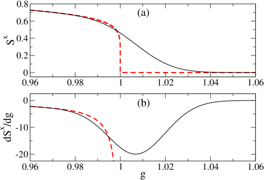
Figure 1: Longitudinal magnetization and its derivative. In both panels results for inhomogeneous (homogeneous) systems are denoted by the black solid (red dashed) line. The homogeneous results, $S^{x}_{H}$ and $dS^{x}_{H}/dg$, are given by (14) and (15), respectively. The inhomogeneous field is given by (16) with $\lambda_{Q}=5000$.

IV Longitudinal magnetization

Longitudinal magnetization and its derivative are plotted in Fig. 1. It is clear from this plot that magnetization $S^{x}$, unlike its homogeneous counterpart $S^{x}_{H}$, is featureless around the critical point. It smoothly decreases reaching zero far away from the critical point on the paramagnetic side of the phase diagram (Fig. 1a). The most efficient way to estimate the position of the critical point from such data is to compute the derivative of $S^{x}$, which exhibits the minimum near the critical point in the paramagnetic phase (Fig. 1b). It is therefore quite interesting to find out how accurately one may extrapolate the position of the critical point from such data.

Since the singularity of $dS_{H}^{x}/dg$ is algebraic (15), we use scaling ansatz (7) to study the extremum of $dS^{x}/dg$. It then immediately follows that this extremum should be located at $g_{x}^{*}$ such that

$$|g_{x}^{*}-g_{c}|\sim\hat{g}\sim\lambda_{Q}^{-1/(1+\nu)}.\\$$ (18)

Moreover, we also expect from (7) that

$$\frac{dS^{x}}{dg}(g_{x}^{*})\sim{\hat{x}}^{\gamma/\nu}\sim\lambda_{Q}^{\gamma/(1+\nu)}.$$ (19)

These scaling predictions will be verified below. Before moving on, however, we would like to note that the scaling relation (19) involves the exponent $\gamma=7/8$, which is defined only on the ferromagnetic side of the transition (15). Therefore, it should not be taken for granted that the scaling of $dS^{x}/dg$ at the minimum, which is located in the paramagnetic phase, is given by relation (19).

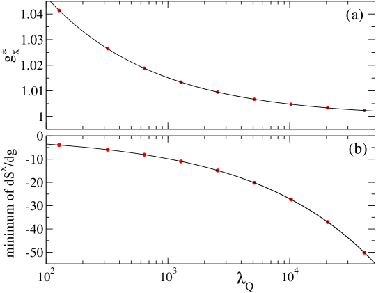
Figure 2: Scaling properties of the minimum of $dS^{x}/dg$. Panel (a): position $g^{*}_{x}$ of the minimum. Red dots provide numerical data. The black line is the non-linear fit yielding $g^{*}_{x}=0.99985(3)+0.440(2)\lambda_{Q}^{-0.487(1)}$. Panel (b): minimum of $dS^{x}/dg$. Red dots provide numerical data, while the black line is the non-linear fit: minimum of $dS^{x}/dg=0.095(3)-0.4845(4)\lambda_{Q}^{0.43705(7)}$. The fitted coefficients and their standard errors, both here and in other plots in this work, come from NonlinearModelFit function from Mat . We report everywhere in this paper one standard error in the brackets next to the fitted coefficients.

The scaling of $g^{*}_{x}$ is presented in Fig. 2a. We fit there $g^{*}_{x}$ with

$$a+b\lambda_{Q}^{c}.$$ (20)

The parameter $a$ extrapolates the position of the critical point to the infinite $\lambda_{Q}$ limit, where the system becomes effectively homogeneous ($c<0$). We obtain $a\approx 0.99985$, which proves that susceptibility $dS^{x}/dg$ in the spatially inhomogeneous system can be efficiently used for finding the critical point.

The parameter $c$, according to (18), should be compared to $-1/(1+\nu)=-1/2$. The fitted exponent $c\approx-0.487$ is in a good agreement with the spatial KZ scaling arguments employed in ansatz (7). Its actual value depends on the range of $\lambda_{Q}$’s used for the fit. We used $\lambda_{Q}\in(10^{2},5\cdot 10^{5})$ to obtain such a value. Increase of the lowest $\lambda_{Q}$’s used for the fit, brings the exponent $c$ closer to the expected value of $-1/2$. This is in agreement with the expectation that KZ scaling predictions work best in the limit of $\lambda_{Q}\to\infty$. The same happens in time quenches, where the KZ predictions best fit the non-equilibrium data in the limit of $\tau_{Q}\to\infty$ as long as finite-size effects are negligible, which happens for Jac (a)

$$N\gg\hat{\xi}.$$ (21)

Note the similarity between the conditions for irrelevance of finite-size effects in spatial (17) and time (21) quenches.

The scaling of the value of $dS^{x}/dg$ at the minimum is illustrated in Fig. 2b. Fit (20) to the numerical data provides the exponent $c\approx 0.43705$, which is in excellent agreement with the expected $\gamma/(1+\nu)=7/16=0.4375$ from (19). This happens despite the above-mentioned problems with assigning the value to the exponent $\gamma$ on the paramagnetic side of the transition.

Looking at these results, we see an immediate analogy to the ones that are obtained in homogeneous but finite-size systems Car (a, b). In such systems susceptibilities also exhibit an extremum near the critical point. Such an extremum moves towards the critical point when the system size increases. The extrapolation of its position to the thermodynamic limit provides the critical point. The algebraic in the system size scaling of its distance and value encodes the critical exponents $\nu$ and $\gamma$, respectively.

V Transverse magnetization

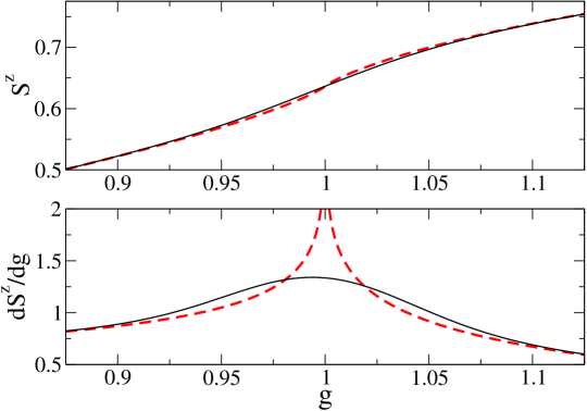
Figure 3: Transverse magnetization and its derivative. In both panels results for inhomogeneous (homogeneous) systems are denoted by the solid black (dashed red) line. The homogeneous results $S^{z}_{H}$ and $dS_{H}^{z}/dg$ are given by (12) and (34), respectively. The inhomogeneous results come from numerics done for $\lambda_{Q}=320$.

Transverse magnetization $S^{z}$ and its derivative $dS^{z}/dg$ are plotted in Fig. 3. It is interesting to note that even in the thermodynamically-large homogeneous system $S^{z}_{H}$, unlike $S^{x}_{H}$, does not reveal where the critical point is until we compute its derivative. The derivative of transverse magnetization is quite different from the derivative of longitudinal magnetization in both homogeneous and spatially driven systems. Instead of a minimum on the paramagnetic side of the transition, there is a maximum of $dS^{z}/dg$ in the ferromagnetic phase. $dS^{z}_{H}/dg$ is non-zero on both sides of the critical point unlike $dS^{x}_{H}/dg$. Most importantly, however, $dS^{z}_{H}/dg$ is logarithmically rather than algebraically divergent at the critical point.

Therefore, we need to replace ansatz (7) to properly take care of the logarithmic singularity (13) at the critical point of the homogeneous system. To derive the appropriate ansatz, we adopt to our observable the RG approach developed in Tur (a). We start by noting that relation (2) implies that under the change of the length scale by a factor $b$, $g$ is mapped to $g^{\prime}$ in a homogeneous system such that Car (b)

$$g^{\prime}-g_{c}=(g-g_{c})b^{1/\nu}.$$ (22)

Thus, if $O_{H}(g-g_{c})$ is given by (13), then the scale transformation leads to

$$O_{H}(g^{\prime}-g_{c})=O_{H}(g-g_{c})-\frac{\ln b}{\pi\nu}.$$ (23)

The scale transformation in the inhomogeneous system results in

$$x^{\prime}-x_{c}=(x-x_{c})b^{-1},\ \ \lambda_{Q}^{\prime}=\lambda_{Q}b^{-(1+\nu)/\nu},$$

where the first relation is obvious, while the second one is discussed in Tur (a). Next, we assume that the transformation law (23) applies also to observable $O$ in an inhomogeneous system sufficiently close to the critical point. This allows us to write

$$O(x-x_{c},\lambda_{Q})=O\!\left((x-x_{c})b^{-1},\lambda_{Q}b^{-(1+\nu)/\nu}\right)+\frac{\ln{b}}{\pi\nu}.$$ (24)

One way to find the scaling solution of that equation is to notice that its left-hand-side is independent of $b$ and so its derivative with respect to $b$ is zero. This allows us to write the differential equation for $O$

$$A\frac{\partial O(A,B)}{\partial A}+\frac{\nu+1}{\nu}B\frac{\partial O(A,B)}{\partial B}=\frac{1}{\pi\nu}.$$

Its regular at $x=x_{c}$ solution reads

$$O(A,B)=f\!\left(AB^{-\nu/(1+\nu)}\right)+\frac{\ln B}{\pi(1+\nu)},$$ (25)

where $f$ is an analytic function at the critical point because we do not anticipate criticality-induced singularities in an inhomogeneous system. Alternatively, one may explore the independence of the left-hand-side of (24) on the scale factor $b$ by putting $b\sim\lambda_{Q}^{\nu/(1+\nu)}$ into the RHS of that equation. This leads to the same solution as (25). As this is a quicker approach, we will follow it in the subsequent calculations.

In the end, we set $\nu=1$, $O=dS^{z}/dg$, and use (3) and (4) to arrive at

$$\frac{dS^{z}}{dg}=f\!\left(\frac{g-g_{c}}{\hat{g}}\right)+\frac{\ln\lambda_{Q}}{2\pi}.$$ (26)

Such an ansatz is quite different from the one provided in (7) and we test it below. Our findings are illustrated in Figs. 4 and 5.

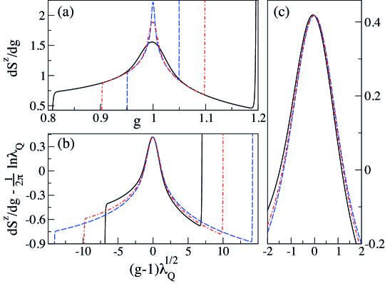
Figure 4: Test of ansatz (26). Panel (a): $dS^{z}/dg$ before rescaling for $\lambda_{Q}$ equal to $1280$ (solid black), $10240$ (dashed-dotted red), and $81910$ (dashed blue). Panel (b): the rescaled version of the panel (a). Panel (c): the same as in the panel (b) but focused around the maximum. The sharp increase of curves in panels (a) and (b) is caused by open boundary conditions, which are imposed at $g$ equal to $1\pm 0.2$ ($\lambda_{Q}=1280$), $1\pm 0.1$ ($\lambda_{Q}=10240$), and $1\pm 0.05$ ($\lambda_{Q}=81910$).

To start discussion of ansatz (26), we note that it contains the KZ-related physics in two places. First, the argument of the scaling function $f$ depends in the expected way on the KZ driving-induced field-scale $\hat{g}\sim 1/\sqrt{\lambda_{Q}}$. Second, the logarithmic in $\lambda_{Q}$ shift on the RHS of (26) can be also linked to the KZ theory. To explain it, we invoke the adiabatic-impulse approximation frequently employed in the context of the KZ theory of non-equilibrium time quenches. This rather crude approximation assumes that in the crossover region between the two adiabatic regimes the state of the system is frozen, i.e., it does not change in the vicinity of the critical point. Adopting such an approximation to the spatial quench, we would assume that in the crossover region, where the local homogeneous approximation breaks down, we have

$$\frac{dS^{z}}{dg}[g(x)]\approx\frac{dS^{z}_{H}}{dg}(g_{c}\pm\hat{g})\approx\text{const}+\frac{\ln\lambda_{Q}}{2\pi}\ \ \ \text{for}\ \ \ |x-x_{c}|\lesssim\hat{x}$$ (27)

after using (13). While such a rough approximation says nothing about the location of the maximum of $dS^{z}/dg$, it properly predicts the scaling of $dS^{z}/dg$ at the maximum. This is seen by comparing (27) to fit (29), which we will discuss below. The adiabatic-impulse predictions always have to be taken with a grain of salt Fra , which does not change the fact that they often times provide a very reasonable lowest-order non-trivial approximation (see e.g. BDP (c); BDp ).

Next, we proceed by subtracting $\ln\lambda_{Q}/2\pi$ from $dS^{z}/dg$ followed by shifting and rescaling of the magnetic field

$$g\mapsto(g-1)\sqrt{\lambda_{Q}}.$$ (28)

We expect that after these transformations, data for different $\lambda_{Q}$’s should collapse on a single curve, whose shape is given by the scaling function $f$. Fig. 4, however, shows that the overlap of the curves is not perfect, despite the fact that fairly high $\lambda_{Q}$’s are considered.

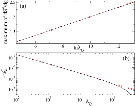
Figure 5: Scaling properties of the maximum of $dS^{z}/dg$. Panel (a): Red dots provide numerical data, while the black line is the linear fit: maximum of $dS^{z}/dg=0.425(1)+0.1584(1)\ln\lambda_{Q}$. Panel (b): the position $g^{*}_{z}$ of the maximum. Red dots provide numerical data, while the black line comes from the non-linear fit $g^{*}_{z}=1.00001(3)-0.951(6)\lambda_{Q}^{-0.873(1)}$.

To look more quantitatively at ansatz (26), we study $dS^{z}/dg$ at the maximum. Ansatz (26) predicts that we should be expecting to find

$$\text{const}+\frac{\ln\lambda_{Q}}{2\pi}.$$

In agreement with this prediction, we observe that the maximum of $dS^{z}/dg$ can be very well fitted with

$$A+B\ln\lambda_{Q},$$ (29)

where $A\approx 0.425$ and $B\approx 0.1584$ (Fig. 5a). Quite interestingly, the value of $B$ very well matches the expected $1/2\pi\approx 0.159$.

Turning now our attention to the position $g^{*}_{z}$ of the maximum of $dS^{z}/dg$, we fit it with (20) getting $a\approx 1.00001$, $b\approx-0.951$, and $c\approx-0.873$ (Fig. 5b). Similarly as in Sec. IV, we obtain an excellent extrapolation of the position of the critical point through the $a$ parameter. The value of the exponent $c$, however, is surprising. Indeed, our expectation based on ansatz (26) was that we would get $-1/(1+\nu)=-1/2$ instead. It should be also noticed that the curve fitted in Fig. 5b does not match numerics for large enough $\lambda_{Q}$, which casts doubt on the power-law scaling of $1-g^{*}_{z}$ with $\lambda_{Q}$.

To resolve these issues, we propose to modify the renormalization procedure taking full advantage of the knowledge of the exact expression for the derivative of magnetization in the homogeneous system. To proceed, we write

$$\frac{dS^{z}_{H}}{dg}=\left.\frac{dS^{z}_{H}}{dg}\right|_{\text{reg}}-\frac{\chi_{H}(g)}{\pi}\ln|g-1|,$$ (30)

where the first (second) term on the RHS is regular (singular) at $g=1$. We mean by regularity that the function itself and all its derivatives are finite. The $\chi_{H}(g)$ function is also regular at $g=1$, so that singularity of $dS^{z}_{H}/dg$ comes solely from the logarithm. $\chi_{H}(g)$ and $\left.dS^{z}_{H}/dg\right|_{\text{reg}}$ are given by (35) and (36), respectively.

Next, we define the observable $O$ in the inhomogeneous system as

$$O=\!\left(\frac{dS^{z}}{dg}-\left.\frac{dS^{z}_{H}}{dg}\right|_{\text{reg}}\right)/\chi_{H}(g).$$

Its homogeneous system analogue $O_{H}$ is obtained by replacing $dS^{z}/dg$ by $dS^{z}_{H}/dg$. It is then immediately seen that $O_{H}$ transforms under the change of scale (22) in the same way as (23). Therefore, we again assume that $O$ transforms in the same way as $O_{H}$ at least near the spatial critical point. Repeating the above-performed steps, we arrive at the new scaling ansatz for $dS^{z}/dg$, which we write in the following way

$$f\!\left(\frac{g-g_{c}}{\hat{g}}\right)=\!\left(\frac{dS^{z}(g)}{dg}-\left.\frac{dS^{z}_{H}(g)}{dg}\right|_{\text{reg}}\right)/\chi_{H}(g)-\frac{\ln\lambda_{Q}}{2\pi}.$$ (31)

This ansatz reproduces ansatz (26) when $\left.dS^{z}_{H}/dg\right|_{\text{reg}}$ and $\chi_{H}$ are evaluated at $g=1$ because $\chi_{H}(1)=1$ and $\left.dS^{z}_{H}/dg\right|_{\text{reg}}$ at $g=1$ can be absorbed into the scaling function $f$. This follows from the fact that in the derivation of ansatz (26), we have assumed that $O_{H}$ is given by (13). Such an approximation is valid only extremely close to the critical point. We overcome this limitation in the derivation of the ansatz (31) using the exact solution for a homogeneous system.

If we now plot the RHS of (31) for different $\lambda_{Q}$’s and rescale the horizontal axis according to (28), we find a wonderful collapse of different curves (Fig. 6). Its most remarkable feature is that it happens not only close to the critical point, but also far away from it. Comparing Figs. 4 and 6, we immediately see that ansatz (31) is significantly better than ansatz (26).

Next, we note that ansatz (31) reproduces exactly the homogeneous result (30) when

$$f(x)=-\frac{\ln|x|}{\pi}.$$ (32)

Therefore, we expect that far away from the critical point, where the local homogeneous approximation is supposed to work, the scaling function from (31) is accurately given by (32). Far away, in the light of the KZ theory, means that $|g-1|/\hat{g}\sim|g-1|\sqrt{\lambda_{Q}}\gg 1$. This is confirmed in Fig. 6a.

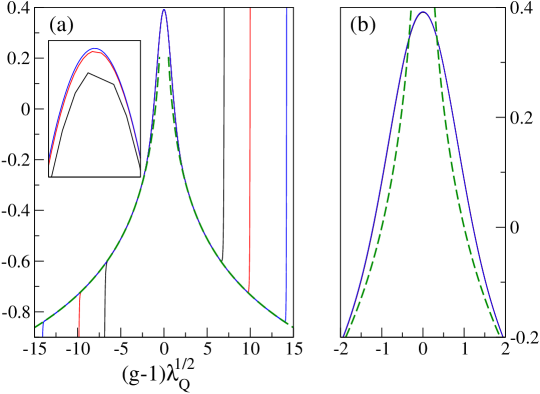
Figure 6: Test of ansatz (31). Panel (a): solid lines depict RHS of (31) for different $\lambda_{Q}$’s. The inset enlarges the extremum. The range of its horizontal and vertical axes is [-0.1,0.1] and [0.387,0.3924], respectively. Panel (b): the same as in the panel (a) but focused around the maximum. The green dashed line in both panels is given by (32). Results for $\lambda_{Q}$ equal to $1280$, $10240$, and $81910$ are depicted with black, red, and blue curves, respectively. The curves overlap so well, that they are practically indistinguishable in the central parts of both panels. The data for $dS^{z}/dg$, used to prepare this plot, is the same as in Fig. 4a.

Finally, we discuss what ansatz (31) predicts for the scaling of the position of the maximum of $dS^{z}/dg$ with $\lambda_{Q}$. To proceed, we parametrize the scaling function around the maximum as

$$f(x)=ax^{2}+bx+c,$$

where $a$, $b$, and $c$ are some constants, and substitute the expressions for $\chi_{H}$ (35) and $\left.dS_{H}^{z}/dg\right|_{\text{reg}}$ (36) into (31) to obtain $dS^{z}/dg$ out of this equation. Next, we compute from such an expression $d^{2}S^{z}/dg^{2}$, expand it in a Taylor series around $g=1$ up to the linear in $g-1$ terms, and equal the resulting expression to zero. This gives us the expression for the position $g^{**}_{z}$ of the extremum of $dS^{z}/dg$. The subsequent discussion can be conveniently done by focusing on the distance $z^{**}$ of the maximum from the critical point expressed in lattice spacing units:

$$z^{**}=(1-g_{z}^{**})\lambda_{Q}.$$

We get

$$z^{**}=\frac{4(4b\pi\sqrt{\lambda_{Q}}-3\ln\lambda_{Q}-6c\pi-6\ln 8+14)}{32a\pi-\frac{48b\pi}{\sqrt{\lambda_{Q}}}+33\frac{\ln\lambda_{Q}}{\lambda_{Q}}+\frac{66c\pi+66\ln 8-154}{\lambda_{Q}}}.$$ (33)

The large $\lambda_{Q}$ scaling of (33) is $b\sqrt{\lambda_{Q}}/2a$, which is in disagreement with numerical simulations, where $z^{*}=(1-g^{*}_{z})\lambda_{Q}$ grows approximately linearly in $\ln\lambda_{Q}$ (Fig. 7). Two remarks are in order now.

First, the logarithmic growth of $z^{*}$ comes as a surprise if we look at this result from the perspective of the KZ theory. The natural expectation would be that $z^{*}\sim\hat{g}\lambda_{Q}\sim\sqrt{\lambda_{Q}}$. It does not, however, imply that the KZ scalings are absent in ansatz (31). As we have explained above, they are present in the argument of the scaling function $f$ and the term $\sim\ln\lambda_{Q}$ on the RHS of (31). In fact, given an excellent overlap of curves in Fig. 6, the KZ scalings are visible not only close to the critical point, but everywhere in the system as long as we stay away from the points where the boundary conditions are imposed.

Second, the logarithmic scaling of $z^{**}$ is obtained from (33) when $b=0$. Therefore, we set $b=0$ and get $a$ and $c$ coefficients from the fit to the data rescaled in the same way as in Fig. 6. The fits done for $\lambda_{Q}\in(5\cdot 10^{3},4\cdot 10^{5})$ around the maximum yield $a=-0.443(3)$ and $c=0.392(1)$. $z^{**}$ for these parameters is plotted in Fig. 7. We see from this figure that $z^{*}$ and $z^{**}$ exhibit the same logarithmic growth with $\lambda_{Q}$. They are, however, systematically shifted by about $0.16$ in lattice units (inset of Fig. 7). We do not see an explanation for this curious shift of about $1/2\pi$; we have extensively checked our numerical and analytical computations to make sure that they are technically correct.

It should be stressed that data for $z^{**}$ comes from the RG calculation that is certainly not expected to give definite predictions with accuracy smaller than the distance between the lattice sites. Indeed, the RG theory captures universal long-wavelength behavior of the system rather than the short-wavelength non-universal one. In fact, it is in our opinion very interesting that the discrepancy between the RG result and the exact numerical one is so tiny.

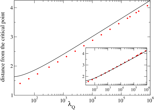
Figure 7: Distance of the maximum of $dS^{z}/dg$ from the critical point in the lattice spacing units. The red dots show numerics, i.e., $z^{*}=(1-g^{*}_{z})\lambda_{Q}$. The black solid line shows $z^{**}$ for $a=-0.443$, $b=0$, $c=0.392$; see (33). The inset shows the same as the main plot, but after shifting data for $z^{*}$ by $0.16$.

VI Summary

We have comprehensively studied derivatives of longitudinal and transverse magnetizations in the inhomogeneous Ising model. We have shown that both these quantities exhibit an extremum that can be efficiently used for finding the position of the critical point of the homogeneous Ising chain.

Properties of the extremum of the derivative of longitudinal magnetization are captured by power law scalings with the gradient of the external field. These scaling relations encode universal critical exponents. As a result, the correlation length and longitudinal magnetization critical exponents, characterizing some singularities of the homogeneous Ising chain, can be obtained from the studies of such an extremum in the inhomogeneous system.

The scaling properties of the extremum of the derivative of transverse magnetization in the inhomogeneous system are rather complicated. Their proper description have required detailed knowledge of the exact solution in the homogeneous chain. The key difference between derivatives of longitudinal and transverse magnetizations is that in the homogeneous system the former exhibits a power law singularity while the latter has a logarithmic singularity. It is a bit surprising that this makes such a difference in the theoretical description of these derivatives in the inhomogeneous system.

Besides exact diagonalization and renormalization group theory, one may apply the Kibble-Zurek approach to the inhomogeneous Ising chain. Predictions of this intuitive approach are easily seen in the derivative of longitudinal magnetization. Some of them are also present in the derivative of transverse magnetization, but there is no straightforward way of extracting them.

We believe that it would be interesting to extend these studies to other systems to gain better understanding of quantum phase transitions in inhomogeneous fields. Such studies should be useful in the context of cold atom and ion experiments, where inhomogeneities of external fields are ubiquitous and strongly-correlated models describing these systems are typically not exactly solvable Lew ; Blo . To experimentally study the critical points and exponents in these systems, one may try to minimize inhomogeneities disturbing their quantum phase transitions. This, however, may not always be feasible (e.g. the external trapping potential acting on cold atoms and ions is present in nearly all current experiments). The other option is to control inhomogeneous fields and study susceptibilities along the lines suggested in this work.

Appendix A Transverse magnetization in homogeneous Ising chain

It is convenient to introduce the following notation

$$G=\frac{2\sqrt{g}}{1+g},\ \ \tilde{G}=\sqrt{1-G^{2}}=\frac{|1-g|}{1+g},\ \ 0\leq G,\tilde{G}\leq 1.$$

The ground-state energy per lattice site in the thermodynamically-large homogeneous system is Lie

$${\cal E}_{H}=-\frac{1}{\pi}\int_{0}^{\pi}dk\sqrt{1+g^{2}-2g\cos(k)}=-\frac{2}{\pi}(1+g)E(G),$$

where

$$E(x)=\int_{0}^{\pi/2}dk\sqrt{1-x^{2}\sin^{2}(k)}$$

is the complete elliptic integral of the second kind Old . Transverse magnetization is then given through the Feynman-Hellmann theorem, $S^{z}_{H}=-d{\cal E}_{H}/dg$, which leads to (12).

The derivative of transverse magnetization then reads

$$\frac{dS_{H}^{z}}{dg}=-\frac{d^{2}{\cal E}_{H}}{dg^{2}}=\frac{(1+g^{2})K(G)-(1+g)^{2}E(G)}{g^{2}(1+g)\pi},$$ (34)

where

$$K(x)=\int_{0}^{\pi/2}\frac{dk}{\sqrt{1-x^{2}\sin^{2}(k)}}$$

is the complete elliptic integral of the first kind Old .

Next, we need to factor out singular and regular at $g=1$ parts of elliptic integrals from (34). Using identities from Sec. 61:6 of Old , we get

$$\left.K(G)\right.=\left.K(G)\right|_{\text{sing}}+\left.K(G)\right|_{\text{reg}},$$

$$\left.K(G)\right|_{\text{sing}}=-\frac{2}{\pi}K(\tilde{G})\ln|1-g|,\ \ \left.K(G)\right|_{\text{reg}}=\frac{2}{\pi}K(\tilde{G})\ln[4(1+g)]+2\sum_{j=1}^{\infty}\!\left[\frac{(2j-1)!!}{(2j)!!}\tilde{G}^{j}\right]^{2}\sum_{n=1}^{2j}\frac{(-1)^{n}}{n},$$

$$\left.E(G)\right.=\left.E(G)\right|_{\text{sing}}+\left.E(G)\right|_{\text{reg}},$$

$$\left.E(G)\right|_{\text{sing}}=\frac{2}{\pi}\!\left[E(\tilde{G})-K(\tilde{G})\right]\ln|1-g|,$$

$$\left.E(G)\right|_{\text{reg}}=1+\frac{2}{\pi}\!\left[K(\tilde{G})-E(\tilde{G})\right]\ln[4(1+g)]+2\sum_{j=1}^{\infty}\frac{(2j-1)!!(2j-3)!!}{(2j)!!(2j-2)!!}\tilde{G}^{2j}\!\left[\frac{1}{4j-8j^{2}}+\sum_{n=1}^{2j-2}\frac{(-1)^{n}}{n}\right].$$

Note that $K(\tilde{G})$ and $E(\tilde{G})$ are regular at $g=1$ Old . These equations allow us to split $dS^{z}_{H}/dg$ into singular

$$\left.\frac{dS_{H}^{z}}{dg}\right|_{\text{sing}}=-\frac{\chi_{H}(g)}{\pi}\ln|1-g|,$$ (35)

$$\left.\chi_{H}(g)\right.=\frac{2}{g^{2}(1+g)\pi}\!\left[(1+g)^{2}E(\tilde{G})-2gK(\tilde{G})\right]=1+O(g-1),$$

and regular parts

$$\left.\frac{dS_{H}^{z}}{dg}\right|_{\text{reg}}=\frac{dS^{z}_{H}}{dg}-\left.\frac{dS^{z}_{H}}{dg}\right|_{\text{sing}}.$$ (36)

The regular part is most conveniently obtained by replacing $K(G)$ and $E(G)$ in (34) by $\left.K(G)\right|_{\text{reg}}$ and $\left.E(G)\right|_{\text{reg}}$, respectively.

References

- (1) T. W. B. Kibble, J. Phys. A 9, 1387 (1976); Phys. Rep. 67,183 (1980).
- (2) W. H. Zurek, Nature (London) 317, 505 (1985); W.H. Zurek, Phys. Rep. 276, 177 (1996).
- (3) T. W. B. Kibble, Phys. Today 60, 47 (2007); A. del Campo, T. W. B. Kibble, and W. H. Zurek, J. Phys.: Condens. Matter 25, 404210 (2013); A. del Campo and W. H. Zurek, Int. J. Mod. Phys. A 29, 1430018 (2014).
- BDP (a) B. Damski, Phys. Rev. Lett. 95, 035701 (2005).
- Dor (a) W. H. Zurek, U. Dorner, and P. Zoller, Phys. Rev. Lett. 95, 105701 (2005).
- Jac (a) J. Dziarmaga, Phys. Rev. Lett. 95, 245701 (2005).
- Pol (a) A. Polkovnikov, Phys. Rev. B 72, 161201(R) (2005).
- Jac (b) J. Dziarmaga, Adv. Phys. 59, 1063 (2010).
- Pol (b) A. Polkovnikov, K. Sengupta, A. Silva, and M. Vengalattore, Rev. Mod. Phys. 83, 863 (2011).
- (10) A. Dutta, G. Aeppli, B. K. Chakrabarti, U. Divakaran, T. F. Rosenbaum, and D. Sen, Quantum Phase Transitions in Transverse Field Spin Models: From Statistical Physics to Quantum Information (Cambridge University Press, 2015); arXiv:1012.0653.
- Tur (a) T. Platini, D. Karevski, and L. Turban, J. Phys. A: Math. Theor. 40, 1467 (2007).
- Dor (b) W. H. Zurek and U. Dorner, Phil. Trans. R. Soc. A366, 2953 (2008).
- Tur (b) M. Collura, D. Karevski, and L. Turban, J. Stat. Mech. (2009) P08007.
- (14) B. Damski and W. H. Zurek, New J. Phys. 11, 063014 (2009).
- (15) M. Campostrini and E. Vicari, Phys. Rev. A 81, 023606 (2010).
- (16) S. Suzuki and A. Dutta, Phys. Rev. B 92, 064419 (2015).
- Jac (c) J. Dziarmaga and M. M. Rams, New J. Phys. 12 055007 (2010); New J. Phys. 12, 103002 (2010).
- (18) M. Collura and D. Karevski, Phys. Rev. Lett. 104, 200601 (2010); Phys. Rev. A 83, 023603 (2011).
- (19) M. M. Rams, M. Mohseni, and A. del Campo, New J. Phys. 18, 123034 (2016).
- (20) M. Lewenstein, A. Sanpera, and V. Ahufinger, Ultracold Atoms in Optical Lattices: Simulating Quantum Many-Body Systems (Oxford University Press, Oxford, UK, 2012).
- (21) I. Bloch, J. Dalibard, and W. Zwerger, Rev. Mod. Phys. 80, 885 (2008).
- Car (a) J. L. Cardy, ed., Finite-Size Scaling (North-Holland, Amsterdam, 1988).
- (23) M. Kolodrubetz, B. K. Clark, and D. A. Huse, Phys. Rev. Lett. 109, 015701 (2012).
- (24) A. Chandran, A. Erez, S. S. Gubser, and S. L. Sondhi, Phys. Rev. B 86, 064304 (2012).
- (25) A. Francuz, J. Dziarmaga, B. Gardas, and W. H. Zurek, Phys. Rev. B 93, 075134 (2016).
- BDP (b) B. Damski and W. H. Zurek, Phys. Rev. Lett. 104, 160404 (2010).
- (27) E. Lieb, T. Schultz, and D. Mattis, Ann. Phys. (N.Y.) 16, 407 (1961).
- (28) P. Pfeuty, Ann. Phys. 57, 79 (1970).
- (29) E. Barouch and B. M. McCoy, Phys. Rev. A 3, 786 (1971).
- (30) A. P. Young, Phys. Rev. B 56, 11691 (1997).
- (31) G. F. Giuliani and G. Vignale, Quantum Theory of the Electron Liquid (Cambridge University Press, 2005).
- (32) Wolfram Research, Inc., Mathematica, Version 11.0, Champaign, IL (2016).
- Car (b) J. Cardy, Scaling and Renormalization in Statistical Physics (Cambridge University Press, Cambridge, 2002).
- BDP (c) B. Damski and W. H. Zurek, Phys. Rev. A 73, 063405 (2006).
- (35) B. Damski, Fidelity approach to quantum phase transitions in quantum Ising model, in Quantum Criticality in Con- densed Matter: Phenomena, Materials and Ideas in Theory and Experiment, edited by J. Jedrzejewski (World Scientific, Singapore, 2015), pp. 159–182; arXiv:1509.03051.
- (36) K. Oldham, J. Myland, and J. Spanier, An Atlas of Functions, 2nd ed. (Springer, 2009).