Single spin detection with an ensemble of probe spins

Abstract

Single spin detection is a key objective in the field of metrology. There have been many experimental and theoretical investigations for the spin detection based on the use of probe spins. A probe spin shows the precession due to dipole-dipole interaction from a target spin, and measurement results of the probe spin allow us to estimate the state of the target spin. Here, we investigate performance of single-spin detection when using an ensemble of probe spins. Even though the ensemble of probe spins inevitably induces projection noise that could hinder the signal from the target spin, optimization of the configuration of the spin ensemble improves the sensitivity such that enhancement of the signal can be much larger than the projection noise. The probe-spin ensemble is especially useful at a large distance from the target spin , where it is difficult for a single spin to read out the target spin within a reasonable repetition time. Our results pave the way for a new strategy to realize efficient single-spin detections.

An important objective in quantum metrology is to realize the efficient detection of a single spin. This technique has numerous potential applications because we can in principle extract useful information about materials by imaging nuclear magnetism on the nanometer scale. However, such single-spin detection requires both sensitivity and spatial resolution. There have been several experimental and theoretical studies to improve both the sensitivity and spatial resolution of magnetic-field sensors such as SQUID, a superconducting flux qubit, Hall sensors, and force sensors Ramsden (2006); Vasyukov et al. (2013); Bal et al. (2012); Toida et al. (2016); Bienfait et al. (2016). Even though there are some experimental demonstrations of single-spin detection Rugar et al. (2004), single-spin detection is not yet a mature technology . This is a particularly true because many repetitions of the measurements are necessary to increase the signal -to -noise ratio for the spin detection and much more efficient schemes are required to realize rapid spin detection.

The use of a probe spin is one attractive approach for the single-spin detection Degen (2008); Maze et al. (2008); Taylor et al. (2008); Balasubramanian et al. (2008); Schaffry et al. (2011); Müller et al. (2014); Staudacher et al. (2013); Mamin et al. (2013); Ohashi et al. (2013); Rugar et al. (2015). The probe spin can be coupled with the target spin via dipole-dipole interaction, and the probe spin experiences a precession due to the magnetic field induced by the target spin. From an optical or electrical readout of the state of the probe spin , we can estimate the magnitude of the magnetic field applied to the probe spin, which provides us with information on the target spin.

Conversely, there have been several theoretical and experimental studies of ensembles of spins for use as sensitive magnetic-field sensors Vengalattore et al. (2007); Kominis et al. (2003); Acosta et al. (2009); Maertz et al. (2010); Le Sage et al. (2013); Wolf et al. (2015). If we use an ensemble of spins to measure the applied magnetic fields, we can enhance the signal from the target magnetic field. This has a clear advantage over a single- spin field sensor if we aim to detect global magnetic fields. However, an ensemble of spins has projection noise resulting from the intrinsic properties of quantum mechanics where the readout of the quantum states becomes a stochastic process. This problem could be significant if we aim to use the probe-spin ensemble to detect a single target spin. The dipole-dipole interaction between spins has the form $H_{\rm{dd}}\propto 1/r^{3}$ where $r$ denotes the distance between the spins ; therefore, the interaction becomes significantly weaker as we increase the distance from the target spin. This means that, if we use an ensemble of probe spins to detect the target spin, probe spins far from the target spins could induce projection noise without contributing to the enhancement of the signal. Therefore, a careful assessment is required to determine the conditions when a probe-spin ensemble shows better performance than a single probe spin.

In this paper, we investigate performance of the single-spin detection with a probe-spin ensemble. Interestingly, we found that, by choosing a suitable distribution of probe spins, the use of a probe-spin ensemble is much more efficient than that of a single probe spin. As a concrete example, we consider nitrogen vacancy centers. By performing numerical simulations with realistic parameters, we found that the sensitivity of the probe-spin ensemble becomes more than 10 times better than that of the single probe spin.

The remainder of this paper is organized as follows. In Sec. II we review magnetic-field sensing with the standard echo technique. In Sec. III we investigate the performance of single-spin detection using a probe spin. In Sec. IV we introduce a spin detection scheme using an ensemble of probe spins. Finally, in Sec. V, we offer our conclusions.

I Sensing global magnetic fields with a probe spin

Let us review sensing global magnetic fields with a single probe spin using the standard echo measurement. The Hamiltonian is described as

$$H = \frac{\omega-\omega^{\prime}}{2}\hat{\sigma}_{z}+\lambda\hat{\sigma}_{x}\cos(\omega^{\prime}t+\phi)$$

where $\omega=g\mu_{b}B_{\rm{ex}}+g\mu_{b}B(t)$ denotes the resonant frequency of the probe spin, $g$ denotes a g factor, $\mu_{b}$ denotes a Bohr magneton, $B_{\rm{ex}}$ denotes a known external magnetic field, $B(t)$ denotes a target global magnetic field, $\omega^{\prime}=g\mu_{b}B_{\rm{ex}}$ denotes the frequency of the microwave fields, $\lambda$ denotes a Rabi frequency, and $\phi$ denotes the phase of the microwave fields. After applying a rotating wave approximation, we obtain

$$H \simeq \frac{g\mu_{b}B(t)}{2}\hat{\sigma}_{z}+\lambda_{x}\hat{\sigma}_{x}+\lambda_{y}\hat{\sigma}_{y}$$

where $\lambda_{x}$ ($\lambda_{y}$) denotes a Rabi frequency of the microwave along the $x$ ($y$) direction. We turn off the microwave driving ($\lambda_{x}=\lambda_{y}=0$) except when we need to rotate the probe spin. We define $H_{\rm{FID}}=\frac{g\mu_{b}B(t)}{2}\hat{\sigma}_{z}$ for the Hamiltonian without microwave driving. In particular, we consider alternating square fields ( which can be considered to be AC fields Dolde et al. (2011)) described as

$$B(t)=\left\{\begin{array}[]{l}B\ \ (0\leq t<\frac{t_{\rm{I}}}{2})\\ -B(\frac{t_{\rm{I}}}{2}\leq t\leq t_{\rm{I}})\end{array}\right.$$ (5)

where $t_{\rm{I}}$ denotes an interaction between the probe spin and the target magnetic fields. We describe a scheme to estimate the value of $B$ with the probe spin at a given time $T$ ( see Fig. 1).

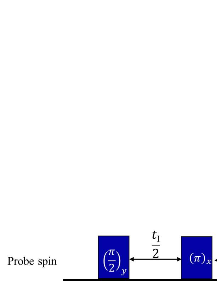
Figure 1: Pulse sequence to detect global AC magnetic fields using the spin echo technique. The $\pi$ pulse in the middle improves the coherence time of the probe spin, because it removes the low frequency noise.

First, we prepare a state of $|\psi_{0}\rangle=|+\rangle=\frac{1}{\sqrt{2}}(|0\rangle+|1\rangle)$ by performing $\frac{\pi}{2}$ pulse along the $y$ direction. Second, we allow this state to evolve with the Hamiltonian $H_{\rm{FID}}$ for time $\frac{t_{\rm{I}}}{2}$. Because the probe spins are affected by dephasing from the environment, the non-diagonal terms of the density matrix decay. Taking this decoherence into consideration, the density matrix after the evolution at time $t$ is given as $\rho(t)=\frac{1}{2}|0\rangle\langle 0|+\frac{1}{2}e^{-ig\mu_{b}Bt-\gamma t}|1\rangle\langle 0|+\frac{1}{2}e^{ig\mu_{b}Bt-\gamma t}|0\rangle\langle 1|+\frac{1}{2}|1\rangle\langle 1|$ where $\gamma$ denotes the dephasing rate. Third, after performing a $\pi$ pulse along the $x$ axis to flip the probe spin at time $t=\frac{t_{\rm{I}}}{2}$, we allow this state to evolve with the Hamiltonian $H_{\rm{FID}}$ for time $\frac{t_{\rm{I}}}{2}$. Note that this $\pi$ pulse at $t=\frac{t_{\rm{I}}}{2}$ suppresses the low-frequency fluctuations of the resonant frequency of the probe spin, which improves the coherence time De Lange et al. (2010). Fourth, we perform a projective measurement on this state about an observable $\hat{\sigma}_{y}$, which can be realized by a $\hat{\sigma}_{z}$ measurement after a $\frac{\pi}{2}$ pulse along the $x$ direction. The expectation value is calculated as $\langle\hat{\sigma}_{y}\rangle=e^{-\gamma t_{\rm{I}}}\sin g\mu_{b}Bt_{\rm{I}}\simeq e^{-\gamma t}g\mu_{b}Bt_{\rm{I}}$ where we use $\omega t_{\rm{I}}\ll 1$. Finally, we repeat the above three steps within a given time $T$. We assume that the necessary time for the single qubit rotation and the measurements is much shorter than the coherence time of the probe spins. In this case, the number of trials in a given time $T$ is approximated as $N\simeq T/t_{\rm{I}}$. We can calculate the uncertainty of the estimation of the magnetic fields as follows :

$$\delta B = \frac{\sqrt{\langle\delta\hat{\sigma}_{y}\delta\hat{\sigma}_{y}\rangle}}{|\frac{d\langle\hat{\sigma}_{y}\rangle}{dB}|}\frac{1}{\sqrt{N}}$$

where $\delta\hat{\sigma}_{y}\equiv\hat{\sigma}_{y}-\langle\hat{\sigma}_{y}\rangle$. If the magnetic fields are small, we can simplify the uncertainty as $\delta B\simeq\frac{1}{e^{-t_{\rm{I}}/T_{2}}g\mu_{b}t_{\rm{I}}}\frac{1}{\sqrt{\frac{T}{t_{\rm{I}}}}}$ where $T_{2}=\frac{1}{\gamma}$ denotes the coherence time. We can minimize this uncertainty by choosing $t=\frac{T_{2}}{2}$, and thus obtain $\delta B_{\rm{min}}\simeq\frac{1}{e^{-\frac{1}{2}}g\mu_{b}}\frac{1}{\sqrt{\frac{T_{2}T}{2}}}$.

II Single-spin detection using a single probe spin.

We now consider detecting a target spin using a single probe spin. When the target spin is located at the origin of the coordinate system, the Hamiltonian between the target spin and the probe spin is described as follows :

$$H = H_{\rm{e}}+H_{\rm{I}}+H_{\rm{t}}$$

$$H_{\rm{e}} = \frac{g_{\rm{e}}\mu_{b}B_{\rm{ex}}}{2}\hat{\sigma}^{(\rm{e})}_{z}+\lambda^{(\rm{e})}\hat{\sigma}^{(\rm{e})}_{x}\cos(\omega^{\prime}t+\phi^{\prime})$$

$$H_{\rm{I}} = G\frac{1}{|\mathbf{r}|^{3}}\Big{(}3\frac{1}{|\mathbf{r}^{2}|}(\mathbf{\sigma^{(e)}}\cdot\mathbf{r})(\mathbf{\sigma^{(t)}}\cdot\mathbf{r})-(\mathbf{\sigma^{(e)}}\cdot\mathbf{\sigma^{(t)}})\Big{)}$$

$$H_{\rm{t}} = \frac{g_{\rm{t}}\mu_{b}B_{\rm{ex}}}{2}\hat{\sigma}^{(\rm{t})}_{z}+\lambda^{(\rm{t})}\hat{\sigma}^{(\rm{t})}_{x}\cos(\omega^{\prime\prime}t+\phi^{\prime\prime})$$

where $B_{\rm{ex}}$ denotes the external magnetic fields, $\lambda^{(\rm{e})}$($\lambda^{(\rm{t})}$) denotes a Rabi frequency for the probe (target) spin, $\omega^{\prime}=g_{\rm{e}}\mu_{b}B_{\rm{ex}}$ ($\omega^{\prime\prime}=g_{\rm{t}}\mu_{b}B_{\rm{ex}}$) denotes the frequency of the microwave fields on the probe (target) spin, $\phi^{\prime}$ ($\phi^{\prime\prime}$) denotes the phase of the microwave fields, and $\mathbf{r}=(x,y,z)$ denotes the position of the probe spin. In addition, we have $\mathbf{\sigma^{(e)}}\cdot\mathbf{r}=x\hat{\sigma}^{(\rm{e})}_{x}+y\hat{\sigma}^{(\rm{e})}_{y}+z\hat{\sigma}^{(\rm{e})}_{z}$ and $\mathbf{\sigma^{(t)}}\cdot\mathbf{r}=x\hat{\sigma}^{(\rm{t})}_{x}+y\hat{\sigma}^{(\rm{t})}_{y}+z\hat{\sigma}^{(\rm{t})}_{z}$. For $g_{\rm{e}}\mu_{b}B_{\rm{ex}}\gg g_{\rm{t}}\mu_{b}B_{\rm{ex}}$, we use a rotating wave approximation, and simplify the Hamiltonian in a rotating frame as

$$H_{\rm{e}} \simeq \lambda_{x}^{(\rm{e})}\hat{\sigma}^{(\rm{e})}_{x}+\lambda^{(\rm{e})}_{y}\hat{\sigma}^{(\rm{e})}_{y}$$

$$H_{\rm{I}} \simeq \frac{G}{(x^{2}+y^{2}+z^{2})^{\frac{3}{2}}}(\frac{3z^{2}}{x^{2}+y^{2}+z^{2}}-1)\hat{\sigma}^{(\rm{e})}_{z}\hat{\sigma}^{(\rm{t})}_{z}$$

$$H_{\rm{t}} \simeq \lambda_{x}^{(\rm{t})}\hat{\sigma}^{(\rm{e})}_{x}+\lambda^{(\rm{t})}_{y}\hat{\sigma}^{(\rm{e})}_{y}$$ (8)

where $\lambda_{x}^{(\rm{e})}$ ($\lambda_{x}^{(\rm{t})}$) denotes a Rabi frequency along the $x$ component on the probe (target) spin and $\lambda_{y}^{(\rm{e})}$ ($\lambda_{y}^{(\rm{t})}$) denotes a Rabi frequency along the $y$ component on the probe (target) spin. We turn off the microwave driving ($\lambda_{x}^{(\rm{e})}=\lambda_{x}^{(\rm{t})}=\lambda_{y}^{(\rm{t})}=\lambda_{y}^{(\rm{t})}=0$) except when we need to rotate the spins. Because the target is the spin $\frac{1}{2}$, the observable $\hat{\sigma}^{(\rm{t})}_{z}$ provides us with $+1$ or $-1$ depending on the target state after the measurement. We can consider an effective Hamiltonian ,

$$H^{(\rm{eff})}_{\rm{I}}\simeq\frac{G}{(x^{2}+y^{2}+z^{2})^{\frac{3}{2}}}(\frac{3z^{2}}{x^{2}+y^{2}+z^{2}}-1)s\hat{\sigma}^{(\rm{e})}_{z}$$ (9)

where $\hat{\sigma}^{(\rm{t})}_{z}$ is replaced by a classical parameter $s$. In this case, the dipole-dipole interaction from the target spin can be treated as the magnetic fields on the probe spin where the effective Zeeman splitting is defined as

$$B^{\rm{(eff)}}=\frac{2G}{g_{\rm{e}}\mu_{b}(x^{2}+y^{2}+z^{2})^{\frac{3}{2}}}(\frac{3z^{2}}{x^{2}+y^{2}+z^{2}}-1)s$$ (10)

Similar to the global magnetic-field sensing described above, we can estimate the parameter $s$ using the standard echo measurement where we flip the target spin in the middle to induce effective AC magnetic fields, as described in Fig. 2. If we have $s\simeq 1$ ($s\simeq-1$) as the estimated value, we can conclude that the state of the target spin is up (down). Similar to the detection of the global magnetic fields, we can calculate the uncertainty of the estimation of $s$ as follows :

$$\delta s^{\rm{(single)}}\simeq\frac{1}{e^{-\frac{t_{\rm{I}}}{T^{(\rm{single})}_{2}}}\frac{2G}{(x^{2}+y^{2}+z^{2})^{\frac{3}{2}}}|\frac{3z^{2}}{x^{2}+y^{2}+z^{2}}-1|t_{\rm{I}}\sqrt{\frac{T}{t_{\rm{I}}}}}$$ (11)

where $T^{(\rm{single})}_{2}$ denotes the coherence time of the single probe spin. We can minimize this uncertainty by choosing $t_{\rm{I}}=\frac{1}{2}T^{(\rm{single})}_{2}$, and obtain

$$\delta s^{(\rm{single})}_{\rm{min}}\simeq\frac{1}{\frac{2e^{-\frac{1}{2}}G}{(x^{2}+y^{2}+z^{2})^{\frac{3}{2}}}|\frac{3z^{2}}{x^{2}+y^{2}+z^{2}}-1|\sqrt{\frac{TT^{\rm{(single)}}_{2}}{2}}}.$$ (12)

Note that we need to decrease this uncertainty to much smaller than $1$ to determine the state of the target spin.

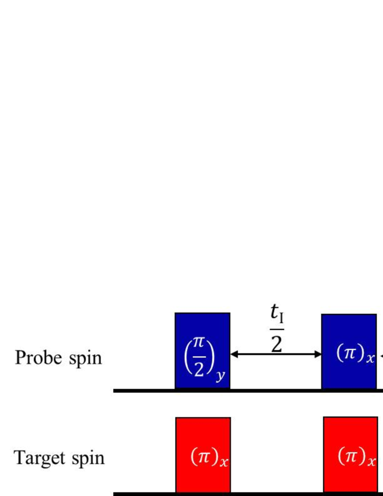
Figure 2: Pulse sequence to detect the state of the target spin with a probe spin. The pulse sequence on the probe spin is the same as that used to detect the AC magnetic fields, as described in Fig. 1. Note that, in order to generate effective AC magnetic fields from the target spin, we perform two $\pi$ pulses on the target spin Mamin et al. (2013).

III Single-spin detection using an ensemble of probe spins

Here,we describe our scheme to detect the target spin with an ensemble of probe spins. In a rotating frame, the effective interaction Hamiltonian between the probe spins and the target spin is given as

$$H^{\rm{(eff)}}_{\rm{I}} \simeq \sum_{j=1}^{L}\frac{g_{\rm{e}}\mu_{b}B_{j}}{2}\hat{\sigma}^{(\rm{e})}_{z,j}$$ (13)

$$B_{j} = 2\frac{G}{g_{\rm{e}}\mu_{b}(x_{j}^{2}+y_{j}^{2}+z_{j}^{2})^{\frac{3}{2}}}(\frac{3z_{j}^{2}}{x_{j}^{2}+y_{j}^{2}+z_{j}^{2}}-1)s$$

where $B_{j}$ denotes the effective magnetic fields on the $j$ th probe spins from the target spin, $\mathbf{r}_{j}=(x_{j},y_{j},z_{j})$ denotes the position of the $j$ th probe spin, $L$ denotes the number of probe spins,and $s$ denotes the state of the target spin. We use the same pulse sequence described in Fig. 2, and assume that we can uniformly implement both the $\frac{\pi}{2}$ pulse and the $\pi$ pulse on the all the probe spins. The uncertainty of the estimation for the probe spin ensemble can be calculated as

$$\delta s^{(\rm{ens})} = \frac{\sqrt{\langle\delta\hat{M}_{y}\delta\hat{M}_{y}\rangle}}{|\frac{d\langle\hat{M}_{y}\rangle}{ds}|}\frac{1}{\sqrt{N}}$$

where $\hat{M}_{y}=\sum_{j=1}^{L}\hat{\sigma}_{y}^{(j)}$. We obtain $\langle\hat{M}_{y}\rangle=\sum_{j=1}^{L}e^{-\frac{t_{\rm{I}}}{T^{\rm{(ens)}}_{2}}}\sin(g_{\rm{e}}\mu_{b}B_{j}t_{\rm{I}})\simeq\sum_{j=1}^{L}e^{-\frac{t_{\rm{I}}}{T^{\rm{(ens)}}_{2}}}g_{\rm{e}}\mu_{b}B_{j}t_{\rm{I}}$ where $T_{2}^{\rm{(ens)}}$ denotes the coherence time of the probe-spin ensemble. Taking a continuous limit, we obtain

$$\langle\hat{M}_{y}\rangle\simeq 2G\rho t_{\rm{I}}e^{-\frac{t_{\rm{I}}}{T^{(\rm{ens})}_{2}}}s\int\int\int dxdydz\frac{(\frac{3z^{2}}{x^{2}+y^{2}+z^{2}}-1)}{(x^{2}+y^{2}+z^{2})^{\frac{3}{2}}}$$

where we perform the integral over the region of the probe-spin ensemble by considering the spin density $\rho$. In addition, we obtain $\langle\delta\hat{M}_{y}\delta\hat{M}_{y}\rangle=\sum_{j=1}^{L}\langle\delta\hat{\sigma}_{y}\delta\hat{\sigma}_{y}\rangle\simeq L$ for the small effective magnetic fields. Therefore, we obtain

$$\delta s^{(\rm{ens})}_{\rm{min}} \simeq \frac{\sqrt{L}}{|2e^{-\frac{1}{2}}G\rho\int\int\int dxdydz\frac{(\frac{3z^{2}}{x^{2}+y^{2}+z^{2}}-1)}{(x^{2}+y^{2}+z^{2})^{\frac{3}{2}}}|}\frac{1}{\sqrt{\frac{T^{(\rm{ens})}_{2}T}{2}}}.$$

where we choose $t_{I}=\frac{T^{\rm{(ens)}}_{2}}{2}$ to minimize the uncertainty. Because this form contains an integral over the location where the probe spins exist, we need to specify the shape and volume of the region of the probe spins, as we will describe in the following subsections.

III.1 Columnar form for the distribution of probe spins

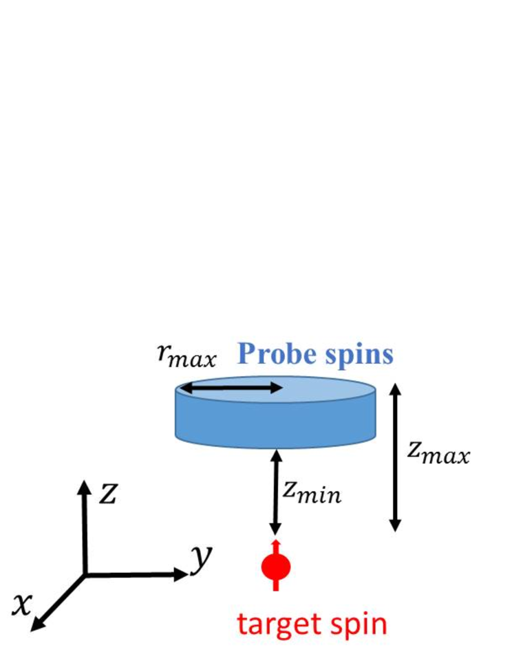
Figure 3: Detection of a target spin with an ensemble of probe spins. Here, we assume that the probe spins are homogeneously distributed inside a columnar form that is placed at a distance from the target spin.

First, we consider a columnar form for the distribution of the probe spins, as shown in Fig. 3. Note that existing technology allows us to fabricate such a structure by combining electron-beam lithography and reactive ion etching, and we can use this structure as the tip for a scanning microscope Maletinsky et al. (2012).

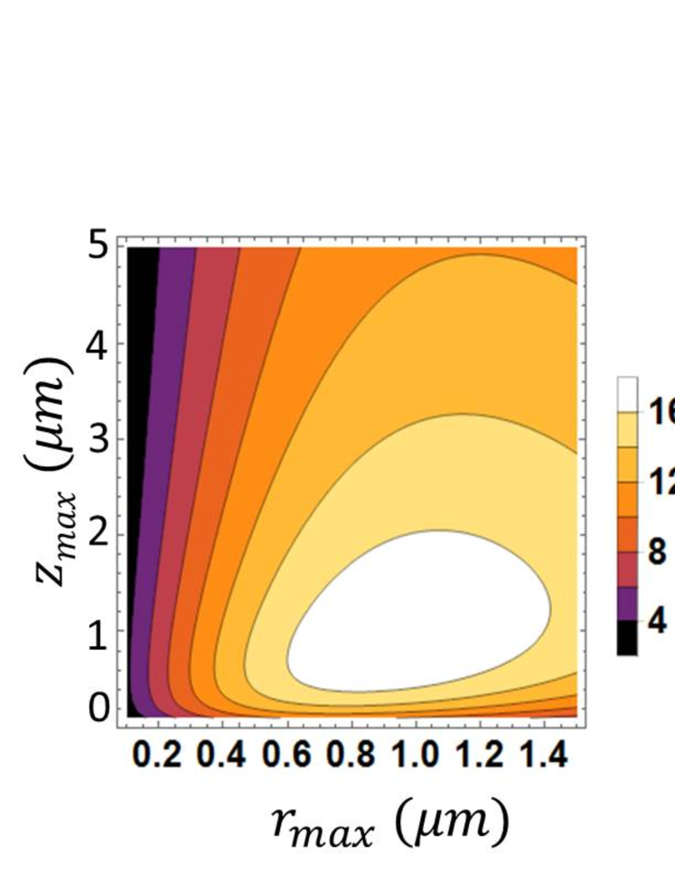
Figure 4: Plot of the ratio $\delta s^{(\rm{single})}_{\rm{min}}/\delta s^{(\rm{ens})}_{\rm{min}}$ with a columnar configuration, as described in Fig. 3. We chose the parameters $T_{2}^{(\rm{single})}=2$ ms for the single probe spin, and $T_{2}^{(\rm{ens})}=84\,\mu$s and $\rho=6.7\times 10^{16}/{\rm{cm}^{3}}$ for the ensemble of the probe spins. In addition, we fixed $z_{\rm{min}}=1\,\mu$m. The ratio shows a maximum value of $\delta s^{(\rm{single})}_{\rm{min}}/\delta s^{(\rm{ens})}_{\rm{min}}\simeq 17.5$ for $r_{\rm{max}}=0.93\,\mu$m and $z_{\rm{max}}=1.87\mu m$.

We can calculate

$$\int_{0}^{r_{\rm{max}}}dr\int_{0}^{2\pi}d\theta\int_{z_{\rm{min}}}^{z_{\rm{max}}}dz\frac{r(\frac{3z^{2}}{r^{2}+z^{2}}-1)}{(r^{2}+z^{2})^{\frac{3}{2}}}$$

$$= 2\pi\Big{(}\frac{z_{\rm{max}}}{\sqrt{r^{2}_{\rm{max}}+z^{2}_{\rm{max}}}}-\frac{z_{\rm{min}}}{\sqrt{r^{2}_{\rm{max}}+z^{2}_{\rm{min}}}}\Big{)}$$

where $\rho$ denotes the density of the probe spin. Therefore, the uncertainty of the estimation is calculated as

$$\delta s^{(\rm{ens})}_{\rm{min}}\simeq\frac{\sqrt{\rho(z_{\rm{max}}-z_{\rm{min}})\pi r^{2}_{\rm{max}}}}{4\pi\rho Ge^{-\frac{1}{2}}\Big{(}\frac{z_{\rm{max}}}{\sqrt{r^{2}_{\rm{max}}+z^{2}_{\rm{max}}}}-\frac{z_{\rm{min}}}{\sqrt{r^{2}_{\rm{max}}+z^{2}_{\rm{min}}}}\Big{)}}\frac{1}{\sqrt{\frac{T_{2}T}{2}}}$$

For comparison, we consider the uncertainty when we use a single probe spin for the spin detection by substituting $x=y=0$ and $z=z_{\rm{min}}$ into Eq. 12.

$$\delta s^{\rm{(single)}}\simeq\frac{1}{e^{-\frac{1}{2}}\frac{4G}{z^{3}_{\rm{min}}}}\frac{1}{\sqrt{\frac{T_{2}T}{2}}}$$ (14)

We can define the ratio of the uncertainty of the estimation as

$$\frac{\delta s^{(\rm{single})}_{\rm{min}}}{\delta s^{(\rm{ens})}_{\rm{min}}}=\frac{\pi\sqrt{\rho}z^{3}_{\rm{min}}\Big{(}\frac{z_{\rm{max}}}{\sqrt{r^{2}_{\rm{max}}+z^{2}_{\rm{max}}}}-\frac{z_{\rm{min}}}{\sqrt{r^{2}_{\rm{max}}+z^{2}_{\rm{min}}}}\Big{)}}{\sqrt{(z_{\rm{max}}-z_{\rm{min}})\pi r^{2}_{\rm{max}}}}\sqrt{\frac{T_{2}^{(\rm{ens})}}{T_{2}^{\rm{(single)}}}}$$

To calculate this ratio, we performed numerical simulations.

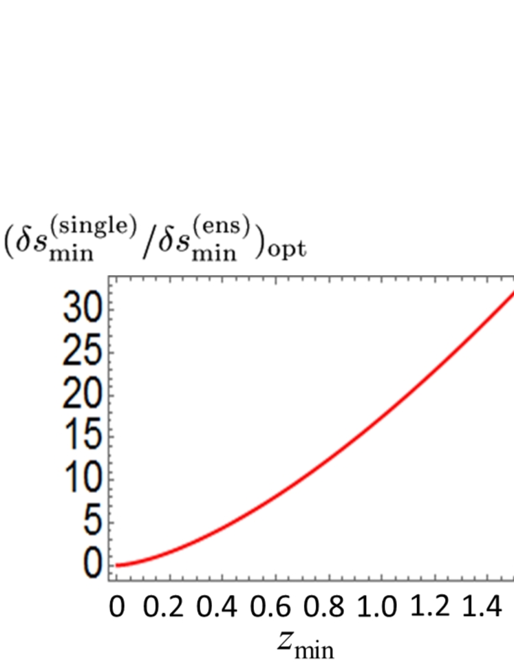
Figure 5: We plot an optimize ratio $\delta s^{(\rm{single})}_{\rm{min}}/\delta s^{(\rm{ens})}_{\rm{min}}$ against $z_{\rm{min}}$ where we choose $r_{\rm{max}}$ and $z_{\rm{max}}$ to maximize this ratio by a continuous line. Except these two parameters, we used the same parameters as the Fig. 4. The ensemble probe spins shows better performance than the single probe spin as long as $z_{\rm{min}}\geq 0.15\mu$m.

For the simulations, we used typical parameters for the nitrogen vacancy (NV) centers in diamond. The NV center is a fascinating candidate for realizing a sensitive magnetic-field sensor Maze et al. (2008); Taylor et al. (2008); Balasubramanian et al. (2008); Schaffry et al. (2011). We can use this system as an effective two-level system, and high fidelity gate operations using microwave pulses have already been demonstrated Davies (1994); Gruber et al. (1997); Jelezko et al. (2002, 2004). Moreover, it is known that we can read out the state of the NV centers via fluorescence from the optical transitions after irradiation with a green laser Gruber et al. (1997); Jelezko et al. (2002). In particular, single NV centers have a long coherence time , e.g., a few milliseconds Balasubramanian et al. (2009); Mizuochi et al. (2009). It is possible to fabricate high-density NV centers , which have been used for magnetic-field sensing Acosta et al. (2009); Maertz et al. (2010); Le Sage et al. (2013); Wolf et al. (2015);however, the coherence time of an ensemble of NV centers is typically much shorter than that of a single NV center. In our numerical simulations, we use values of $T_{2}^{(\rm{single})}=2$ ms for a single NV center and $T_{2}^{(\rm{ens})}=84\,\mu$s and $\rho=6.7\times 10^{16}/{\rm{cm}^{3}}$ for an ensemble of NV centers Balasubramanian et al. (2009); Grezes et al. (2015); Wolf et al. (2015). Note that, even though we focused on NV centers in the numerical simulations, we can, in principle, use other spin ensembles such as donors in high- purity silicon or erbium impurities in yttrium orthosilicate, which can be read out via a superconducting circuit Bushev et al. (2011); Tyryshkin et al. (2012); Tanaka et al. (2015); Toida et al. (2016); Bienfait et al. (2016).

We plot the ratio $\delta s^{(\rm{single})}_{\rm{min}}/\delta s^{(\rm{ens})}_{\rm{min}}$ against $z_{\rm{max}}$ and $r_{\rm{max}}$ in Fig. 4, where we fix $z_{\rm{min}}=1\,\mu$m. There exists an optimal set of $z_{\rm{max}}$ and $r_{\rm{max}}$, and the maximized ratio is approximately $\delta s^{(\rm{single})}_{\rm{min}}/\delta s^{(\rm{ens})}_{\rm{min}}\simeq 17.5$. This means that the ensemble of spins actually shows better performance for spin detection than a single probe spin with these realistic parameters. In addition, we plotted the optimized value of $\delta s^{(\rm{single})}_{\rm{min}}/\delta s^{(\rm{ens})}_{\rm{min}}$ against $z_{\rm{min}}$ in Fig. 5 ,where we chose $z_{\rm{max}}$ and $r_{\rm{max}}$ to maximize $\delta s^{(\rm{single})}_{\rm{min}}/\delta s^{(\rm{ens})}_{\rm{min}}$.The probe-spin ensemble has better sensitivity than the single probe spin as long as $z_{\rm{min}}\geq 0.15\ \mu$m.

III.2 Cylindrical form form for the distribution of probe spins

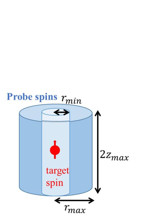
Figure 6: Detection of a target spin with an ensemble of probe spins using a cylindrical form. Here, after fabricating the probe-spin substrate into a columnar form with radius of $r_{\rm{max}}$, we created a hole penetrating the structure with radius $r_{\rm{min}}$. We assume that the probe spins are homogeneously distributed in the substrate and that the target spin is located inside the hole.

Second, we consider a cylindrical form for the distribution of the probe spins, as shown in Fig. 6. After we fabricate a probe-spin substrate (such as diamonds) into a columnar form, we make a hole penetrating the structure.The target spin is located in the center of the hole. Such a fabrication is possible if we use a focused ion beam Hadden et al. (2010). Unlike the columnar form as described in the previous subsection, it is difficult to use this structure with a scanning microscope because the target spin is assumed to be inside the cylindrical form. However, as we will describe, this cylindrical form shows much better performance than the columnar form for spin detections.Therefore, for a proof of principle experiment, this structure would be suitable.

Figure 7: Plot of the $\delta s^{(\rm{single})}_{\rm{min}}/\delta s^{(\rm{ens})}_{\rm{min}}$ with a cylindrical configuration, as described in Fig. 6. We chose the same parameters as in Fig. 7. In addition, we fixed $r_{\rm{min}}=1\,\mu$m. The ratio shows a maximum value of $\delta s^{(\rm{single})}_{\rm{min}}/\delta s^{(\rm{ens})}_{\rm{min}}\simeq 45$ for $r_{\rm{max}}=1.77\,\mu$m and $z_{\rm{max}}=0.58\,\mu m$.

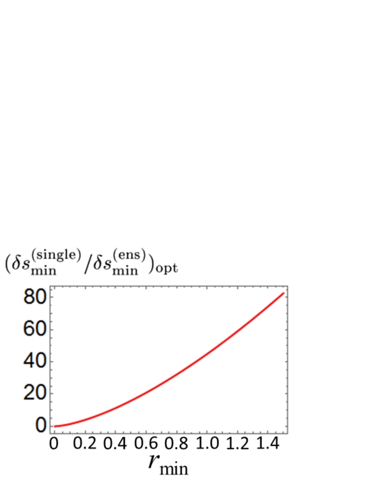
Figure 8: Plot of the optimized ratio $\delta s^{(\rm{single})}_{\rm{min}}/\delta s^{(\rm{ens})}_{\rm{min}}$ versus $r_{\rm{min}}$ where we chose $r_{\rm{max}}$ and $z_{\rm{max}}$ to maximize the ratio. Except for these two parameters, we used the same parameters as the Fig. 7. The ensemble of probe spins shows better performance than the single probe spin as long as $r_{\rm{min}}\geq 0.08\,\mu$m.

We calculated the uncertainty of the estimation as

$$\delta s^{(\rm{ens})}_{\rm{min}}\simeq\frac{e^{\frac{1}{2}}\sqrt{2\rho\pi z_{\rm{max}}(r^{2}_{\rm{max}}-r^{2}_{\rm{min}})}}{|2G\rho\int^{r_{\rm{max}}}_{r_{\rm{min}}}dr\int_{0}^{2\pi}d\theta\int^{z_{\rm{max}}}_{-z_{\rm{max}}}dz\frac{r(\frac{3z^{2}}{r^{2}+z^{2}}-1)}{(r^{2}+z^{2})^{\frac{3}{2}}}\sqrt{\frac{T^{(\rm{ens})}_{2}T}{2}}|}.$$

For comparison, we consider the uncertainty when we use a single probe spin for the spin detection by substituting $x=r_{\rm{min}}$ and $y=z=0$ into Eq. 12.

$$\delta s^{(\rm{single})}_{\rm{min}} \simeq \frac{e^{\frac{1}{2}}(r_{\rm{min}})^{3}}{2G}\frac{1}{\sqrt{\frac{TT^{\rm{(single)}}_{2}}{2}}}.$$

We can define the ratio of the uncertainty of the estimation as

$$\frac{\delta s^{(\rm{single})}_{\rm{min}}}{\delta s^{(\rm{ens})}_{\rm{min}}}=\frac{(r_{\rm{min}})^{3}\sqrt{\frac{T_{2}^{\rm{(ens)}}}{T_{2}^{\rm{(single)}}}}\int^{r_{\rm{max}}}_{r_{\rm{min}}}dr\int^{z_{\rm{max}}}_{-z_{\rm{max}}}dz\frac{r(\frac{3z^{2}}{r^{2}+z^{2}}-1)}{(r^{2}+z^{2})^{\frac{3}{2}}}}{\sqrt{z_{\rm{max}}(r^{2}_{\rm{max}}-r^{2}_{\rm{min}})/(2\pi\rho)}}\ \$$ (15)

We plot the ratio $\delta s^{(\rm{single})}_{\rm{min}}/\delta s^{(\rm{ens})}_{\rm{min}}$ against $z_{\rm{max}}$ and $r_{\rm{max}}$ in Fig. 7, where we fix $r_{\rm{min}}=1\,\mu$m. We have an optimal set of $z_{\rm{max}}$ and $r_{\rm{max}}$. The maximized ratio is approximately $\delta s^{(\rm{single})}_{\rm{min}}/\delta s^{(\rm{ens})}_{\rm{min}}\simeq 45$;therefore, the sensitivity with the ensemble of probe spins is much better than that with the single probe spin. In addition, we conclude that, if we use an ensemble of probe spins, the cylinder configuration shows a better performance for the spin detection than the columnar configuration. Moreover, we plotted the an optimized value of $\delta s^{(\rm{single})}_{\rm{min}}/\delta s^{(\rm{ens})}_{\rm{min}}$ versus $r_{\rm{min}}$ in Fig. 8, where we chose $z_{\rm{max}}$ and $r_{\rm{max}}$ to maximize $\delta s^{(\rm{single})}_{\rm{min}}/\delta s^{(\rm{ens})}_{\rm{min}}$. The probe-spin ensemble in the cylindrical configuration has better sensitivity than the single probe spin as long as $r_{\rm{min}}\geq 0.08\ \mu$m.

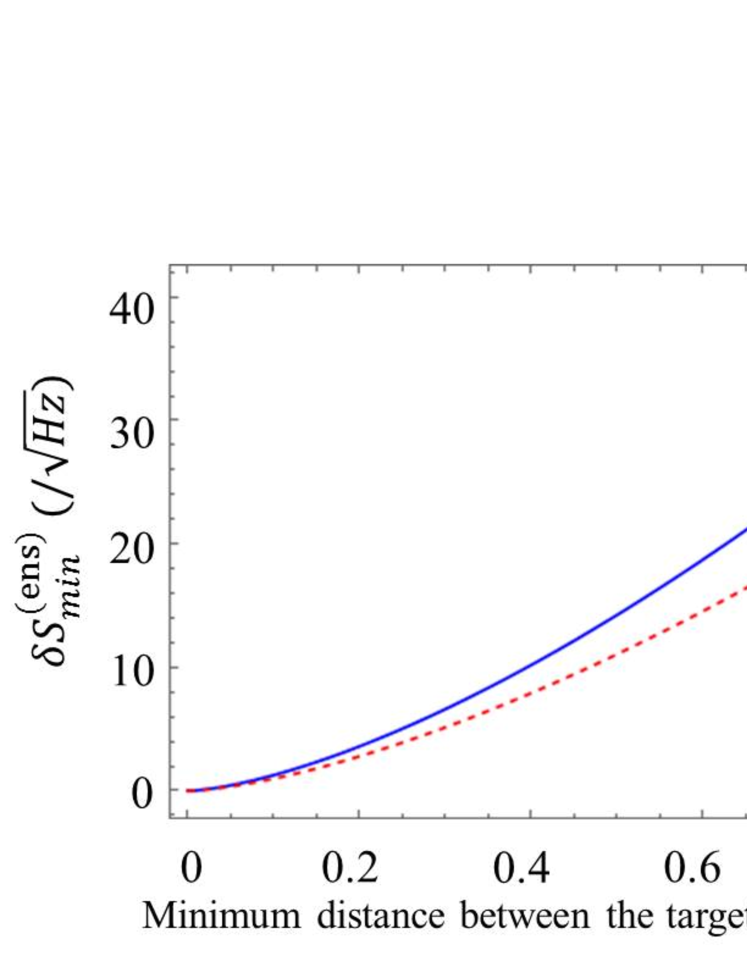
Figure 9: We plot an optimize ratio $\delta s^{(\rm{ens})}_{\rm{min}}$ against $z_{\rm{min}}$ ($r_{\rm{min}}$) to detect a single electron target spin for columnar (cylindrical) distribution of the probe spins by a continuous (dashed) line. Here, we choose $r_{\rm{max}}$ and $z_{\rm{max}}$ to maximize this ratio Except these two parameters, we used the same parameters as the Fig. 7.

Finally, we plotted $\delta s^{(\rm{ens})}_{\rm{min}}$ to estimate the necessary time for the spin detection. We considered an electron spin to be the target spin. As shown in Fig. 9, when the probe spins are distributed in a columnar (cylindrical) form, we obtain $\delta s^{(\rm{ens})}_{\rm{min}}=10$ for $z_{\rm{min}}\simeq 395$nm ($r_{\rm{min}}\simeq 468$nm) when we repeat the experiment for $T=1$ $s$. Since we need to achieve $\delta s^{(\rm{ens})}_{\rm{min}}\simeq 1$ to detect the target spin, the required time for the detection is approximately $T\simeq 100$ $s$. Therefore, when the distance between the target spin and probe spins is of the order of hundreds of nanometers, it takes around a few minutes to detect a single electron spin with the probe spin ensemble in our scheme, which is more than one order of magnitude faster than the case of a single probe spin as shown in Figs. 5 and 8.

IV CONCLUSIONS

We investigated the sensitivity of a single target spin detection using an ensemble of probe spins. The use of a probe spin ensemble increases the signal from the target spin while the projection noise becomes more relevant as we increase the number of probe spins. We demonstrated that, by optimizing the distribution of the probe spins, the signal enhancement of the probe- spin ensemble becomes much larger than the projection noise, which allows us to detect the single target spin much more efficiently than in the case of a single probe spin. In particular, our scheme is useful when the distance between the target spin and the probe spins is of the order of hundreds of nanometers, which makes it difficult for the single probe spin to detect the target due to the weak signal. Our results pave the way for a new strategy to realize reliable single-spin detections.

We thank Sayaka Kitazawa for useful discussions. It was supported by JSPS KAKENHI Grant No. 15K17732. This work was also supported by MEXT KAKENHI Grants No. 15H05868, No. 15H05870, No. 15H03996, No. 26220602 and No. 26249108. The work was also supported by Advanced Photon Science Alliance (APSA), JSPS Core-to-Core Program, and Spin-NRJ.

References

Ramsden (2006)
E. Ramsden,
Hall-effect sensors. newnes (2006).
Vasyukov et al. (2013)
D. Vasyukov,
Y. Anahory,
L. Embon,
D. Halbertal,
J. Cuppens,
L. Neeman,
A. Finkler,
Y. Segev,
Y. Myasoedov,
M. L. Rappaport,
et al., Nature nanotechnology
8, 639 (2013).
Bal et al. (2012)
M. Bal,
C. Deng,
J. Orgiazzi,
F. Ong, and
A. Lupascu,
Nature Communications 3,
1324 (2012).
Toida et al. (2016)
H. Toida,
Y. Matsuzaki,
K. Kakuyanagi,
X. Zhu,
W. J. Munro,
K. Nemoto,
H. Yamaguchi,
and S. Saito,
Applied Physics Letters 108,
052601 (2016).
Bienfait et al. (2016)
A. Bienfait,
J. Pla,
Y. Kubo,
M. Stern,
X. Zhou,
C. Lo,
C. Weis,
T. Schenkel,
M. Thewalt,
D. Vion, et al.,
Nature nanotechnology 11,
253 (2016).
Rugar et al. (2004)
D. Rugar,
R. Budakian,
H. Mamin, and
B. Chui,
Nature 430,
329 (2004).
Degen (2008)
C. Degen,
Nature nanotechnology 3,
643 (2008).
Maze et al. (2008)
J. Maze,
P. Stanwix,
J. Hodges,
S. Hong,
J. Taylor,
P. Cappellaro,
L. Jiang,
M. Dutt,
E. Togan,
A. Zibrov,
et al., Nature
455, 644 (2008),
ISSN 0028-0836.
Taylor et al. (2008)
J. Taylor,
P. Cappellaro,
L. Childress,
L. Jiang,
D. Budker,
P. Hemmer,
A. Yacoby,
R. Walsworth,
and M. Lukin,
Nature Physics 4,
810 (2008).
Balasubramanian
et al. (2008)
G. Balasubramanian,
I. Chan,
R. Kolesov,
M. Al-Hmoud,
J. Tisler,
C. Shin,
C. Kim,
A. Wojcik,
P. Hemmer,
A. Krueger,
et al., Nature
455, 648 (2008).
Schaffry et al. (2011)
M. Schaffry,
E. Gauger,
J. Morton, and
S. Benjamin,
Phys. Rev. Lett. 107,
207210 (2011).
Müller et al. (2014)
C. Müller,
X. Kong,
J.-M. Cai,
K. Melentijević,
A. Stacey,
M. Markham,
D. Twitchen,
J. Isoya,
S. Pezzagna,
J. Meijer,
et al., Nature communications
5 (2014).
Staudacher et al. (2013)
T. Staudacher,
F. Shi,
S. Pezzagna,
J. Meijer,
J. Du,
C. A. Meriles,
F. Reinhard, and
J. Wrachtrup,
Science 339,
561 (2013).
Mamin et al. (2013)
H. Mamin,
M. Kim,
M. Sherwood,
C. Rettner,
K. Ohno,
D. Awschalom,
and D. Rugar,
Science 339,
557 (2013).
Ohashi et al. (2013)
K. Ohashi,
T. Rosskopf,
H. Watanabe,
M. Loretz,
Y. Tao,
R. Hauert,
S. Tomizawa,
T. Ishikawa,
J. Ishi-Hayase,
S. Shikata,
et al., Nano letters
13, 4733 (2013).
Rugar et al. (2015)
D. Rugar,
H. Mamin,
M. Sherwood,
M. Kim,
C. Rettner,
K. Ohno, and
D. Awschalom,
Nature nanotechnology 10,
120 (2015).
Vengalattore et al. (2007)
M. Vengalattore,
J. Higbie,
S. Leslie,
J. Guzman,
L. Sadler, and
D. Stamper-Kurn,
Physical review letters 98,
200801 (2007).
Kominis et al. (2003)
I. Kominis,
T. Kornack,
J. Allred, and
M. Romalis,
Nature 422,
596 (2003).
Acosta et al. (2009)
V. Acosta,
E. Bauch,
M. Ledbetter,
C. Santori,
K.-M. Fu,
P. Barclay,
R. Beausoleil,
H. Linget,
J. Roch,
F. Treussart,
et al., Physical Review B
80, 115202
(2009).
Maertz et al. (2010)
B. Maertz,
A. Wijnheijmer,
G. Fuchs,
M. Nowakowski,
and
D. Awschalom,
Applied Physics Letters 96,
092504 (2010).
Le Sage et al. (2013)
D. Le Sage,
K. Arai,
D. Glenn,
S. DeVience,
L. Pham,
L. Rahn-Lee,
M. Lukin,
A. Yacoby,
A. Komeili, and
R. Walsworth,
Nature 496,
486 (2013).
Wolf et al. (2015)
T. Wolf,
P. Neumann,
K. Nakamura,
H. Sumiya,
T. Ohshima,
J. Isoya, and
J. Wrachtrup,
Physical Review X 5,
041001 (2015).
Dolde et al. (2011)
F. Dolde,
H. Fedder,
M. Doherty,
T. Nöbauer,
F. Rempp,
G. Balasubramanian,
T. Wolf,
F. Reinhard,
L. Hollenberg,
F. Jelezko,
et al., Nature Physics
7, 459 (2011).
De Lange et al. (2010)
G. De Lange,
Z. Wang,
D. Riste,
V. Dobrovitski,
and R. Hanson,
Science 330,
60 (2010).
Maletinsky et al. (2012)
P. Maletinsky,
S. Hong,
M. Grinolds,
B. Hausmann,
M. Lukin,
R. Walsworth,
M. Loncar, and
A. Yacoby,
Nature Nanotechnology 7,
320 (2012).
Davies (1994)
G. Davies,
Properties and Growth of Diamond
(Inspec/Iee, 1994).
Gruber et al. (1997)
A. Gruber,
A. Dräbenstedt,
C. Tietz,
L. Fleury,
J. Wrachtrup,
and
C. Von Borczyskowski,
Science 276,
2012 (1997).
Jelezko et al. (2002)
F. Jelezko,
I. Popa,
A. Gruber,
C. Tietz,
J. Wrachtrup,
A. Nizovtsev,
and S. Kilin,
Appl. Phys. Lett. 81,
2160 (2002).
Jelezko et al. (2004)
F. Jelezko,
T. Gaebel,
I. Popa,
A. Gruber, and
J. Wrachtrup,
Phys. Rev. Lett 92,
076401 (2004).
Balasubramanian
et al. (2009)
G. Balasubramanian,
P. Neumann,
D. Twitchen,
M. Markham,
R. Kolesov,
N. Mizuochi,
J. Isoya,
J. Achard,
J. Beck,
J. Tissler,
et al., Nature materials
8, 383 (2009).
Mizuochi et al. (2009)
N. Mizuochi,
P. Neumann,
F. Rempp,
J. Beck,
V. Jacques,
P. Siyushev,
K. Nakamura,
D. Twitchen,
H. Watanabe,
S. Yamasaki,
et al., Physical review B
80, 041201
(2009).
Grezes et al. (2015)
C. Grezes,
B. Julsgaard,
Y. Kubo,
W. Ma,
M. Stern,
A. Bienfait,
K. Nakamura,
J. Isoya,
S. Onoda,
T. Ohshima,
et al., Physical Review A
92, 020301
(2015).
Bushev et al. (2011)
P. Bushev,
A. Feofanov,
H. Rotzinger,
I. Protopopov,
J. Cole,
C. Wilson,
G. Fischer,
A. Lukashenko,
and A. Ustinov,
Physical Review B 84,
060501 (2011).
Tyryshkin et al. (2012)
A. M. Tyryshkin,
S. Tojo,
J. J. Morton,
H. Riemann,
N. V. Abrosimov,
P. Becker,
H.-J. Pohl,
T. Schenkel,
M. L. Thewalt,
K. M. Itoh,
et al., Nature materials
11, 143 (2012).
Tanaka et al. (2015)
T. Tanaka,
P. Knott,
Y. Matsuzaki,
S. Dooley,
H. Yamaguchi,
W. J. Munro, and
S. Saito,
Phys. Rev. Lett. 115,
170801 (2015).
Hadden et al. (2010)
J. Hadden,
J. Harrison,
A. Stanley-Clarke,
L. Marseglia,
Y.-L. Ho,
B. Patton,
J. O Brien, and
J. Rarity,
Applied Physics Letters 97,
241901 (2010).