Beam Dynamics Analysis of Dielectric Laser Acceleration using a Fast 6D Tracking Scheme

Abstract

A six-dimensional symplectic tracking approach exploiting the periodicity properties of Dielectric Laser Acceleration (DLA) gratings is presented. The longitudinal kick is obtained from the spatial Fourier harmonics of the laser field within the structure, and the transverse kicks are obtained using the Panofsky-Wenzel theorem. Additionally to the usual, strictly longitudinally periodic gratings, our approach is also applicable to periodicity chirped (sub-relativistic) and tilted (deflection) gratings. In the limit of small kicks and short periods we obtain the 6D Hamiltonian, which allows, for example, to obtain matched beam distributions in DLAs. The scheme is applied to beam and grating parameters similar to recently performed experiments. The paper concludes with an outlook to laser based focusing schemes, which are promising to overcome fundamental interaction length limitations, in order to build an entire microchip-sized laser driven accelerator.

I Introduction

Dielectric Laser Acceleration (DLA) provides highest gradients among non-plasma accelerators. In 2013, the acceleration of relativistic electrons was demonstrated at SLAC with a gradient of more than 250 MeV/m Peralta et al. (2013), which was recently increased to 690 MeV/m Wootton et al. (2016a). Low energy electrons (27.7 keV) were accelerated by the group in Erlangen Breuer and Hommelhoff (2013) with a gradient of 25 MeV/m using a single grating structure. The group at Stanford University used a dual pillar structure to accelerate 96 keV electrons with a gradient of more than 200 MeV/m Leedle et al. (2015). In principle, the gradient of a DLA is only limited by the structure damage threshold fluence, which is roughly two orders of magnitude higher for dielectrics than for metals. The reason for the rediscovery of this rather old concept of inverse Smith-Purcell or inverse Cherenkov effects for particle acceleration (see e.g. Shimoda (1962)) is that nowadays both the ultrashort laser pulse control techniques as well as the nano-fabrication have significantly improved. Summaries of the recent developments can be found in England et al. (2014) and Wootton et al. (2016b).

Although the experimentally demonstrated gradients in DLA structures are very promising, there are still crucial challenges to create a miniaturized DLA-based particle accelerator. So far the experimentally achieved gradients could only be used to increase the beam’s energy spread and not for coherent acceleration. Moreover, the interaction length with present DLA structures is limited to the Rayleigh range (see App. A) of the incident electron beam. For low energy electrons, due to the high gradient, the acceleration defocusing even leads to interaction distances significantly shorter than the Rayleigh range.

Thus, in order to use DLA for a real accelerator, focusing schemes have to be developed. One option would be Alternating Phase Focusing (APF) as outlined in Fig. 1. Here, drift sections between grating cells lead to jumps in the synchronous phase, which can be designed to provide net focusing. Such schemes can be a way to increase the interaction length in DLAs and make an accelerator on a microchip feasible.

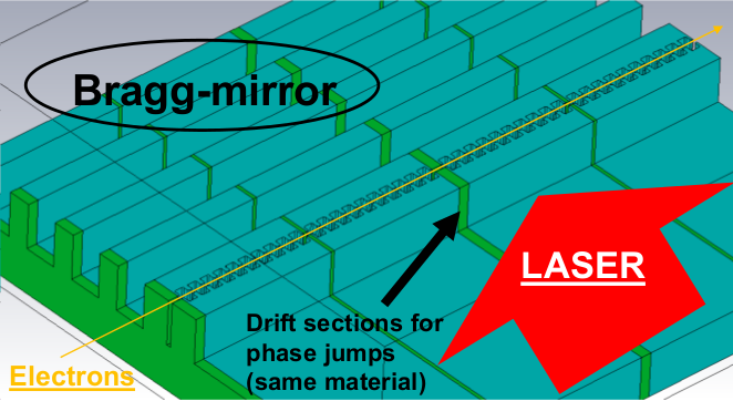
Figure 1: Example Bragg cavity grating with a Bragg mirror on one side.

A challenge in the creation of a DLA based optical accelerator is related to the complex 3D beam dynamics in DLA structures, which has not been treated systematically in the existing literature yet. In order to facilitate front to end simulations and identify optimized DLA structures, we employ a simple and efficient numerical tracking scheme, which does not require a large amount of computing power, it runs in Matlab MathWorks (2016) on an ordinary PC.

Due to the periodicity of a DLA grating, only one spatial Fourier harmonic contributes to the kick of the beam. In a simplified approach, where fringe fields are neglected, the entire laser field can be represented by a set of such Fourier coefficients, where only one complex number represents each grating cell. By means of the Panofsky-Wenzel theorem Panofsky and Wenzel (1956), this single complex number also allows to determine the transverse kicks experienced by a particle while traveling through one grating period.

When the three-dimensional kicks are applied to the beam particles in a symplectic scheme (we use symplectic Euler, which is equivalent to Leap Frog) the tracking becomes phase space volume preserving. Thus, with no numerical (artificial) emittance increase, the physical emittance increase due to the nonlinear fields in the DLA interaction can be calculated. Moreover, since the equations of motion are coupled, there is also emittance exchange between the different planes which can be analyzed.

In the present study we neglect all intensity dependent effects as space charge, wakes, and radiation emission. The number of particles is chosen such that smooth spectra are obtained, a reasonable value is $10^{6}$, at which the computational time is about one second per grating cell.

With no loss of generality, we restrict ourselves to symmetric grating structures driven from both lateral sides. This makes sure that the axis of symmetry is in the center and the fields have a $\cosh$ profile. In the case of non-symmetric structures or non-symmetric driving the fields will have an exponential or an off-axis $\cosh$ profile. However, single driver systems can be combined with Bragg mirrors in order to obtain a good approximation to an on-axis $\cosh$ profile with a single side driver (see again Fig. 1).

As it is usually done e.g. for the synchrotron motion in ion synchrotrons, we take the limit from the tracking difference equations to differential equations. Since the three-dimensional kick must be irrotational due to the Panofsky-Wenzel theorem, it can be derived from a scalar potential. This potential directly allows to determine the 6D Hamiltonian which completely describes the single particle dynamics analytically.

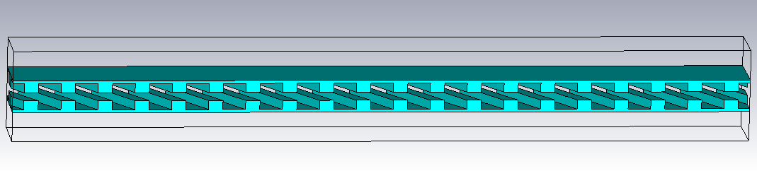
Figure 2: Tilted Bragg cavity grating, where the dual drive laser comes from top and bottom and is polarized in the electron beam direction (left to right).

Both the numerical and the analytical approach can be generalized from ordinary DLA gratings to tilted DLA gratings, which have been proposed as deflectors or laser driven undulators Plettner and Byer (2008a, b); Plettner et al. (2009). Such a grating is depicted in Fig. 2. However, since our code does not include the radiation fields, a dedicated code as e.g. Fallahi et al. (2016) can be used to treat the dynamics self consistently. The analytical kicks reported here can serve as input quantities. Our approach aims at maximal simplicity such that studies of fundamental questions, as e.g. transverse focusing and deflection, are quickly possible.

The paper is organized as follows. Section II presents the determination of the longitudinal and transverse fields and kicks in a single grating period. Here we use CST Studio Suite CST (2016) to calculate the longitudinal kick at the center of the structure. The dependence on the transverse coordinates as well as the transverse kicks are modeled analytically. In Sect. III we present a symplectic 6D tracking method based on one kick per grating period. Analytical descriptions of the coupled longitudinal and transverse beam dynamics as well as the full 6D Hamiltonian are given in Sect. IV. Simplifications and beam matching in linearized fields are also discussed in this section. In Sect. V we address the three crucial examples: subrelativistic acceleration, relativistic acceleration, and deflection by means of DLA gratings. The paper concludes with a summary and an outlook to DLA focusing channels in Sect. VI.

II Fields and kicks in periodic structures

Usual particle tracking algorithms solve Maxwell’s equations with a predefined time step. Instead of that, we make use of the periodicity of the structure and apply only the kicks which are known not to average out a-priori. The other field harmonics are neglected. The validity of this neglect depends on the effect of transients which is effectively suppressed when the structure period is matched to the beam velocity. With no loss of generality we restrict ourselves here to an infrared laser with $\lambda_{0}=1.96\;\mu$m and structures made of Silicon ($\varepsilon_{r}=11.63$). A single cell of a symmetrically driven Bragg mirror cavity structure is shown in Fig. 3.

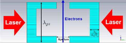
Figure 3: One period of a symmetric Bragg mirror cavity structure.

II.1 Analysis of the longitudinal field

A coordinate system is applied such that the electron beam propagates in positive z-direction and the z-polarized laser propagates in y-direction. The unit cell of a periodic dielectric structure has dimensions $\lambda_{gx}$ and $\lambda_{gz}$. In order to allow the laser field to escape the structure, open boundaries in positive and negative y-direction are assumed.

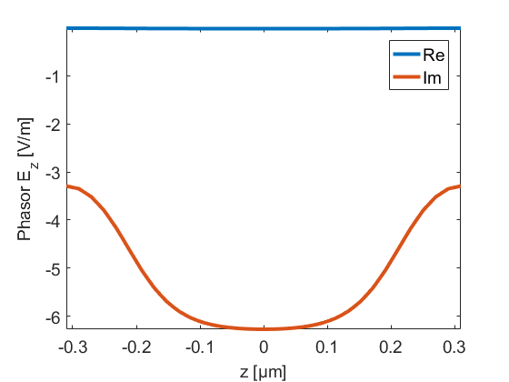
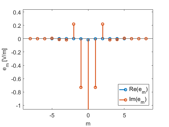
Figure 4: Longitudinal electric field on the beam axis for the Bragg mirror structure in Fig. 3 and spatial Fourier harmonics for incident laser field normalized to 1 V/m.

The energy gain of a particle in one cell is

$$\Delta W(x,y;s) =q\int\limits_{-\lambda_{gz}/2}^{\lambda_{gz}/2}E_{z}(x,y,z;t=(z+s)/v)\mathrm{d}z$$ (1)

$$=q\int\limits_{-\lambda_{gz}/2}^{\lambda_{gz}/2}{\rm Re}\,\{\underline{E}_{z}(x,y,z)e^{i\omega(z+s)/v}\}\mathrm{d}z,$$ (2)

where the underlined electric field is a phasor at the fixed frequency $\omega=2\pi c/\lambda_{0}$ of the laser, and $q$ is the charge ($q=-e$ for electrons). The variable $s$ denotes the relative position of the particle behind an arbitrarily defined reference particle moving at $z=vt$. Thus $z$ is the absolute position in the laboratory frame, while $s$ denotes the phase shift w.r.t. $z$. Due to the $z$-periodicity, the laser field can be expanded in spatial Fourier series

$$\underline{E}_{z}(x,y,z) =\sum\limits_{m=-\infty}^{\infty}\underline{e}_{m}(x,y)e^{-im\frac{2\pi}{\lambda_{gz}}z}$$ (3)

$$\underline{e}_{m}(x,y) =\frac{1}{\lambda_{gz}}\int\limits_{-\lambda_{gz}/2}^{\lambda_{gz}/2}\underline{E}_{z}(x,y,z)e^{im\frac{2\pi}{\lambda_{gz}}z}\mathrm{d}z,$$ (4)

which allows to compute the energy gain integral (Eq. 2) as

$$\Delta W(x,y;s)=q{\rm Re}\,\left\{e^{2\pi i\frac{s}{\beta\lambda_{0}}}\sum\limits_{m=-\infty}^{\infty}\underline{e}_{m}(x,y)\lambda_{gz}\mathrm{sinc}\left[\pi\left(\frac{\lambda_{gz}}{\beta\lambda_{0}}-m\right)\right]\right\}.$$ (5)

The electric field phasor and its spatial Fourier coefficients for the structure in Fig. 3 are plotted in Fig. 4. It has a small real part, which is coincidental, and a strong first and weak second harmonic. If the round braces in Eq. 5 is non-integer, the energy gain averages to zero, if it is integer other than zero, it directly vanishes. Thus we have the phase synchronicity condition

$$\lambda_{gz}=m\beta\lambda_{0}$$ (6)

and the particle’s energy gain simplifies to

$$\Delta W(x,y;s)=q\lambda_{gz}{\rm Re}\,\left\{e^{2\pi i\frac{s}{\beta\lambda_{0}}}\underline{e}_{m}(x,y)\right\}=q\lambda_{gz}|\underline{e}_{m}|\cos\left(2\pi\frac{s}{\beta\lambda_{0}}+\varphi_{m}\right),$$ (7)

where $\varphi_{m}=\arctan{\rm Im}\,\{\underline{e}_{m}\}/{\rm Re}\,\{\underline{e}_{m}\}$ is the phase of the Fourier coefficient. The energy gain is maximal at $s_{opt}=-\varphi_{m}\beta\lambda_{0}/2\pi$ for positively charged particles and $s_{opt}=-(\varphi_{m}+\pi)\beta\lambda_{0}/2\pi$ for electrons. Zero acceleration is found at $s_{0}=-(\varphi_{m}\pm\pi/2)\beta\lambda_{0}/2\pi$, where all these expressions are to be taken modulo $\beta\lambda_{0}/m$. The integer spatial harmonic $m$ has the same meaning as the harmonic number in conventional accelerators, i.e. the number of buckets per grating period and Eq. 6 resembles the Wideroe condition. The non-synchronous harmonics, which we assume to average out in this framework, however provide kicks in the case $s$ in Eq. 5 is not a constant. This leads then to multi-harmonic buckets and can also be used for ponderomotive focusing, see Naranjo et al. (2012).

For sub-relativistic accelerators, the grating needs to be chirped in period length in order to always fulfill Eq. 6 on the energy ramp. The change of period length is given by the energy velocity differential

$$\frac{\Delta z}{\lambda_{gz}}=\frac{1}{\beta^{2}\gamma^{2}}\frac{\Delta W}{W}$$ (8)

and is in the range of $\lesssim 1\%$ for $W_{\mathrm{kin}}=30$ keV and $\Delta W/\lambda_{gz}=1$ GeV/m. The thus created ”quasi-periodic” gratings can be seen in good approximation as periodic, however, phase drifts have to be compensated in the structure design Niedermayer et al. (2017).

II.2 Analysis of the transverse field

The transverse field probed by a rigidly moving charge can be obtained using the Panofsky-Wenzel theorem Panofsky and Wenzel (1956), which holds for either vanishing fields at infinity or periodic boundary conditions as

$$\nabla^{\prime}\times\Delta\vec{p}(\vec{r}_{\perp},s)=\int\limits_{-T/2}^{T/2}\mathrm{d}t\left[\nabla\times\vec{F}(\vec{r}_{\perp},z,t)\right]_{z=vt-s}=\left.\vec{B}\right|_{-T/2}^{T/2}=0.$$ (9)

Here the ’relative gradient’ is defined as $\nabla^{\prime}=(\partial_{x},\partial_{y},-\partial_{s})^{\mathrm{T}}$ and $\lambda_{gz}=\beta cT$. The transverse kick per cell can be written as

$$\Delta\vec{p}_{\perp}(x,y;s) =-\int\mathrm{d}s\nabla\!_{\perp}\Delta p_{\parallel}(x,y;s)$$ (10)

$$=-\frac{\lambda_{gz}}{2\pi m}q\frac{1}{\beta c}\nabla\!_{\perp}\int\limits_{-\lambda_{gz}/2}^{\lambda_{gz}/2}{\rm Im}\,\{\underline{E}_{z}(x,y,z)e^{i\omega(z+s)/v}\}\mathrm{d}z,$$ (11)

where the energy momentum differential $\Delta p_{\parallel}=\Delta W/(\beta c)$ was applied. Moreover, if the phase-synchronicity condition (Eq. 6) is fulfilled, the kick becomes

$$\Delta\vec{p}_{\perp}(x,y;s) =-\frac{\lambda_{gz}^{2}}{2\pi m}q\frac{1}{\beta c}\nabla\!_{\perp}{\rm Im}\,\left\{e^{2\pi i\frac{s}{\beta\lambda_{0}}}\underline{e}_{m}(x,y)\right\}$$ (12)

$$=-\frac{\lambda_{gz}}{m}q\frac{1}{\beta c}{\rm Im}\,\left\{e^{2\pi i\frac{s}{\beta\lambda_{0}}}\underline{\vec{f}}_{m}(x,y)\right\},$$ (13)

where $\underline{\vec{f}}_{m}(x,y)=\lambda_{gz}\nabla\!_{\perp}\underline{e}_{m}(x,y)/2\pi$. In the following, the structure under investigation is generalized to a tilted grating as visible in Fig. 5, which reproduces the ordinary grating for tilt angle $\alpha=0$. The tilted grating is periodic in $z$ and $x$ direction. Thus for any function $F(x,y,s)$ must hold

$$\frac{\partial F}{\partial x}=\frac{\partial F}{\partial s}\frac{\partial s}{\partial z}\frac{\partial z}{\partial x}=\frac{\partial F}{\partial s}\tan\alpha.$$ (14)

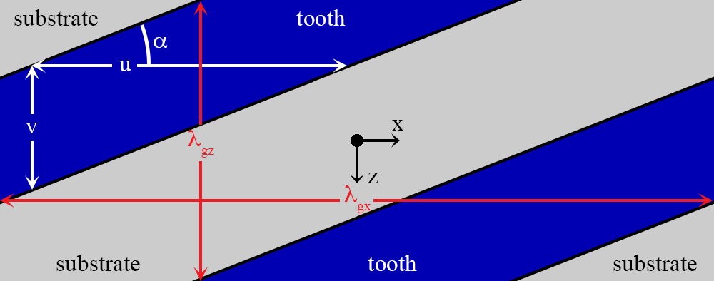
Figure 5: Tilted grating with periodic boundary conditions in $x$ and $z$ direction and $\tan\alpha=\lambda_{\mathrm{gz}}/\lambda_{\mathrm{gx}}=v/u$.

The $s$-derivative can be calculated in the Fourier representation by Eq. 7 as

$$\frac{\partial\underline{e}_{m}(x,y)}{\partial x}=\tan\alpha\frac{2\pi i}{\beta\lambda_{0}}\underline{e}_{m}(x,y).$$ (15)

The derivatives in $y$-direction can be determined by the dispersion relation for the synchronous mode. We have

$$k_{z}=\frac{\omega}{\beta c},\;\;\;k_{x}=\frac{2\pi}{\beta\lambda_{0}}\tan\alpha\;\;\;\mathrm{and}\;\;\;k=\frac{\omega}{c}$$ (16)

and thus

$$k_{y}=\pm\sqrt{k^{2}-(k_{z}^{2}+k_{x}^{2})}=\pm\frac{\omega}{c}\sqrt{1-\frac{1}{\beta^{2}}(1+\tan^{2}\alpha)}.$$ (17)

For a non-tilt grating ($\alpha=0$) this is the well known evanescent decay of the near field $k_{y}=i\omega/(\beta\gamma c)$. Once $k_{x},k_{y}$ are determined, the fields can be found from

$$\underline{e}_{m}(x,y)=\underline{e}_{m}(0,0)\cosh(ik_{y}y)e^{ik_{x}x},$$ (18)

where $\lambda_{gx}=\lambda_{gz}/\tan\alpha$.

A map of the energy gain and transverse kicks for the grating in Fig. 6 can be seen in Fig. 7 for a grating tilt angle $\alpha=30\deg$.

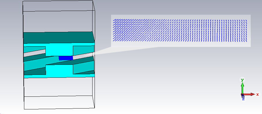
Figure 6: Single cell of the tilted grating deflector structure and enlargement of kick integration curves array. The integrated kicks are displayed in Fig. 7.

The results labeled numerical are obtained by line integration (Eq. 7) of the electric field simulated with CST MWS CST (2016) and the analytical results correspond to Eq. 18.

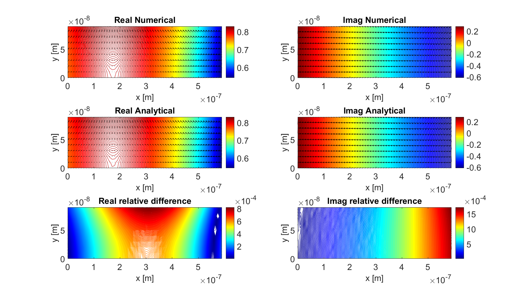
Figure 7: Contour lines of $\underline{e}_{1}(x,y)$ and kick field $\underline{\vec{f}}_{1}(x,y)$ for the tilted grating with $\alpha=30\deg$. The fields have been obtained both analytically and numerically, the bottom plots show the relative difference.

The transverse kicks are obtained by Eq. 13 as

$$\underline{\vec{f}}_{m}(x,y)=\; \underline{e}_{m}(0,0)\cosh(ik_{y}y)e^{ik_{x}x}im\tan\alpha\vec{e}_{x}$$

$$+ \underline{e}_{m}(0,0)\sinh(ik_{y}y)e^{ik_{x}x}(ik_{y}\lambda_{gz}/2\pi)\vec{e}_{y}$$ (19)

and are depicted as arrows in Fig. 7. For the numerical results, the gradient is determined by finite differences in Matlab MathWorks (2016). Note that $-ik_{y}\in\mathbb{R}^{+}$, i.e. the kick in $x$-direction is in phase with the acceleration while the kick in $y$-direction is $90$ degrees shifted.

For a particle that is only slightly displaced from the beam axis by $\Delta\vec{x}=(\Delta x,\Delta y)$ the kick can be written as two-dimensional Taylor expansion

$$\underline{\vec{f}}_{m}(x,y) =\underline{\vec{f}}_{m}(x_{0},y_{0})+(\nabla\!_{\perp}\underline{\vec{f}}_{m}(x_{0},y_{0}))\Delta\vec{x}+\mathcal{O}(||\Delta\vec{x}||^{2})$$

$$=\frac{\lambda_{gz}}{2\pi}\left(\nabla\!_{\perp}\underline{e}_{m}(x_{0},y_{0})+(\nabla\!_{\perp}\nabla\!_{\perp}^{\mathrm{T}})\underline{e}_{m}(x_{0},y_{0})\Delta\vec{x}\right)+\mathcal{O}(||\Delta\vec{x}||^{2}),$$ (20)

where

$$\nabla\!_{\perp}\nabla\!_{\perp}^{\mathrm{T}}=\begin{pmatrix}\partial_{x}^{2}&\partial_{x}\partial_{y}\\ \partial_{y}\partial_{x}&\partial_{y}^{2}\end{pmatrix}$$ (21)

is the Hessian. The expansion Eq. 20 about $x_{0}=0,y_{0}=0$ of Eq. 18 results in

$$\underline{\vec{f}}_{m}(\Delta x,\Delta y)=\dfrac{\lambda_{gz}}{2\pi}\underline{e}_{m}(0,0)\begin{pmatrix}ik_{x}-k_{x}^{2}\Delta x\\ -k_{y}^{2}\Delta y\end{pmatrix},$$ (22)

i.e. a position independent (coherent) kick component in $x$-direction, vanishing for ${\alpha=0}$. Using this abstract derivation, the results of several papers proposing DLA undulators Plettner and Byer (2008a, b); Plettner et al. (2009) can be recovered.

III Tracking equations

In order to study the motion of particles in the fields of periodic gratings we approximate the forces by one kick per grating period and track with the symplectic Euler method. In spite of the very high gradients in DLA structures, the energy can still be seen as an adiabatic variable, as it is the case in conventional linacs. Tracking the full time dependence of $\gamma$, as required for example in plasma accelerators, can be avoided due to the shortness of the periods. For simplicity, we restrict ourselves to $m=1$ from this point and introduce normalized variables in the paraxial approximation

$$x^{\prime}=\frac{p_{x}}{p_{z0}}\;,\;\;\;\Delta x^{\prime}=\frac{\Delta p_{x}(x,y,\varphi)}{p_{z0}}\;,\;\;\;y^{\prime}=\frac{p_{y}}{p_{z0}}\;,\;\;\;\Delta y^{\prime}=\frac{\Delta p_{y}(x,y,\varphi)}{p_{z0}},$$

$$\varphi=2\pi\frac{s}{\lambda_{gz}}\;,\;\;\;\delta=\frac{W-W_{0}}{W_{0}}\;,\;\;\;\Delta\delta=\frac{\Delta W(x,y,\varphi)-\Delta W(0,0,\varphi_{\mathrm{s}})}{W_{0}},$$ (23)

where $W_{0}=\gamma m_{e}c^{2}$ and $p_{z0}=\beta\gamma m_{e}c$. The particle at the synchronous phase $\varphi_{\mathrm{s}}$ has $\Delta\delta=0$, i.e. its energy gain is entirely described by the acceleration ramp. The energy gain $\Delta W$ is given by Eq. 7 and thus the energy gain of the synchronous particle is

$$\Delta W(0,0,\varphi_{\mathrm{s}})=q\lambda_{gz}{\rm Re}\,\left\{e^{i\varphi_{\mathrm{s}}}\underline{e}_{1}\right\},$$ (24)

where we write $\underline{e}_{1}=\underline{e}_{1}(x=0,y=0)$ for brevity. Note that the synchronous phase and the phase of each particle always refer to the laser phase. The sum of the kicks

$$W(N)=W_{\mathrm{init}}+\sum_{n=1}^{N}\Delta W^{(n)}(0,0,\varphi_{\mathrm{s}}^{(n)})$$ (25)

describes the acceleration ramp, where the synchronous phase $\varphi_{\mathrm{s}}$ can be chosen arbitrarily in each grating cell. The variables $e_{1}$, $\lambda_{gz}$, $W_{0}$, $\beta$, $\gamma$, $\varphi_{\mathrm{s}}$ and all variables in Eq. 23 are stored as arrays indexed by the grating cell number. The kicks are obtained using Eqs. 7, 18, 19, and 13 and read

$$\Delta x^{\prime} =-\frac{q\lambda_{0}}{p_{z0}c}\tan(\alpha)\cosh(ik_{y}y){\rm Re}\,\left\{\underline{e}_{1}e^{i\varphi+i\frac{2\pi x}{\lambda_{gx}}}\right\}$$ (26a)

$$\Delta y^{\prime} =\frac{-ik_{y}\lambda_{0}^{2}q\beta}{2\pi p_{z0}c}\sinh(ik_{y}y){\rm Im}\,\left\{\underline{e}_{1}e^{i\varphi+i\frac{2\pi x}{\lambda_{gx}}}\right\}$$ (26b)

$$\Delta\delta =\frac{q\lambda_{gz}}{\gamma m_{e}c^{2}}{\rm Re}\,\left\{\underline{e}_{1}\left(\cosh(ik_{y}y)e^{i\varphi+i\frac{2\pi x}{\lambda_{gx}}}-e^{i\varphi_{s}}\right)\right\},$$ (26c)

where $k_{y}$ is given by Eq. 17. The tracking equations are

$$\left(\begin{array}[]{c}x\\ x^{\prime}\\ y\\ y^{\prime}\\ \varphi\\ \delta\\ \end{array}\right)^{(n+1)}=\left(\begin{array}[]{c}x\\ Ax^{\prime}+\Delta x^{\prime}(x,y,\varphi)\\ y\\ Ay^{\prime}+\Delta y^{\prime}(x,y,\varphi)\\ \varphi\\ \delta+\Delta\delta(x,y,\varphi;\varphi_{\mathrm{sync}})\\ \end{array}\right)^{(n)}+\left(\begin{array}[]{c}\lambda_{gz}x^{\prime}(x,y,\varphi)\\ 0\\ \lambda_{gz}y^{\prime}(x,y,\varphi)\\ 0\\ -\frac{2\pi}{\beta^{2}\gamma^{2}}\delta(x,y,\varphi)\\ 0\\ \end{array}\right)^{(n+1)},$$ (27)

where an explicit scheme is obtained by applying first the ’kicks’ and then the ’pushes’. The adiabatic damping in the transverse planes is described by

$$A^{(n)}=\frac{(\beta\gamma)^{(n+1)}}{(\beta\gamma)^{(n)}}=1+\left[\frac{\lambda_{0}q{\rm Re}\,\left\{e^{i\varphi_{\mathrm{s}}}\underline{e}_{1}\right\}}{\beta\gamma m_{e}c^{2}}\right]^{(n)}.$$ (28)

Symplecticity of the scheme is confirmed by calculating

$$\mathrm{det}\frac{\partial(x,x^{\prime},y,y^{\prime},\varphi,\delta)^{(n+1)}}{\partial(x,x^{\prime},y,y^{\prime},\varphi,\delta)^{(n)}}={A^{(n)}}^{2},$$ (29)

which holds independently of the realization of the kick functions $\Delta x^{\prime}(x,y,\varphi)$, $\Delta y^{\prime}(x,y,\varphi)$ and $\Delta\delta(x,y,\varphi)$. Equations 27 contain the full non-linear kicks which cannot be linearized, since the usual bunch lengths and widths are not significantly smaller than the grating periods and apertures. However, in the idealized case of extremely small bunches, linearization results in a scheme equivalent to one linear R-matrix transformation per grating period.

Relevant information about the particle ensemble moving in space is given by statistical quantities such as envelope and emittance, which can be derived from the beam matrix (second order moment matrix) as function of the period number. We define the 6D coordinate vector as

$$\vec{r}=\left(x,p_{x},y,p_{y},\Delta s,\Delta P_{z}\right)^{T},$$ (30)

where $\Delta s=(\varphi-\varphi_{s})\lambda_{gz}/2\pi$ and $\Delta P_{z}=\Delta p_{z}/\gamma=W_{0}/(\beta c\gamma)\delta$. The symmetric and positive definite beam matrix reads

$$\mathbf{M}=\langle\vec{r}\vec{r}^{T}\rangle,$$ (31)

where the average is taken component-wise. In the absence of nonlinearities, particular emittances are conserved. That is in the case of coupling only the 6D emittance given by

$$\varepsilon_{6D}=\sqrt{\det\mathbf{M}}.$$ (32)

In case of decoupled planes, the determinants of the diagonal blocks (the emittances of the respective plane) are conserved individually. They read

$$\varepsilon_{x,n}=\frac{1}{m_{e}c}\sqrt{\det\mathbf{M_{1}}}\;,\;\;\varepsilon_{y,n}=\frac{1}{m_{e}c}\sqrt{\det\mathbf{M_{2}}}\;,\;\;\varepsilon_{z,n}=\frac{1}{e}\sqrt{\det\mathbf{M_{3}}}\;,\;\;$$ (33)

in the usual units of m rad and eV s, respectively. The analysis of emittance coupling by means of the eigen-emittances

$$\varepsilon_{\mathrm{eig},i}=\mathrm{eigs}(\mathbf{JM}),$$ (34)

where $\mathbf{J}$ is the symplectic matrix, is also possible with our code, however beyond the scope of this paper.

IV Continuous equations of motion

In order to address the continuous motion in DLA structures we employ positions and momentum as canonically conjugate variables in all directions. The transformation for the energy is $\Delta p_{z}=\Delta W/(\beta c)$. We address the flat and the tilted grating separately and assume for simplicity $|\underline{e}_{1}|$ to be constant for all cells and $\arg(\underline{e}_{1})=0$.

IV.1 Flat grating

Hamilton’s equations can be written as

$$\dot{x} =\frac{p_{x}}{m_{e}\gamma}$$ (35a)

$$\dot{p}_{x} =0$$ (35b)

$$\dot{y} =\frac{p_{y}}{m_{e}\gamma}$$ (35c)

$$\dot{p}_{y} =-qe_{1}\frac{\lambda_{gz}}{2\pi}\frac{\omega}{\beta\gamma c}\sinh\left(\frac{\omega y}{\beta\gamma c}\right)\sin\left(\frac{2\pi s}{\lambda_{gz}}\right)$$ (35d)

$$\dot{s} =\frac{\Delta p_{z}}{m_{e}\gamma^{3}}$$ (35e)

$$\dot{\Delta p_{z}} =qe_{1}\left[\cosh\left(\frac{\omega y}{\beta\gamma c}\right)\cos\left(\frac{2\pi s}{\lambda_{gz}}\right)-\cos\varphi_{s}\right].$$ (35f)

Due to Eq. 9 the force field is irrotational and can be derived from a potential as $\vec{F}=-\nabla^{\prime}V$, where integration yields

$$V=qe_{1}\left[\frac{\lambda_{gz}}{2\pi}\cosh\left(\frac{\omega y}{\beta\gamma c}\right)\sin\left(\frac{2\pi s}{\lambda_{gz}}\right)-s\cos\varphi_{s}\right].$$ (36)

This potential and its adiabatic change with $\beta$ is illustrated in Fig. 8.

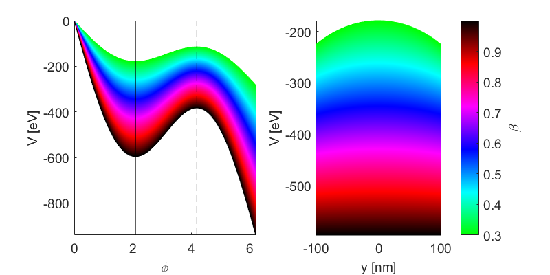
Figure 8: The potential (Eq. 36) as function of $\varphi$ and $y$ at the synchronous phase indicated by the solid vertical line. The longitudinally unstable fixed point (dashed line) flips the sign of the transverse potential. The color scale indicates the adiabatic change of the potential with $\beta$.

The full 6D Hamiltonian reads

$$H=\frac{1}{2m_{e}\gamma}\left(p_{x}^{2}+p_{y}^{2}+\Delta P_{z}^{2}\right)+V,$$ (37)

where $\Delta p_{z}/\gamma$ was replaced with $\Delta P_{z}$. The coupled equations of motion are

$$\ddot{x} =0$$ (38a)

$$\ddot{y} =-\frac{qe_{1}}{m_{e}\gamma^{2}}\sinh\left(\frac{\omega y}{\beta\gamma c}\right)\sin\left(\frac{2\pi s}{\lambda_{gz}}\right)$$ (38b)

$$\ddot{s} =\frac{qe_{1}}{m_{e}\gamma^{3}}\left(\cosh\left(\frac{\omega y}{\beta\gamma c}\right)\cos\left(\frac{2\pi s}{\lambda_{gz}}\right)-\cos\varphi_{s}\right).$$ (38c)

If the beam size is significantly smaller than the aperture ($y\ll\beta\gamma c/\omega$), the longitudinal equation decouples and becomes the ordinary differential equation of synchrotron motion. The transverse motion becomes linear in this case, however still dependent on the longitudinal motion via $\varphi$. The equation of motion,

$$\ddot{y}=\frac{-qe_{1}\omega}{m_{e}\gamma^{3}\beta c}\sin\left(\varphi\right)y,$$ (39)

is Hill’s equation, with the synchrotron angle being the focusing function. However there is a crucial difference to ordinary magnetic focusing channels. The focusing force scales as $\gamma^{-3}$ as expected for acceleration defocusing Wangler (2008), rather than with $\gamma^{-1}$ as would be expected for a magnetic quadrupole focusing channel. The solution to Eq. 39 as function of $z$ for fixed $s=\lambda_{gz}\varphi_{s}/2\pi$, i.e. when the bunch length is significantly shorter than the period length, is

$$y=y_{0}\exp\left(\sqrt{\frac{-qe_{1}\omega}{m_{e}\gamma^{3}\beta^{3}c^{3}}\sin\varphi_{s}}z\right)$$ (40)

and a synchronous particle with non-zero transverse offset is expected to grow to double transverse amplitude in

$$L_{2}=\frac{\ln 2}{\sqrt{\frac{-qe_{1}\omega}{m_{e}\gamma^{3}\beta^{3}c^{3}}\sin\varphi_{s}}}.$$ (41)

For subrelativistic particles $L_{2}$ can reach down to a few micron. However, longer interaction lengths can be achieved by focusing the beam into the DLA structure externally.

As shown in Fig. 9, the phase ranges of longitudinal and transverse focusing are disjoint. This is a consequence of Earnshaw’s theorem Earnshaw (1842) which can be directly observed in Eq. 36, i.e. V has no minima but only saddle points. Similarly as in Paul traps (see e.g. Major et al. (2005)), stable motion in both the y- and z-planes can only be achieved by rotating the saddle. For an accelerator this means alternating the synchronous phase. This so called Alternating-Phase-Focusing (APF) scheme has been developed for ion RF linacs already in the 1950’ (e.g. Fainberg (1956)) but later rejected in favor of the RFQ Wangler (2008).

Figure 9: Overview of electron acceleration and focusing properties for an x-invariant grating.

For an adiabatic Hamiltonian and if stable orbits exist, a matched locally Gaussian distribution is given by

$$f=Ce^{-H/\langle H\rangle}$$ (42)

and a locally elliptic (Hofmann-Pedersen Hofmann and Pedersen (1979)) matched distribution is given by

$$f=C\sqrt{H_{max}-H}.$$ (43)

The normalization constant $C$ is determined by integration. Note that in the case of non-periodic motion $f$ will not be integrable. Thus, we can only write a matched distribution for the longitudinal plane if $\varphi_{s}\in[\pi/2,\pi]$ and for the transverse plane if $\varphi_{s}\in[\pi,3/2\pi]$.

The Hamiltonian is not time independent, however its dependence on $\beta$ and $\gamma$ is adiabatic. Thus, if $\varphi_{s}$ is changing at most adiabatically, the distribution will deform such that the emittance increase is bounded, i.e. also the emittance remains an adiabatic invariant. First, we consider the longitudinal plane and linearized fields. For a given bunch length $\sigma_{\Delta s}$ the matched energy spread is

$$\sigma_{\Delta W}=\frac{c_{0}}{\lambda_{0}}\sqrt{-2\pi\lambda_{gz}m_{e}\gamma^{3}qe_{1}\sin\varphi_{s}}\sigma_{\Delta s}.$$ (44)

For a slow change of the potential and filling the bucket only up to a small fraction, the phase space area given by $\pi\sigma_{\Delta\varphi}\sigma_{\Delta W}$ is conserved. Moreover, using Eq. 44 a normalized bunch length and energy spread can be written as Wangler (2008)

$$\sigma_{\Delta W,n} =\frac{1}{\sqrt[4]{\beta^{3}\gamma^{3}}}\sigma_{\Delta_{W}}$$ (45a)

$$\sigma_{\Delta\varphi,n} =\sqrt[4]{\beta^{3}\gamma^{3}}\sigma_{\Delta\varphi}.$$ (45b)

Accordingly, in position and momentum coordinates, this reads

$$\sigma_{\Delta P_{z,n}} =\sqrt[4]{\frac{\beta}{\gamma}}\sigma_{\Delta P_{z}}$$ (46a)

$$\sigma_{{\Delta s},n} =\sqrt[4]{\frac{\gamma}{\beta}}\sigma_{\Delta s}.$$ (46b)

Thus the adiabatic phase damping in DLAs behaves in the same way as in RF linacs.

As a test of the code, we plot the long time evolution of the longitudinal emittance at zero transverse emittance for 3 different setups in Fig. 10.

Figure 10: Longitudinal emittance evolution for a linearly matched Gaussian beam in linearized fields, with the full fields, and with 10% excess energy spread.

First, we consider a bunch matched according to Eq. 44 in linearized fields. As expected, the symplectic code preserves the emittance in linear fields. However, the linearly matched bunch shows emittance growth in the non-linear fields. Even stronger emittance increase is to be expected, when there is a mismatch of the bunch length and the energy spread (here we chose 10% excess energy spread). The according result is obtained for the y-emittance when setting the synchronous phase into the transverse focusing regime and taking the longitudinal emittance as zero.

The effect of adiabatic damping also appears in DLAs in the transverse plane. The linearized transverse Hamiltonian reads

$$H_{\perp}=\frac{p_{y}^{2}}{2m_{e}\gamma}+\frac{qe_{1}\omega\sin\varphi_{s}}{2\beta\gamma^{2}c}y^{2}$$ (47)

and the matched momentum spread is

$$\sigma_{p_{y}}=\sqrt{\frac{m_{e}qe_{1}\omega\sin\varphi_{s}}{\beta\gamma c}}\sigma_{y}.$$ (48)

The area $\pi\sigma_{y}\sigma_{p_{y}}$ is conserved and thus we can write normalized spreads as

$$\sigma_{y,n} =\frac{1}{\sqrt[4]{\beta\gamma}}\sigma_{y}$$ (49a)

$$\sigma_{p_{y},n} =\sqrt[4]{\beta\gamma}\sigma_{p_{y}}.$$ (49b)

One observes, that for increasing beam energy the transverse beam size increases, while the momentum spread decreases. This is in accordance with the potential becoming flatter in the transverse plane, while it becomes steeper in the longitudinal plane for increasing beam energy (cf. Fig. 8).

IV.2 Tilted grating

The Hamiltonian for the tilted grating is obtained by modifying the potential (Eq. 36) as

$$V=qe_{1}\left[\frac{\lambda_{gz}}{2\pi}\cosh\left(ik_{y}y\right)\sin\left(\frac{2\pi s}{\lambda_{gz}}+\frac{2\pi x}{\lambda_{gx}}\right)-s\cos\varphi_{s}\right].$$ (50)

The coupled equations of motion are

$$\ddot{x} =-\frac{qe_{1}}{m_{e}\gamma}\frac{\lambda_{gz}}{\lambda_{gx}}\cosh\left(ik_{y}y\right)\cos\left(\frac{2\pi s}{\lambda_{gz}}+\frac{2\pi x}{\lambda_{gx}}\right)$$ (51a)

$$\ddot{y} =\frac{-ik_{y}\lambda_{gz}qe_{1}}{2\pi m_{e}\gamma}\sinh\left(ik_{y}y\right)\sin\left(\frac{2\pi s}{\lambda_{g}z}+\frac{2\pi x}{\lambda_{gx}}\right)$$ (51b)

$$\ddot{s} =\frac{qe_{1}}{m_{e}\gamma^{3}}\left[\cosh\left(ik_{y}y\right)\cos\left(\frac{2\pi s}{\lambda_{g}z}+\frac{2\pi x}{\lambda_{gx}}\right)-\cos\varphi_{s}\right].$$ (51c)

One can observe that a bunch which is not significantly shorter than the grating period is accelerated in both positive and negative $x$-direction dependent on $s$. Therefore, a coherent deflection can only be obtained for extremely short bunches. In the following we assume no net acceleration, i.e. $\varphi_{s}=\pi/2$, and replace $s=\lambda_{0}\varphi_{s}/2\pi+\Delta s$. Since tilted gratings are outlined for the generation of wiggler radiation we restrict ourselves to the ultra-relativistic case ($\beta\rightarrow 1$) here. From Eq. 17 one finds $\pm ik_{y}=k_{x}=\omega/c\tan\alpha$, which simplifies the potential to

$$V=qe_{1}\frac{\lambda_{0}}{2\pi}\cosh\left(\frac{\omega\tan\alpha}{c}y\right)\cos\left(\frac{\omega}{c}(\Delta s+x\tan\alpha)\right).$$ (52)

The equations of motion become

$$\ddot{x} =\frac{qe_{1}}{m_{e}\gamma}\tan\alpha\cosh\left(\frac{\omega\tan\alpha}{c}y\right)\sin\left(\frac{\omega}{c}(\Delta s+x\tan\alpha)\right)$$ (53a)

$$\ddot{y} =\frac{-ik_{y}\lambda_{gz}qe_{1}}{2\pi m_{e}\gamma}\sinh\left(\frac{\omega\tan\alpha}{c}y\right)\cos\left(\frac{\omega}{c}(\Delta s+x\tan\alpha)\right)$$ (53b)

$$\ddot{\Delta s} =\frac{qe_{1}}{m_{e}\gamma^{3}}\cosh\left(\frac{\omega\tan\alpha}{c}y\right)\sin\left(\frac{\omega}{c}(\Delta s+x\tan\alpha)\right).$$ (53c)

Injecting the beam with an offset $x_{0}\ll\lambda_{0}/(4\tan\alpha)$ results in a coherent oscillation around the $x$-axis with the longitudinal period

$$\lambda_{u}=\frac{2\pi c}{\sqrt{\frac{-2\pi qe_{1}}{m_{e}\gamma\lambda_{0}}}\tan\alpha}$$ (54)

for a particle with $\Delta s=y=0$. In linearized fields, the oscillation amplitude is arbitrary. However, in the nonlinear fields, additionally to the longitudinal plane, we find ’buckets’ with a distance $\lambda_{gx}$ also in the $x$-plane. These buckets split a ribbon beam which is large in x-direction into multiple beamlets, where the momentum spread acceptance is maximum at zero and vanishes at $\lambda_{gx}/2$, where integer multiples of $\lambda_{gx}$ can be added.

V Applications

We apply our approach to similar experimental parameters as for the subrelativistic experiments at FAU Erlangen Breuer and Hommelhoff (2013) and the relativistic experiments at SLAC Peralta et al. (2013); Wootton et al. (2016a). Although the structures are idealized, the results are qualitatively recovered. As a next step, we show modifications and idealizations of the beam parameters, which outline the way to a microchip accelerator.

V.1 Subrelativistic Acceleration

A subrelativistic DLA structure needs to be chirped in order to always fulfill the synchronicity condition 6 for the synchronous particle.

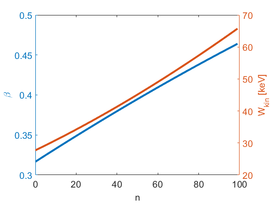
Figure 11: Acceleration ramp according to Eqs. 56 and 58.

The proper chirp for each cell and the synchronous velocity are obtained by iterating the two equations

$$\Delta z^{(n+1)}=\frac{qe_{1}\lambda_{0}^{2}\cos\varphi_{s}^{(n)}}{m_{e}c^{2}}\sqrt{1-\beta^{{(n)}^{2}}}^{3}$$ (55)

$$\beta^{(n+1)}=\beta^{(n)}+\frac{\Delta z^{(n+1)}}{\lambda_{0}}.$$ (56)

The cell length and synchronous energies are

$$\lambda_{g}^{(n)}=\lambda_{g0}+\sum\limits_{j=2}^{n}\Delta z^{(j-1)}$$ (57)

$$W_{0}^{(n)}=W_{\mathrm{init}}+qe_{1}\sum\limits_{j=2}^{n}\cos\varphi_{s}^{(j-1)}\lambda_{g}^{(j-1)}.$$ (58)

In the following simulations, we assume that the construction of the grating was made such that the cells always fulfill Eq. 57. We start with very low energy electrons $W_{\mathrm{kin}}=27.7$ keV, i.e. $\beta=0.3165$.

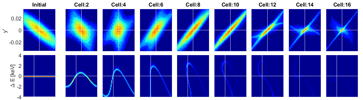
Figure 12: Longitudinal (top) and transverse (bottom) phase space for 16 cells of the chirped grating with an initially unbunched beam, focused into the structure. The axes are $100\mathrm{nm}<y<100\mathrm{nm}$ and $0<\varphi<2\pi$. The color represents the phase space density, where the initial plots are normalized to their maximum and all other plots are normalized to the respective maxima of the second column.

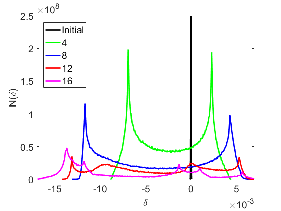
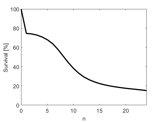
Figure 13: Energy spectra and particle survival rate for the unbunched beam.

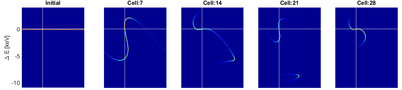
Figure 14: Longitudinal phase space evolution for zero transverse emittance. The vertical axis is $0<\varphi<2\pi$.

For $\lambda_{0}=1.96\;\mu$m the initial grating period is 620 nm. For simplicity we assume ${e_{1}=1}$ GV/m with zero phase for all cells. Aiming for a gradient of 500 MeV/m, the synchronous phase has to be 120 degree. The ramp according to these parameters is depicted in Fig. 11. Since the electron bunches in the experiments are significantly longer than the grating period, we look at initially unbunched beams with $\sigma_{E}=10$ eV.

In free space, the full Rayleigh length (cf. App. A) of the beam with assumed geometric emittance 1 nm at the aperture of $A=200$ nm is $L_{R}=A^{2}/(4\varepsilon_{y})=10~{}\mu$m, i.e. about 16 cells. This requires the optimal initial focusing angle of 20 mrad. However, as shown in Fig. 12, in the presence of strong acceleration defocusing forces, the waist appears earlier, i.e. in cell 4.

The particle loss and the energy spectrum are plotted in Fig. 13. The spectrum shows clearly that only a fraction of the particles is trapped in the bucket, the particles with $\delta\approx-13\cdot 10^{-3}$ are lost, although they do not hit the aperture. The physical loss of particles happens when they reach the aperture in y-direction ($\pm 10$ nm). The longitudinal bucket capture process is illustrated more clearly for zero transverse emittance in Fig. 14, where no transverse losses appear and a full synchrotron period is displayed.

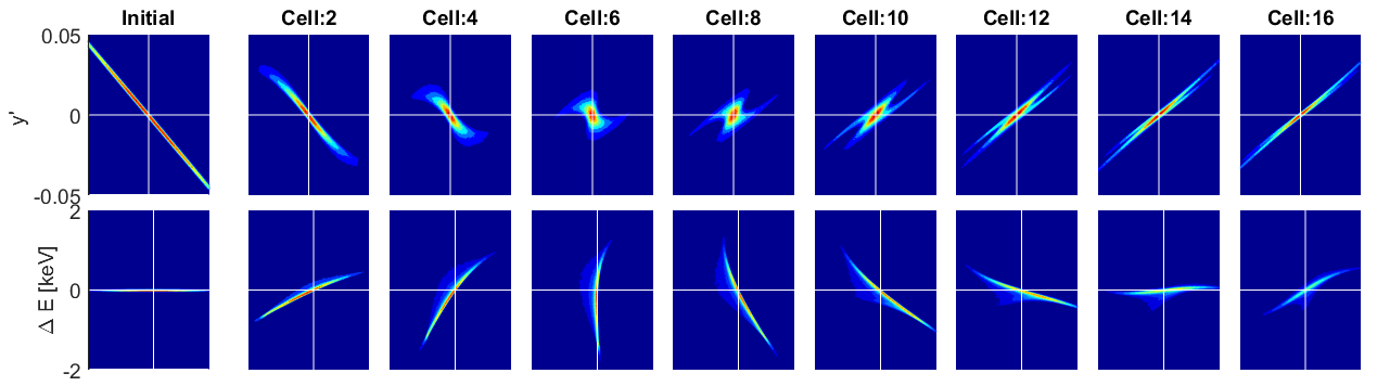
Figure 15: Longitudinal (bottom) and transverse (top) phase space for 16 cells of the chirped grating with the beam initially focused into the structure. The axes are $100\mathrm{nm}<y<100\mathrm{nm}$ and $1.5<\varphi<2.6$. Again, the color represents the phase space density, normalized to the second column.

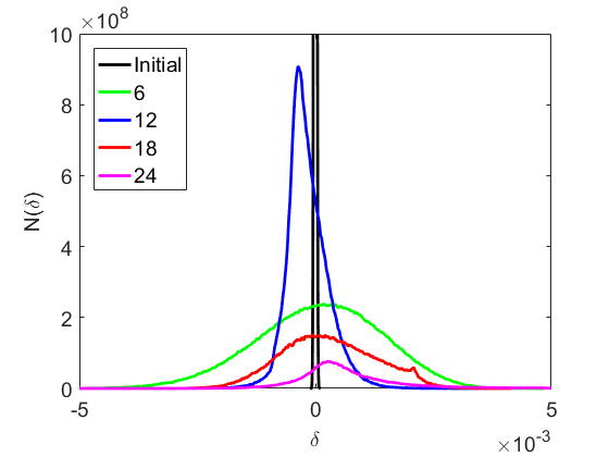
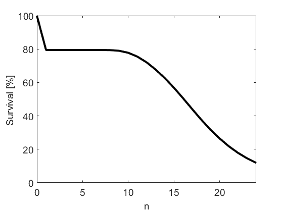
Figure 16: Energy spectra and particle survival rate for a short low energy bunch.

As next step, we take a bunched beam with $\sigma_{z}=30$ nm and a reduced transverse emittance of $\varepsilon_{y}=0.1$ nm. As shown in Fig. 15, the waist appears approximately at cell 7, when the beam is strongly focused initially with 45 mrad. Without the acceleration defocusing, the Rayleigh length would be 100 $\mu$m at an initial focusing angle of 2 mrad. The bunch has initially again an energy spread of 10 eV, which is significantly smaller than the matched energy spread. Thus a coherent quadrupole oscillation appears, which is also visible in the energy spectrum in Fig. 16.

V.2 Relativistic Acceleration

In this example we take the full aperture to be $A=800$ nm, $\lambda_{g}=\lambda_{0}=1.96\,\mu$m, $|\underline{e}_{1}|=1$ GV/m, and the number of grating cells is 100. Taking the reference particle on-crest, i.e. $\varphi_{s}=\pi$, the design ramp is linear with a slope of 1 GeV/m.

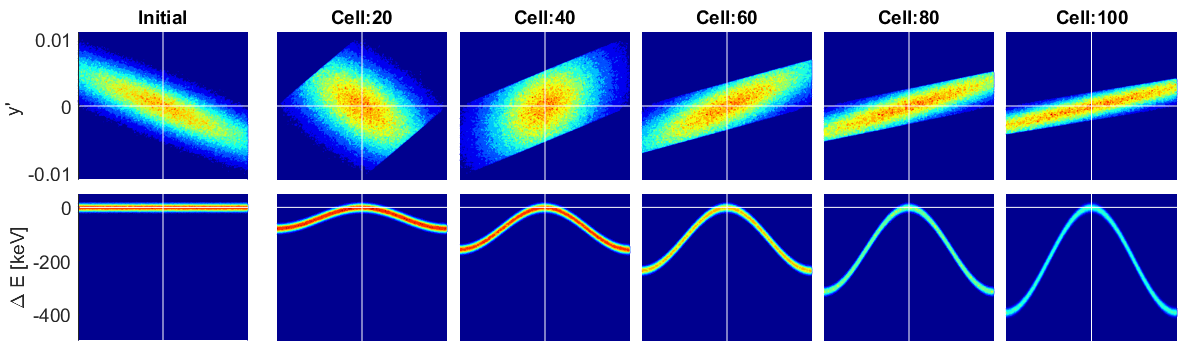
Figure 17: Evolution of the y and z phase spaces. The axes are $400\mathrm{nm}<y<400\mathrm{nm}$ and $0<\varphi<2\pi$. Again, the color represents the phase space density, normalized to the second column.

The incident electron beam has a bunch length significantly larger than the grating period and is again assumed as unbunched. The kinetic energy is 60 MeV and the spread is $\sigma_{W}=10$ keV. The spot size is taken as $\sigma_{y}=400$ nm and the geometric emittance $\varepsilon_{y}=1$ nm. The full Rayleigh range is thus $L_{R}=A^{2}/(4\varepsilon_{y})=160\;\mu$m, which is practically achieved when the beam is focused with 5 mrad into the structure. Figure 17 shows the evolution of the y and z phase spaces.

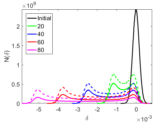
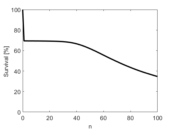
Figure 18: Energy spectra with 1 nm (solid lines) and zero (dashed lines) transverse emittance normalized to the initial number of particles $10^{6}$ (left) and particle survival rate (right).

The particle loss is monitored in Fig. 18, where the first jump is again the loss at the initial aperture. The plateau is within the Rayleigh range, however already before the end of the Rayleigh range the particles with excess momentum are being lost. Exactly at the Rayleigh range (after cell 81), the particle, that was initially the intersection of the ellipse diagonal with the aperture, is lost. The acceleration defocusing plays only a minor role for highly relativistic beams, i.e. the Rayleigh range is not significantly shortened. Figure 18 shows also the energy spectrum which becomes broader along the grating. This is due to particles being accelerated and decelerated according to their phase. Such spectra were also practically measured in Peralta et al. (2013); Wootton et al. (2016a). The dashed lines in the plot show the same spectra in the case of zero transverse emittance, where also no loss on the aperture occurs.

V.3 Dynamics in Tilted Gratings

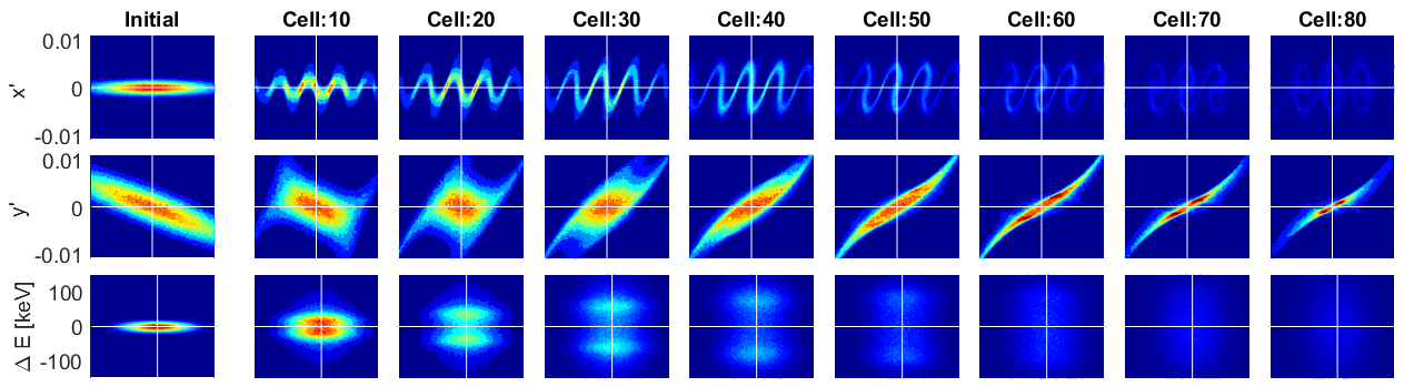
Figure 19: Horizontal, vertical, and longitudinal phase space projection for every tenth cell. The axes are $-1.5\;\mu\mathrm{m}<x<1.5\;\mu\mathrm{m}$, $-0.4\;\mu\mathrm{m}<y<0.4\;\mu\mathrm{m}$ and $1.3<\varphi<1.8$. Again, the color represents the phase space density, normalized to the second column.

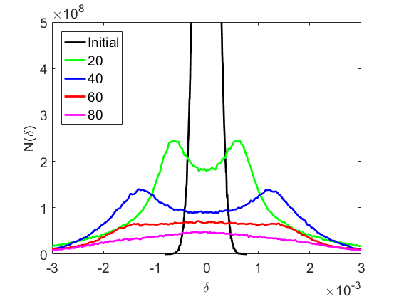
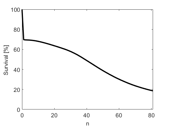
Figure 20: Evolution of the energy spectrum and particle loss.

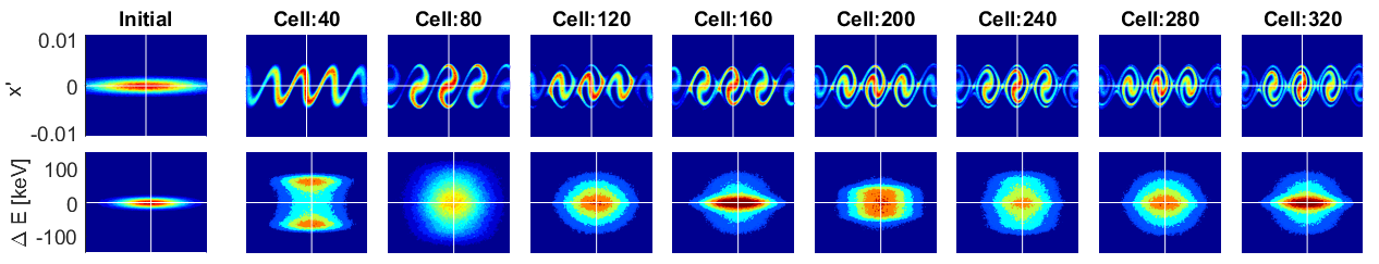
Figure 21: Horizontal and longitudinal phase space for every fortieth cell for $\varepsilon_{y}=0$. The axes are $-1.5\;\mu\mathrm{m}<x<1.5\;\mu\mathrm{m}$ and $1.3<\varphi<1.8$. Two periods of transverse oscillations are visible (cf. Eq. 54).

Finally, we address the tilted grating with the same laser parameters and a bunched electron beam with parameters $\varepsilon_{x}=\varepsilon_{y}=1$ nm, $\sigma_{x}=1\,\mu$m, $\sigma_{y}=0.4\,\mu$m, $\sigma_{z}=30$ nm, $\sigma_{W}=10$ keV and a focusing angle of 5 mrad in the y-direction. The grating tilt angle is 70 degrees and again $|\underline{e}_{1}|=1$ GV/m. Figure 19 shows the evolution of the phase space in all three planes. Evaluating Eq. 54, one finds $\lambda_{u}\approx 160\lambda_{0}$, i.e. half an oscillation period in the x-direction in the displayed 80 grating cells.

As visible in Fig. 19, the horizontal and longitudinal phase spaces are correlated. The projections of the energy spectrum can be seen in Fig. 20 together with the particle loss, which takes place at the physical aperture in y-direction at $\pm 400$ nm. Unlike the straight grating with relativistic particles, the tilted grating creates a defocusing force in the y-direction which significantly decreases the Rayleigh range. The energy spread shows a breathing mode, similar to the quadrupole modes in the synchrotron motion. However, since the synchrotron motion is practically frozen due to the high $\gamma$, this mode arises entirely due to the correlation with the x-plane. Excluding the defocusing by setting $\varepsilon_{y}=0$, two coherent oscillation periods are displayed in Fig. 21.

VI Conclusion and Outlook

The laser fields in a periodic DLA grating can be represented by spatial Fourier harmonics, where only the resonant harmonic, which fulfills the Wideroe condition, provides a first order net kick. Exploiting this property, we showed that the entire 6D beam dynamics without collective effects can be modeled by applying kicks in all spatial directions once per grating period. These kicks are not independent, but analytically connected by the Panofsky-Wenzel theorem. If the structure is not periodic, but slightly chirped (quasi-periodic), our approach is still applicable. However, fringe fields at the end of the structure are neglected.

As an example we introduced a novel Bragg-reflection based grating structure, which shows a particularly high first harmonic. The structure is discussed in Niedermayer et al. (2017) and Egenolf et al. (2017) in more detail. Here we restrict ourselves in representing the grating structures by the one resonant Fourier coefficient, i.e. one complex number for each grating cell.

We also showed that our tracking approach still works for tilted gratings that have been proposed for beam deflection or optical undulators. However, in the case of curved gratings, which have been proposed for focusing, the fields cannot be determined analytically, since the decay constant is not uniform. In order to still use our tracking algorithm, the longitudinal kicks must be provided numerically for each pair of transverse coordinates.

Additionally to our fast, symplectic tracking approach, we also derived the Hamiltonian for the single particle motion in DLA structures. This allows analytical approaches to the 6D nonlinear and coupled equations of motion in DLA structures. In the case of constant synchronous phase, the longitudinal beam dynamics is identical to the one for conventional drift tube linacs. However, for longitudinally stable buckets, the transverse fields are always defocusing. Due to the high gradients in DLA, this strong defocusing cannot be compensated by ordinary means as magnets, which is particularly critical at low electron beam energy. At relativistic energies the full Rayleigh range of an externally focused beam can be reached, however this is also only in the range of several hundred microns.

In future a focusing scheme for DLA needs to be developed. One candidate is the proposed higher order harmonic focusing Naranjo et al. (2012). In order to simulate this with our code, the additional harmonic kicks would have to be implemented. The other candidate is Alternating Phase Focusing (APF), which can be directly approached with our code. In this scheme the synchronous phase is alternated between longitudinally stable and unstable ranges, similarly as a FODO cell, but instead of x-y, rather in the y-z planes.

We plan to achieve such phase jumps by inserting drift sections as already outlined in Fig. 1. Other options are to modify the accelerating Fourier coefficient in each cell, e.g. by phase masking within the structure or by active phase control of individual parts of the laser pulse. In general, we believe that this paper gives a beam dynamics foundation on which DLA structures providing stable long distance beam transport schemes can be developed.

Appendix A Rayleigh range for light and particle beams

The Rayleigh range for a particle beam can be defined in the same way as as for a light beam. The envelope of an externally focused beam is

$$w=w_{0}\sqrt{1+\left(\frac{z}{z_{0}}\right)^{2}}.$$ (59)

Inserting into the envelope equation

$$w^{\prime\prime}=w^{-3}$$ (60)

results in $w_{0}=\sqrt{z_{0}}$. The beam size is given by $a(z)=\sqrt{\varepsilon}w(z)$ and thus the Rayleigh length is $z_{0}=a_{0}^{2}/\varepsilon$, where $a_{0}$ is the beam size at the waist. The beam size at the Rayleigh length, where it is limited by the aperture, is $a_{1}=\sqrt{2}a_{0}$. The full Rayleigh range $L_{R}=2z_{0}$ as function of the full aperture $A=2a_{1}$ is thus

$$L_{R}=\frac{A^{2}}{4\varepsilon}.$$ (61)

The same result is obtained for a light beam, where the emittance is identified with the wavelength, i.e. $\varepsilon_{\mathrm{light}}=\lambda_{0}/\pi$.

References

- Peralta et al. (2013) E. a. Peralta, K. Soong, R. J. England, E. R. Colby, Z. Wu, B. Montazeri, C. McGuinness, J. McNeur, K. J. Leedle, D. Walz, E. B. Sozer, B. Cowan, B. Schwartz, G. Travish, and R. L. Byer, Nature 503, 91 (2013).
- Wootton et al. (2016a) K. P. Wootton, Z. Wu, B. M. Cowan, A. Hanuka, I. V. Makasyuk, E. A. Peralta, K. Soong, R. L. Byer, and R. J. England, Opt. Lett. 41, 2696 (2016a).
- Breuer and Hommelhoff (2013) J. Breuer and P. Hommelhoff, Physical Review Letters 111, 134803 (2013).
- Leedle et al. (2015) K. J. Leedle, R. Fabian Pease, R. L. Byer, and J. S. Harris, Optica 2, 158 (2015).
- Shimoda (1962) K. Shimoda, Applied Optics 1, 33 (1962).
- England et al. (2014) R. J. England, R. J. Noble, K. Bane, D. H. Dowell, C.-K. Ng, J. E. Spencer, S. Tantawi, Z. Wu, R. L. Byer, E. Peralta, K. Soong, C.-M. Chang, B. Montazeri, S. J. Wolf, B. Cowan, J. Dawson, W. Gai, P. Hommelhoff, Y.-C. Huang, C. Jing, C. Mcguinness, R. B. Palmer, B. Naranjo, J. Rosenzweig, G. Travish, A. Mizrahi, L. Schachter, C. Sears, G. R. Werner, and R. B. Yoder, Reviews of Modern Physics 86, 34 (2014).
- Wootton et al. (2016b) K. P. Wootton, J. McNeur, and K. J. Leedle, Reviews of Accelerator Science and Technology 09, 105 (2016b).
- MathWorks (2016) MathWorks, “Matlab,” (2016).
- Panofsky and Wenzel (1956) W. K. H. Panofsky and W. A. Wenzel, Review of Scientific Instruments 27, 31 (1956).
- Plettner and Byer (2008a) T. Plettner and R. L. Byer, Physical Review Special Topics - Accelerators and Beams 11, 1 (2008a).
- Plettner and Byer (2008b) T. Plettner and R. L. Byer, Nuclear Instruments and Methods in Physics Research, Section A: Accelerators, Spectrometers, Detectors and Associated Equipment 593, 63 (2008b).
- Plettner et al. (2009) T. Plettner, R. Byer, C. McGuinness, and P. Hommelhoff, Physical Review Special Topics - Accelerators and Beams 12, 1 (2009).
- Fallahi et al. (2016) A. Fallahi, A. Yahaghi, and F. X. Kärtner, arXiv preprint 1612.03310 (2016).
- CST (2016) CST, “CST Studio Suite,” (2016).
- Naranjo et al. (2012) B. Naranjo, A. Valloni, S. Putterman, and J. B. Rosenzweig, Physical Review Letters 109, 1 (2012).
- Niedermayer et al. (2017) U. Niedermayer, O. Boine-Frankenheim, and T. Egenolf, Journal of Physics: Conference Series 874 (2017).
- Wangler (2008) T. P. Wangler, RF Linear Accelerators (Wiley-VCH, Weinheim, 2008).
- Earnshaw (1842) S. Earnshaw, Trans. Camb. Phil. Soc. 7, 97 (1842).
- Major et al. (2005) F. Major, V. Gheorghe, and G. Werth, Charged Particle Traps (Springer, Heidelberg, 2005).
- Fainberg (1956) I. B. Fainberg, Proc. CERN Symp. High EnergyAccel Pion Phys. (1956).
- Hofmann and Pedersen (1979) A. Hofmann and F. Pedersen, IEEE Transactions on Nuclear Science 26, 3526 (1979).
- Egenolf et al. (2017) T. Egenolf, O. Boine-Frankenheim, and U. Niedermayer, Journal of Physics: Conference Series 874 (2017).