Hyperboloidal similarity coordinates and a globally stable blowup profile for supercritical wave maps

Abstract.

We consider co-rotational wave maps from (1+3)-dimensional Minkowski space into the three-sphere. This model exhibits an explicit blowup solution and we prove the asymptotic nonlinear stability of this solution in the whole space under small perturbations of the initial data. The key ingredient is the introduction of a novel coordinate system that allows one to track the evolution past the blowup time and almost up to the Cauchy horizon of the singularity. As a consequence, we also obtain a result on continuation beyond blowup.

1. Introduction

Wave maps $U:\mathbb{R}^{1,3}\to\mathbb{S}^{3}$ from $(1+3)$-dimensional Minkowski space into the three-sphere are defined as critical points of the action functional

$$\int_{\mathbb{R}^{1,3}}\partial^{\mu}U^{a}\partial_{\mu}U^{b}g_{ab}\circ U,$$ (1.1)

where $g$ is the standard round metric on $\mathbb{S}^{3}$ and Einstein’s summation convention is in force. By choosing spherical coordinates $(t,r,\theta,\varphi)$ on Minkowski space and hyperspherical coordinates on the three-sphere, one may restrict oneself to so-called co-rotational maps which take the form $U(t,r,\theta,\varphi)=(\psi(t,r),\theta,\varphi)$. Under this symmetry reduction, the Euler-Lagrange equations associated to the action (1.1) reduce to the single scalar wave equation

$$\left(\partial_{t}^{2}-\partial_{r}^{2}-\frac{2}{r}\partial_{r}\right)\psi(t,r)+\frac{\sin(2\psi(t,r))}{r^{2}}=0$$ (1.2)

for the angle $\psi$. Note that the singularity at the center $r=0$ enforces the boundary condition $\psi(t,0)=\frac{m}{2}\pi$ for $m\in\mathbb{Z}$. To begin with, we restrict ourselves to $m=0$. By testing Eq. (1.2) with $\partial_{t}\psi(t,r)$, we obtain the conserved energy

$$\int_{0}^{\infty}\left[\tfrac{1}{2}|\partial_{t}\psi(t,r)|^{2}+\tfrac{1}{2}|\partial_{r}\psi(t,r)|^{2}+\frac{\sin^{2}(\psi(t,r))}{r^{2}}\right]r^{2}dr$$ (1.3)

and finiteness of the latter requires $\lim_{r\to\infty}\psi(t,r)=n\pi$ for $n\in\mathbb{Z}$.

Despite the existence of a positive definite energy, Eq. (1.2) develops singularities in finite time. This was first demonstrated by Shatah [47] who constructed a self-similar solution $\psi_{T}(t,r)=f_{0}(\frac{r}{T-t})$ to Eq. (1.2) by a variational argument. Here, $T>0$ is a free parameter (the blowup time). In fact, $f_{0}(\rho)=2\arctan\rho$, as was observed later [57]. The solution $\psi_{T}(t,r)$ is perfectly smooth for $t<T$ but develops a gradient blowup at the spacetime point $(t,r)=(T,0)$. In [15, 22, 9, 10] it is shown that the blowup solution $\psi_{T}(t,r)=f_{0}(\frac{r}{T-t})$ is asymptotically stable in the backward lightcone of the blowup point $(T,0)$ under small perturbations of the initial data. This result leaves open two major questions which shall be addressed in the present paper:

• How does the solution behave outside the backward lightcone?

• Is it possible to continue the solution beyond the singularity in a well-defined way?

As for the second question, we note that $\psi_{T}(t,r)$ is defined for $t<T$ only. However, $\psi_{T}$ is closely related to the principal value of the argument function $\arg$ in complex analysis. More precisely, we have $\psi_{T}(t,r)=2\arg(T-t+ir)$ and this suggests that there exists a natural continuation of $\psi_{T}$ beyond the blowup time $t=T$. Indeed, the tangent half-angle formula yields the representation

$$\arg z=2\arctan\left(\frac{\mathrm{Im}\,z}{\mathrm{Re}\,z+\sqrt{(\mathrm{Re}\,z)^{2}+(\mathrm{Im}\,z)^{2}}}\right),$$

valid if $\mathrm{Im}\,z\not=0$ or $\mathrm{Re}\,z>0$, and this leads to the more general blowup solution

$$\psi_{T}^{*}(t,r):=4\arctan\left(\frac{r}{T-t+\sqrt{(T-t)^{2}+r^{2}}}\right).$$

The skeptical reader may check by a direct computation that $\psi_{T}^{*}$ is indeed a solution to Eq. (1.2) for all $t\in\mathbb{R}$ and $r>0$. The point is that $\psi_{T}^{*}$ is smooth everywhere away from the center and thus, $\psi_{T}^{*}$ extends $\psi_{T}$ smoothly beyond the blowup time $t=T$. Furthermore,

$$\lim_{r\to 0+}\psi(t,r)=2\pi$$

if $t>T$, whereas $\psi(t,0)=0$ for $t<T$. Consequently, the blowup is accompanied by a change of the boundary condition at the center. After the blowup, the solution $\psi_{T}^{*}$ settles down to the constant function $2\pi$, i.e., for any $r>0$ we have $\lim_{t\to\infty}\psi_{T}^{*}(t,r)=2\pi$.

1.1. Statement of the main result

In view of the boundary condition $\psi(t,0)=0$ it is natural to switch to the new variable

$$\widehat{u}(t,r):=\frac{\psi(t,r)}{r}.$$

In terms of $\widehat{u}$, Eq. (1.2) reads

$$\left(\partial_{t}^{2}-\partial_{r}^{2}-\frac{4}{r}\partial_{r}\right)\widehat{u}(t,r)+\frac{\sin(2r\widehat{u}(t,r))-2r\widehat{u}(t,r)}{r^{3}}=0,$$ (1.4)

which is a radial, semilinear wave equation in 5 space dimensions. For notational purposes it is convenient to rewrite Eq. (1.4) as

$$\left(\partial_{t}^{2}-\Delta_{x}\right)u(t,x)=\frac{2|x|u(t,x)-\sin(2|x|u(t,x))}{|x|^{3}}$$ (1.5)

for $u:\mathbb{R}\times\mathbb{R}^{5}\to\mathbb{R}$ given by $u(t,x)=\widehat{u}(t,|x|)$. By the above, Eq. (1.5) has the explicit one-parameter family $\{u_{T}^{*}:T\in\mathbb{R}\}$ of blowup solutions given by

$$u_{T}^{*}(t,x):=\frac{4}{|x|}\arctan\left(\frac{|x|}{T-t+\sqrt{(T-t)^{2}+|x|^{2}}}\right).$$

We introduce the following spacetime region, depicted in Fig. 1.1.

Definition 1.1.

For $T,b\in\mathbb{R}$ we set

$$\Omega_{T,b}:=\{(t,x)\in\mathbb{R}\times\mathbb{R}^{5}:0\leq t<T+b|x|\}.$$

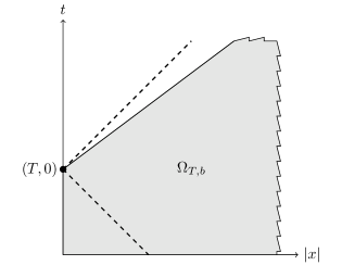
Figure 1.1. A spacetime diagram depicting the region $\Omega_{T,b}$. The dashed lines are the boundaries of the forward and backward lightcones of the point $(T,0)$. The solid line emerging from $(T,0)$ has slope $b$ and marks the upper boundary of the shaded region $\Omega_{T,b}$.

Note that $u_{T}^{*}\in C^{\infty}(\Omega_{T,b})$. Our main result establishes the stability of $u_{T}^{*}$ under small perturbations of the initial data.

Theorem 1.2.

Fix $b\in(0,1)$ and $m\in\mathbb{N}$, $m\geq 8$. Then there exist positive constants $\delta,\epsilon,M,\omega_{0}$ such that the following holds.

1. For any pair of radial functions $(f,g)\in C^{\infty}(\mathbb{R}^{5})\times C^{\infty}(\mathbb{R}^{5})$, supported in the ball $\mathbb{B}^{5}_{\epsilon}$ and satisfying

   $$\|(f,g)\|_{H^{m}(\mathbb{R}^{5})\times H^{m-1}(\mathbb{R}^{5})}\leq\tfrac{\delta}{M},$$

   there exists a $T\in[1-\delta,1+\delta]$ and a unique function $u\in C^{\infty}(\Omega_{T,b})$ that satisfies Eq. (1.5) for all $(t,x)\in\Omega_{T,b}$ and

   $$u(0,x) =u_{1}^{*}(0,x)+f(x)$$

   $$\partial_{0}u(0,x) =\partial_{0}u_{1}^{*}(0,x)+g(x)$$

   for all $x\in\mathbb{R}^{5}$.

2. The solution $u$ converges to $u_{T}^{*}$ in the sense that

   $$e^{-s}\|(u\circ\eta_{T})(s,\cdot)-(u_{T}^{*}\circ\eta_{T})(s,\cdot)\|_{H^{m-3}(\mathbb{B}^{5}_{R})} \leq\delta e^{-\omega_{0}s}$$

   $$e^{-s}\|\partial_{s}(u\circ\eta_{T})(s,\cdot)-\partial_{s}(u_{T}^{*}\circ\eta_{T})(s,\cdot)\|_{H^{m-4}(\mathbb{B}^{5}_{R})} \leq\delta e^{-\omega_{0}s}$$

   for all $s\geq 0$, where

   $$\eta_{T}(s,y) =(T+e^{-s}h(y),e^{-s}y),\qquad h(y)=\sqrt{2+|y|^{2}}-2$$

   $$R =\frac{2b+\sqrt{2(1+b^{2})}}{1-b^{2}}.$$

3. In the domain $\Omega_{T,b}\setminus\eta_{T}([s_{0},\infty)\times\mathbb{B}_{R}^{5})$, where $s_{0}=\log(-\frac{h(0)}{1+2\epsilon})$, we have $u=u_{1}^{*}$.

Remark 1.3.

It seems appropriate to comment on the comparatively high degree of regularity $m\geq 8$ in Theorem 1.2. The proof of Theorem 1.2 rests on the analysis of the evolution in a novel coordinate system which uses a hyperboloidal foliation of spacetime, see below. Therefore, it is necessary to first transport the data given at $t=0$ to the initial hyperboloid. This is done via the standard Cauchy evolution and in order to evaluate the solution on the hyperboloid, we use the Sobolev embedding which requires a sufficiently high degree of regularity. We are generous and assume $m\geq 8$.

Remark 1.4.

To avoid any possible confusion, we note that the parameter $b$ in Theorem 1.2 is fixed and only enters via $R$, i.e., it will not show up in the proofs below.

1.2. Discussion

Theorem 1.2 gives a complete description of the evolution up to the blowup time $t=T$. In particular, Theorem 1.2 shows that the solution does not develop singularities outside the backward lightcone of $(T,0)$ at some time $t<T$, a scenario which could not be ruled out by the results in [15, 22]. Furthermore, causally separated from the blowup point $(T,0)$, the evolution is controlled even beyond the blowup time and the whole region $\Omega_{T,b}$ is free of singularities. In other words, we also obtain some partial information on the evolution after the blowup. In fact, by taking $b$ close to $1$, we approach the Cauchy horizon of the singularity, that is, the boundary of the future lightcone of the point $(T,0)$, see Fig. 1.1. The solution is therefore controlled everywhere outside the future lightcone of the blowup point $(T,0)$.

The key ingredient for the proof of Theorem 1.2 is the introduction of a novel coordinate system $(s,y)$ which we call “hyperboloidal similarity coordinates” (HSC). The coordinates are defined by the function $\eta_{T}$ in Theorem 1.2, i.e.,

$$(t,x)=\eta_{T}(s,y)=(T+e^{-s}h(y),e^{-s}y),$$

and depicted in Fig. 1.2.

Figure 1.2. The hyperboloidal similarity coordinates. The hyperboloids are the lines $s=\mathrm{const}$ and the straight lines emerging radially from the blowup point $(T,0)$ correspond to $y=\mathrm{const}$. The dashed lines are the boundaries of the forward and backward lightcones of the singularity.

The coordinate system is hyperboloidal in the sense of [25, 59] but at the same time compatible with self-similarity, that is to say, the fraction $\frac{x}{T-t}=-\frac{y}{h(y)}$ is independent of the new time coordinate $s$. The hyperboloidal similarity coordinates are a generalization of the standard similarity coordinates $(\tau,\xi)=(-\log(T-t),\frac{x}{T-t})$ which are traditionally used in the study of self-similar blowup [40, 41]. By their very definition, the coordinates $(\tau,\xi)$ are restricted to $t<T$. This limitation is not present in the HSC. More precisely, the point is that the slices of constant $s$ are curved, as opposed to the constant $\tau$ slices. As a consequence, the coordinate system $(s,y)$ covers a much larger portion of spacetime than the traditional similarity coordinates $(\tau,\xi)$, see Fig. 1.2.

The bulk of the paper is concerned with the development of a nonlinear perturbation theory in the coordinates $(s,y)$ that is capable of controlling the wave maps flow near the blowup solution $u_{T}^{*}$. The approach is similar in spirit to the earlier works [15, 22], where the standard similarity coordinates $(\tau,\xi)$ are used, and based on semigroup methods, nonself-adjoint spectral theory, and ideas from infinite-dimensional dynamical systems.

1.3. Related work

The problem of finite-time blowup for wave maps attracted a lot of interest in the recent past. The bulk of the literature focuses on the two-dimensional case which is energy-critical. The existence of finite-time blowup for energy-critical wave maps into the two-sphere has first been observed numerically in the work of Bizoń-Chmaj-Tabor [5]. Rigorously, the existence of blowup solutions was proved by Krieger-Schlag-Tataru [36], Rodnianski-Sterbenz [45], and Raphaël-Rodnianski [43], see also [46, 26]. We remark that the blowup in the energy-critical case is of type II and proceeds by dynamical rescaling of a soliton, cf. [52]. In fact, there are by now powerful nonperturbative techniques for energy-critical equations which allow one to prove versions of the celebrated soliton resolution conjecture, see the work by Côte [11], Côte-Kenig-Lawrie-Schlag [12, 13], and, very recently, Jia-Kenig [33], Duyckaerts-Jia-Kenig-Merle [23], see also [31, 32]. Large-data global well-posedness and scattering is addressed in the fundamental work by Tataru-Sterbenz [50, 51] and Krieger-Schlag [38].

The present paper deals with energy-supercritical wave maps and much less is known in this case. In the equivariant setting, local well-posedness at critical regularity was settled by Shatah-Tahvildar-Zahdeh [49] and the general case is treated in the papers by Tataru [55], Tao [53, 54], Klainerman-Rodnianski [35], Shatah-Struwe [48], Nahmod-Stefanov-Uhlenbeck [42], and Krieger [37], see also [56]. For energy-supercritical equations the existence of self-similar solutions is typical and in fact, the model under investigation has plenty of them [3]. As already mentioned, the local stability of the “ground-state” self-similar solution in the backward lightcone was established in [15, 22, 9, 10], see [18, 19, 16, 21, 20] for other equations. The “ground state” actually exists in any dimension [4, 2] and its stability in the backward lightcone was recently established in [10, 7]. Furthermore, Dodson-Lawrie [14] showed that type II blowup is impossible. This, however, does not mean that every blowup is self-similar. Indeed, a novel blowup mechanism in high dimensions was discovered recently by Ghoul-Ibrahim-Nguyen [29], building on the work by Merle-Raphaël-Rodnianski [39] on the supercritical nonlinear Schrödinger equation. To avoid confusion, we remark that this type of nonself-similar blowup is also called “type II” in [29] but is different from the notion of type II blowup used by Dodson-Lawrie [14]. Furthermore, Germain [27, 28] studied self-similar wave maps, Widmayer considered the question of uniqueness of weak wave maps [58] and Chiodaroli-Krieger [8] constructed large global solutions. Finally, we remark that stable self-similar blowup also exists for wave maps with negatively curved targets [6, 17].

1.4. Notation

Most of the notation we use is standard in the field or self-explanatory. We write $\mathbb{B}_{R}^{d}(x_{0}):=\{x\in\mathbb{R}^{d}:|x-x_{0}|<R\}$ and abbreviate $\mathbb{B}_{R}^{d}:=\mathbb{B}_{R}^{d}(0)$ as well as $\mathbb{B}^{d}:=\mathbb{B}_{1}^{d}(0)$. The symbol $\mathbb{N}:=\{1,2,3,\dots\}$ denotes the natural numbers and we set $\mathbb{N}_{0}:=\{0\}\cup\mathbb{N}$. We denote by $H^{k}(\mathbb{R}^{d})$, $k\in\mathbb{N}_{0}$, the completion of the Schwartz space $\mathcal{S}(\mathbb{R}^{d})$ with respect to the Sobolev norm

$$\|f\|_{H^{k}(\mathbb{R}^{d})}^{2}:=\sum_{|\alpha|\leq k}\|\partial^{\alpha}f\|_{L^{2}(\mathbb{R}^{d})}^{2}.$$

Here, we employ the usual multi-index notation

$$\partial^{\alpha}f:=\partial_{1}^{\alpha_{1}}\partial_{2}^{\alpha_{2}}\dots\partial_{d}^{\alpha_{d}}f$$

for $\alpha=(\alpha_{1},\alpha_{2},\dots,\alpha_{d})\in\mathbb{N}_{0}^{d}$ and $|\alpha|:=\alpha_{1}+\alpha_{2}+\dots+\alpha_{d}$. The homogeneous Sobolev space $\dot{H}^{k}(\mathbb{R}^{d})$ is defined analogously but with the homogeneous Sobolev norm

$$\|f\|_{\dot{H}^{k}(\mathbb{R}^{d})}:=\sum_{|\alpha|=k}\|\partial^{\alpha}f\|_{L^{2}(\mathbb{R}^{d})}^{2}.$$

Similarly, we define $H^{k}(\mathbb{B}_{R}^{d}(x_{0}))$ as the corresponding completion of $C^{\infty}(\overline{\mathbb{B}_{R}^{d}(x_{0})})$. If $k>\frac{d}{2}$, we have $H^{k}(\mathbb{R}^{d})\hookrightarrow C(\mathbb{R}^{d})$ and we denote by $H^{k}_{\mathrm{rad}}(\mathbb{R}^{d})$ and $H^{k}_{\mathrm{rad}}(\mathbb{B}_{R}^{d})$ the subsets of $H^{k}(\mathbb{R}^{d})$ and $H^{k}(\mathbb{B}_{R}^{d})$, respectively, that consist of radial functions.

As usual, $A\lesssim B$ means that there exists a constant $C>0$ such that $A\leq CB$. Possible dependencies of the implicit constant $C$ on additional parameters follow from the context. We also write $A\simeq B$ if $A\lesssim B$ and $B\lesssim A$. In general, the letter $C$ is used to denote a constant that may change its value at each occurrence. For the sake of clarity we sometimes indicate dependencies on additional parameters by subscripts.

We follow the tradition in relativity and number the slots of functions defined on Minkowski space $\mathbb{R}^{1,d}$ starting at $0$, i.e., $\partial_{0}u(t,x)=\partial_{t}u(t,x)$. In general, Greek indices run from $0$ to $d$ whereas Latin indices run from $1$ to $d$ and Einstein’s summation convention is in force. For the signature of the Minkowski metric we use the convention that spacelike vectors have positive lengths.

For a linear operator $\mathbf{L}$ on a Banach space we denote by $\mathcal{D}(\mathbf{L})$, $\sigma(\mathbf{L})$, and $\sigma_{p}(\mathbf{L})$ its domain, spectrum, and point spectrum, respectively. Furthermore, for $\lambda\in\rho(\mathbf{L}):=\mathbb{C}\setminus\sigma(\mathbf{L})$, we set $\mathbf{R}_{\mathbf{L}}(\lambda):=(\lambda\mathbf{I}-\mathbf{L})^{-1}$. We use boldface lowercase Latin letters to denote 2-component functions, e.g. $\mathbf{f}=(f_{1},f_{2})$ and we also use the notation $[\mathbf{f}]_{j}:=f_{j}$ to extract the components.

Finally, $e_{1}:=(1,0,0,\dots,0)\in\mathbb{R}^{d}$ is the first unit vector in $\mathbb{R}^{d}$, where the dimension $d$ follows from the context.

2. Review of the standard Cauchy theory

The proof of Theorem 1.2 relies on the formulation of the problem in adapted hyperboloidal coordinates. In order to construct data on the initial hyperboloid, we employ some elementary results on the standard Cauchy theory which are reviewed in the following. For simplicity we restrict ourselves to spatial dimensions $d\geq 3$. Furthermore, we only consider wave evolution to the future starting at $t=0$. By time translation and reflection this is in fact already the most general situation.

2.1. Wave propagators

Recall that the solution of the Cauchy problem

$$\left\{\begin{array}[]{l}(\partial_{t}^{2}-\Delta_{x})u(t,x)=0,\quad(t,x)\in\mathbb{R}^{1,d}\\ u(0,\cdot)=f,\qquad\partial_{0}u(0,\cdot)=g\end{array}\right.$$ (2.1)

for $f,g\in\mathcal{S}(\mathbb{R}^{d})$, say, is given by

$$u(t,\cdot)=\cos(t|\nabla|)f+\frac{\sin(t|\nabla|)}{|\nabla|}g,$$ (2.2)

where $\phi(|\nabla|)f:=\mathcal{F}_{d}^{-1}(\phi(|\cdot|)\mathcal{F}_{d}f)$ for $\phi\in C(\mathbb{R})$ and $\mathcal{F}_{d}$ is the Fourier transform

$$\mathcal{F}_{d}f(\xi):=\int_{\mathbb{R}^{d}}e^{-i\xi x}f(x)dx.$$

The wave propagators $\cos(t|\nabla|)$ and $\frac{\sin(t|\nabla|)}{|\nabla|}$ extend by continuity to rough data, e.g. $(f,g)\in\dot{H}^{1}(\mathbb{R}^{d})\times L^{2}(\mathbb{R}^{d})$. This yields a canonical notion of strong solutions, i.e., one says that $u$ solves Eq. (2.1) if Eq. (2.2) holds. Note further that for any fixed $t\in\mathbb{R}$, the wave propagators map $\mathcal{S}(\mathbb{R}^{d})$ to itself because the symbols involved are smooth and bounded along with their derivatives.

2.2. Finite speed of propagation

The wave equation enjoys finite speed of propagation in the following sense.

Proposition 2.1.

Let $x_{0}\in\mathbb{R}^{d}$ and $d\geq 3$. Then there exists a continuous function $\gamma_{d}:[0,\infty)\to[1,\infty)$ such that

$$\|\partial_{t}^{\ell}\cos(t|\nabla|)f\|_{\dot{H}^{k}(\mathbb{B}_{T-t}^{d}(x_{0}))} \leq\|f\|_{\dot{H}^{k+\ell}(\mathbb{B}^{d}_{T}(x_{0}))}$$

$$\left\|\partial_{t}^{\ell}\frac{\sin(t|\nabla|)}{|\nabla|}f\right\|_{\dot{H}^{k}(\mathbb{B}^{d}_{T-t}(x_{0}))} \leq\|f\|_{\dot{H}^{k+\ell-1}(\mathbb{B}^{d}_{T}(x_{0}))}$$

as well as

$$\|\partial_{t}^{\ell}\cos(t|\nabla|)f\|_{L^{2}(\mathbb{B}_{T-t}^{d}(x_{0}))} \leq\gamma_{d}(T)\|f\|_{H^{1+\ell}(\mathbb{B}^{d}_{T}(x_{0}))}$$

$$\left\|\partial_{t}^{\ell}\frac{\sin(t|\nabla|)}{|\nabla|}f\right\|_{L^{2}(\mathbb{B}^{d}_{T-t}(x_{0}))} \leq\gamma_{d}(T)\|f\|_{H^{\ell}(\mathbb{B}^{d}_{T}(x_{0}))}$$

for all $f\in\mathcal{S}(\mathbb{R}^{d})$, $T>0$, $t\in[0,T)$, $k\in\mathbb{N}$, and $\ell\in\mathbb{N}_{0}$.

The bounds in homogeneous Sobolev spaces $\dot{H}^{k}$ follow directly from the energy identity. The $L^{2}$-bounds are slightly more involved and in order to prove them, we need the following result which gives us control on the $L^{2}$-norm in balls in terms of the $\dot{H}^{1}$-norm and a boundary term.

Lemma 2.2.

Let $x_{0}\in\mathbb{R}^{d}$ and $d\geq 3$. Then we have

$$\|f\|_{L^{2}(\mathbb{B}^{d}_{R}(x_{0}))}^{2}\leq R^{2}\|\nabla f\|_{L^{2}(\mathbb{B}^{d}_{R}(x_{0}))}^{2}+\tfrac{d-1}{2}R\|f\|_{L^{2}(\partial\mathbb{B}^{d}_{R}(x_{0}))}^{2}$$

for all $f\in C^{1}(\overline{\mathbb{B}^{d}_{R}(x_{0})})$ and $R>0$.

Proof.

By translation we may assume $x_{0}=0$. Introducing polar coordinates $r=|x|$ and $\omega=\frac{x}{|x|}$, we compute

$$r^{\frac{d-1}{2}}f(r\omega)=\int_{0}^{r}\partial_{s}\left[s^{\frac{d-1}{2}}f(s\omega)\right]ds=\int_{0}^{r}\left[s^{\frac{d-1}{2}}\partial_{s}f(s\omega)+\tfrac{d-1}{2}s^{\frac{d-3}{2}}f(s\omega)\right]ds$$

and Cauchy-Schwarz yields

$$r^{d-1}|f(r\omega)|^{2}\leq R\int_{0}^{R}\left|s^{\frac{d-1}{2}}\partial_{s}f(s\omega)+\tfrac{d-1}{2}s^{\frac{d-3}{2}}f(s\omega)\right|^{2}ds$$

for all $r\in[0,R]$. Expanding the square, we find

$$\tfrac{1}{R}r^{d-1}|f(r\omega)|^{2} \leq\int_{0}^{R}|\partial_{s}f(s\omega)|^{2}s^{d-1}ds+(d-1)\int_{0}^{R}\underbrace{\partial_{s}f(s\omega)f(s\omega)}_{\frac{1}{2}\partial_{s}[f(s\omega)]^{2}}s^{d-2}ds$$

$$\quad+\left(\frac{d-1}{2}\right)^{2}\int_{0}^{R}f(s\omega)^{2}s^{d-3}ds$$

$$=\int_{0}^{R}|\partial_{s}f(s\omega)|^{2}s^{d-1}ds+\tfrac{d-1}{2}R^{d-2}f(R\omega)^{2}$$

$$\quad-\frac{(d-1)(d-3)}{4}\int_{0}^{R}f(s\omega)^{2}s^{d-3}ds$$

$$\leq\int_{0}^{R}|\omega^{j}\partial_{j}f(s\omega)|^{2}s^{d-1}ds+\tfrac{d-1}{2}R^{d-2}f(R\omega)^{2}.$$

Integrating this inequality yields

$$\int_{0}^{R}\int_{\mathbb{S}^{d-1}}f(r\omega)^{2}d\sigma(\omega)r^{d-1}dr \leq R^{2}\int_{0}^{R}\int_{\mathbb{S}^{d-1}}|\nabla f(r\omega)|^{2}d\sigma(\omega)r^{d-1}dr$$

$$\quad+\tfrac{d-1}{2}R^{d}\int_{\mathbb{S}^{d-1}}f(R\omega)^{2}d\sigma(\omega)$$

$$=R^{2}\|\nabla f\|_{L^{2}(\mathbb{B}^{d}_{R})}^{2}+\tfrac{d-1}{2}R\|f\|_{L^{2}(\partial\mathbb{B}^{d}_{R})}^{2},$$

which is the claim. ∎

Proof of Proposition 2.1.

Let $u(t,\cdot)=\cos(t|\nabla|)f$. Then $u(t,\cdot),\partial_{t}u(t,\cdot)\in\mathcal{S}(\mathbb{R}^{d})$ for all $t\in\mathbb{R}$, $u\in C^{\infty}(\mathbb{R}^{1,d})$, $u(0,\cdot)=f$, $\partial_{0}u(0,\cdot)=0$, and $(\partial_{t}^{2}-\Delta_{x})u(t,x)=0$. Since $\partial^{\alpha}u(t,\cdot)$ for any multi-index $\alpha\in\mathbb{N}_{0}^{d}$ satisfies the same equation, it is sufficient to consider the case $k=1$. Furthermore, by translation invariance we may assume $x_{0}=0$. We start with the case $\ell=0$. A straightforward computation yields

$$\frac{d}{dt}\left[\int_{\mathbb{B}^{d}_{T-t}}\left(|\nabla_{x}u(t,x)|^{2}+|\partial_{t}u(t,x)|^{2}\right)dx\right]\leq 0,$$

cf. the proof of Lemma C.2, and thus,

$$\|u(t,\cdot)\|_{\dot{H}^{1}(\mathbb{B}^{d}_{T-t})}^{2}=\|\nabla u(t,\cdot)\|_{L^{2}(\mathbb{B}^{d}_{T-t})}^{2}\leq\|\nabla u(0,\cdot)\|_{L^{2}(\mathbb{B}^{d}_{T})}^{2}+\|\partial_{0}u(0,\cdot)\|_{L^{2}(\mathbb{B}^{d}_{T})}^{2}=\|f\|_{\dot{H}^{1}(\mathbb{B}^{d}_{T})}^{2}$$

since $\partial_{0}u(0,\cdot)=0$.

For the $L^{2}$-bound we appeal to Lemma 2.2 and note that the energy may be augmented by a boundary term that does not destroy the monotonicity. Indeed, we have

$$\frac{d}{dt}\left[\int_{\mathbb{B}^{d}_{T-t}}\left(|\nabla_{x}u(t,x)|^{2}+|\partial_{t}u(t,x)|^{2}\right)dx+\frac{1}{T-t}\int_{\partial\mathbb{B}_{T-t}^{d}}u(t,\omega)^{2}d\sigma(\omega)\right]\leq 0,$$

see Lemma C.2. Consequently, Lemma 2.2 implies

$$\|u(t,\cdot)\|_{L^{2}(\mathbb{B}^{d}_{T-t})}^{2} \leq(T-t)^{2}\left[\|\nabla u(t,\cdot)\|_{L^{2}(\mathbb{B}^{d}_{T-t})}^{2}+\tfrac{d-1}{2}(T-t)^{-1}\|u(t,\cdot)\|_{L^{2}(\partial\mathbb{B}^{d}_{T-t})}^{2}\right]$$

$$\leq\tfrac{d-1}{2}(T-t)^{2}\left[\|\nabla u(0,\cdot)\|_{L^{2}(\mathbb{B}^{d}_{T})}^{2}+\|\partial_{0}u(0,\cdot)\|_{L^{2}(\mathbb{B}^{d}_{T})}^{2}+T^{-1}\|u(0,\cdot)\|_{L^{2}(\partial\mathbb{B}^{d}_{T})}^{2}\right]$$

$$\leq\widetilde{\gamma}_{d}(T)\|u(0,\cdot)\|_{H^{1}(\mathbb{B}^{d}_{T})}^{2}$$

for a continuous function $\widetilde{\gamma}_{d}:[0,\infty)\to[1,\infty)$, where the last step follows from the trace theorem. For $\ell\geq 1$ we repeat the above arguments with $u$ replaced by $\partial_{0}^{\ell}u$ and use the equation to transform temporal derivatives into spatial ones. The proof for the sine propagator is identical. ∎

Remark 2.3.

By approximation, finite speed of propagation holds for rough data as well.

In view of Proposition 2.1 it is natural to extend the definition of the wave propagators to functions defined on balls only. This is most conveniently realized by means of Sobolev extensions.

Lemma 2.4.

Let $d\in\mathbb{N}$ and $x_{0}\in\mathbb{R}^{d}$. For any $r>0$ there exists a linear map $\mathcal{E}_{r,x_{0},d}:L^{2}(\mathbb{B}_{r}^{d}(x_{0}))\to L^{2}(\mathbb{R}^{d})$ such that $\mathcal{E}_{r,x_{0},d}f|_{\mathbb{B}_{r}^{d}(x_{0})}=f$ a.e. and $f\in H^{k}(\mathbb{B}_{r}^{d}(x_{0}))$ for $k\in\mathbb{N}$ implies $\mathcal{E}_{r,x_{0},d}f\in H^{k}(\mathbb{R}^{d})$. Furthermore, there exists a constant $C_{r,k,d}>0$ such that

$$\|\mathcal{E}_{r,x_{0},d}f\|_{H^{k}(\mathbb{R}^{d})}\leq C_{r,k,d}\|f\|_{H^{k}(\mathbb{B}_{r}^{d}(x_{0}))}$$

for all $k\in\mathbb{N}_{0}$, $x_{0}\in\mathbb{R}^{d}$, and $f\in H^{k}(\mathbb{B}_{r}^{d}(x_{0}))$.

Proof.

From e.g. [1] we infer the existence of an extension $\mathcal{E}_{d}:L^{2}(\mathbb{B}^{d})\to L^{2}(\mathbb{R}^{d})$ such that $\mathcal{E}_{d}f|_{\mathbb{B}^{d}}=f$ a.e. and $\|\mathcal{E}_{d}f\|_{H^{k}(\mathbb{R}^{d})}\leq C_{k,d}\|f\|_{H^{k}(\mathbb{B}^{d})}$ for all $k\in\mathbb{N}_{0}$ and all $f\in H^{k}(\mathbb{B}^{d})$. Note further that $f\in H^{d}(\mathbb{B}^{d})$ implies $\mathcal{E}_{d}f\in H^{d}(\mathbb{R}^{d})\hookrightarrow C(\mathbb{R}^{d})$ by Sobolev embedding and thus, $f$ and $\mathcal{E}_{d}f$ may be identified with continuous functions such that $\mathcal{E}_{d}f|_{\mathbb{B}^{d}}=f$. For $f\in H^{d}(\mathbb{B}_{r}^{d}(x_{0}))$ we now set $\mathcal{E}_{r,x_{0},d}f(x):=\mathcal{E}_{d}(f_{1/r}(\cdot+x_{0}/r))(\frac{x-x_{0}}{r})$, where $f_{\lambda}(x):=f(\frac{x}{\lambda})$ for any $\lambda>0$. By density, $\mathcal{E}_{r,x_{0},d}$ extends to all of $L^{2}(\mathbb{B}_{r}^{d}(x_{0}))$ and it is straightforward to verify that $\mathcal{E}_{r,x_{0},d}$ has the desired properties. ∎

Definition 2.5.

Let $T>0$, $t\in[0,T)$, and $d\in\mathbb{N}$, $d\geq 3$. Then we define

$$\cos(t|\nabla|),\frac{\sin(t|\nabla|)}{|\nabla|}:L^{2}(\mathbb{B}_{T}^{d}(x_{0}))\to L^{2}(\mathbb{B}_{T-t}^{d}(x_{0}))$$

by

$$\cos(t|\nabla|)f :=\left.\left(\cos(t|\nabla|)\mathcal{E}_{T,x_{0},d}f\right)\right|_{\mathbb{B}_{T-t}^{d}(x_{0})}$$

$$\frac{\sin(t|\nabla|)}{|\nabla|}f :=\left(\left.\frac{\sin(t|\nabla|)}{|\nabla|}\mathcal{E}_{T,x_{0},d}f\right)\right|_{\mathbb{B}_{T-t}^{d}(x_{0})},$$

where $\mathcal{E}_{T,x_{0},d}$ is a Sobolev extension as in Lemma 2.4.

Remark 2.6.

Proposition 2.1 implies that Definition 2.5 is independent of the extension chosen and that the wave propagators are bounded linear maps from $H^{k}(\mathbb{B}_{T}^{d}(x_{0}))$ to $H^{k}(\mathbb{B}_{T-t}^{d}(x_{0}))$ for all $k\in\mathbb{N}_{0}$, $T>0$, $t\in[0,T)$, and $x_{0}\in\mathbb{R}^{d}$.

2.3. Local well-posedness of semilinear wave equations

Next, we turn to the local Cauchy problem for nonlinear wave equations of the form

$$\left\{\begin{array}[]{l}\partial_{t}^{2}u(t,\cdot)-\Delta u(t,\cdot)=\mathcal{N}(u(t,\cdot))\\ u(0,\cdot)=f,\quad\partial_{0}u(0,\cdot)=g\end{array}\right.,$$ (2.3)

where $\mathcal{N}$ is some nonlinear operator. In fact, we are going to restrict ourselves to the following class of admissible nonlinearities.

Definition 2.7.

Let $k\in\mathbb{N}$ and $x_{0}\in\mathbb{R}^{d}$, $d\in\mathbb{N}$. A map $\mathcal{N}:H^{k}(\mathbb{R}^{d})\to H^{k-1}_{\mathrm{loc}}(\mathbb{R}^{d})$ is called $(k,x_{0})$-admissible iff $\mathcal{N}(0)=0$ and for any $R\geq 1$ there exists a constant $C_{R,k,x_{0},d}>0$ such that

$$\|\mathcal{N}(f)-\mathcal{N}(g)\|_{H^{k-1}(\mathbb{B}_{r}^{d}(x_{0}))}\leq C_{R,k,x_{0},d}\|f-g\|_{H^{k}(\mathbb{B}_{r}^{d}(x_{0}))}$$

for all $r\in[\frac{1}{2}R,R]$ and all $f,g\in H^{k}(\mathbb{R}^{d})$ satisfying

$$\|f\|_{H^{k}(\mathbb{B}_{R}^{d}(x_{0}))}+\|g\|_{H^{k}(\mathbb{B}_{R}^{d}(x_{0}))}\leq R.$$

Remark 2.8.

For any $r>0$, a $(k,x_{0})$-admissible nonlinearity $\mathcal{N}$ naturally restricts to a map $\mathcal{N}_{r}:H^{k}(\mathbb{B}^{d}_{r}(x_{0}))\to H^{k-1}(\mathbb{B}^{d}_{r}(x_{0}))$ by

$$\mathcal{N}_{r}(f):=\mathcal{N}(\mathcal{E}_{r,x_{0},d}f)|_{\mathbb{B}^{d}_{r}(x_{0})},$$

where $\mathcal{E}_{r,x_{0},d}$ is a Sobolev extension as in Lemma 2.4. The Lipschitz bound in Definition 2.7 ensures that $\mathcal{N}_{r}$ is independent of the extension chosen. For notational convenience we will identify $\mathcal{N}$ with $\mathcal{N}_{r}$.

Definition 2.9.

Let $k\in\mathbb{N}_{0}$, $T>0$, $x_{0}\in\mathbb{R}^{d}$, $d\in\mathbb{N}$, and $T^{\prime}\in(0,T)$. The Banach space $X^{k}_{T,x_{0}}(T^{\prime})$ consists of functions

$$u:\bigcup_{t\in[0,T^{\prime}]}\{t\}\times\mathbb{B}^{d}_{T-t}(x_{0})\to\mathbb{R}$$

such that $u(t,\cdot)\in H^{k}(\mathbb{B}^{d}_{T-t}(x_{0}))$ for each $t\in[0,T^{\prime}]$ and the map $t\mapsto\|u(t,\cdot)\|_{H^{k}(\mathbb{B}^{d}_{T-t}(x_{0}))}$ is continuous on $[0,T^{\prime}]$. Furthermore, we set

$$\|u\|_{X^{k}_{T,x_{0}}(T^{\prime})}:=\max_{t\in[0,T^{\prime}]}\|u(t,\cdot)\|_{H^{k}(\mathbb{B}^{d}_{T-t}(x_{0}))}.$$

For brevity we write $X_{T}^{k}(T^{\prime}):=X_{T,0}^{k}(T^{\prime})$.

Appealing to Duhamel’s principle, we consider the following notion of solutions.

Definition 2.10.

Let $k\in\mathbb{N}$, $T>0$, $T^{\prime}\in(0,T)$, and $x_{0}\in\mathbb{R}^{d}$, $d\geq 3$. Furthermore, assume that $\mathcal{N}$ is $(k,x_{0})$-admissible. We say that a function

$$u:\bigcup_{t\in[0,T^{\prime}]}\{t\}\times\mathbb{B}^{d}_{T-t}(x_{0})\to\mathbb{R}$$

is a strong $H^{k}$ solution of Eq. (2.3) in the truncated lightcone $\bigcup_{t\in[0,T^{\prime}]}\{t\}\times\mathbb{B}^{d}_{T-t}(x_{0})\subset\mathbb{R}^{1,d}$ iff $u\in X^{k}_{T,x_{0}}(T^{\prime})$ and

$$u(t,\cdot)=\cos(t|\nabla|)u(0,\cdot)+\frac{\sin(t|\nabla|)}{|\nabla|}\partial_{0}u(0,\cdot)+\int_{0}^{t}\frac{\sin((t-s)|\nabla|)}{|\nabla|}\mathcal{N}(u(s,\cdot))ds$$

for all $t\in[0,T^{\prime}]$.

Theorem 2.11 (Local existence in lightcones).

Let $k\in\mathbb{N}$, $M_{0},T>0$, and $x_{0}\in\mathbb{R}^{d}$, $d\geq 3$. Furthermore, assume that $\mathcal{N}$ is $(k,x_{0})$-admissible. Then there exists a $T^{\prime}\in(0,T)$ such that for all $(f,g)\in H^{k}(\mathbb{B}^{d}_{T}(x_{0}))\times H^{k-1}(\mathbb{B}_{T}^{d}(x_{0}))$ satisfying

$$\|f\|_{H^{k}(\mathbb{B}^{d}_{T}(x_{0}))}+\|g\|_{H^{k-1}(\mathbb{B}_{T}^{d}(x_{0}))}\leq M_{0},$$

the initial value problem Eq. (2.3) has a strong $H^{k}$ solution $u_{f,g}$ in the truncated lightcone $\bigcup_{t\in[0,T^{\prime}]}\{t\}\times\mathbb{B}^{d}_{T-t}(x_{0})$. Furthermore, $\partial_{0}u_{f,g}\in X^{k-1}_{T,x_{0}}(T^{\prime})$ and the solution map

$$(f,g)\mapsto(u_{f,g},\partial_{0}u_{f,g})$$

is Lipschitz as a function from (a ball in) $H^{k}(\mathbb{B}^{d}_{T}(x_{0}))\times H^{k-1}(\mathbb{B}^{d}_{T}(x_{0}))$ to $X^{k}_{T,x_{0}}(T^{\prime})\times X^{k-1}_{T,x_{0}}(T^{\prime})$.

Proof.

Without loss of generality we may assume $x_{0}=0$. We set $M:=2M_{0}\gamma$, where $\gamma:=\max_{s\in[0,\frac{T}{2}]}\gamma_{d}(T-s)$ and $\gamma_{d}$ is the continuous function from Proposition 2.1. Furthermore, for $T^{\prime}\in[0,\frac{T}{2}]$ we set

$$Y(T^{\prime}):=\{u\in X_{T}^{k}(T^{\prime}):\|u\|_{X^{k}_{T}(T^{\prime})}\leq M\}$$

and define a map $\mathcal{K}_{f,g}$ on $Y(T^{\prime})$ by

$$\mathcal{K}_{f,g}(u)(t):=\cos(t|\nabla|)f+\frac{\sin(t|\nabla|)}{|\nabla|}g+\int_{0}^{t}\frac{\sin((t-s)|\nabla|)}{|\nabla|}\mathcal{N}(u(s,\cdot))ds,\quad t\in[0,T^{\prime}].$$

Let $u\in Y(T^{\prime})$. From Proposition 2.1 and Definition 2.7 we infer the existence of a constant $\alpha>0$ such that

$$\|\mathcal{K}_{f,g}(u)(t)\|_{H^{k}(\mathbb{B}^{d}_{T-t})} \leq\gamma\|f\|_{H^{k}(\mathbb{B}^{d}_{T})}+\gamma\|g\|_{H^{k-1}(\mathbb{B}^{d}_{T})}+\gamma\int_{0}^{t}\|\mathcal{N}(u(s,\cdot))\|_{H^{k-1}(\mathbb{B}^{d}_{T-s})}ds$$

$$\leq\frac{M}{2}+\alpha\gamma\int_{0}^{t}\|u(s,\cdot)\|_{H^{k}(\mathbb{B}^{d}_{T-s})}ds$$

$$\leq\frac{M}{2}+\alpha\gamma T^{\prime}\|u\|_{X^{k}_{T}(T^{\prime})}$$

$$\leq\frac{M}{2}+\alpha\gamma T^{\prime}M$$

for all $t\in[0,T^{\prime}]$. Consequently, by choosing $T^{\prime}>0$ small enough, we obtain

$$\|\mathcal{K}_{f,g}(u)\|_{X^{k}_{T}(T^{\prime})}\leq M,$$

which means that $\mathcal{K}_{f,g}(u)\in Y(T^{\prime})$ whenever $u\in Y(T^{\prime})$. Similarly, for $u,v\in Y(T^{\prime})$, we infer

$$\|\mathcal{K}_{f,g}(u)(t)-\mathcal{K}_{f,g}(v)(t)\|_{H^{k}(\mathbb{B}^{d}_{T-t})} \leq\gamma\int_{0}^{t}\|\mathcal{N}(u(s,\cdot))-\mathcal{N}(v(s,\cdot))\|_{H^{k-1}(\mathbb{B}^{d}_{T-s})}ds$$

$$\leq\alpha\gamma\,T^{\prime}\|u-v\|_{X^{k}_{T}(T^{\prime})}$$

for all $t\in[0,T^{\prime}]$, which yields

$$\|\mathcal{K}_{f,g}(u)-\mathcal{K}_{f,g}(v)\|_{X^{k}_{T}(T^{\prime})}\leq\tfrac{1}{2}\|u-v\|_{X^{k}_{T}(T^{\prime})}$$

upon choosing $T^{\prime}>0$ sufficiently small. Thus, since $Y(T^{\prime})$ is a closed subset of the Banach space $X_{T}^{k}(T^{\prime})$, the contraction mapping principle implies the existence of a fixed point $u_{f,g}\in Y(T^{\prime})$ of $\mathcal{K}_{f,g}$. Furthermore, we have

$$\partial_{t}u_{f,g}(t,\cdot)=\partial_{t}\cos(t|\nabla|)f+\partial_{t}\frac{\sin(t|\nabla|)}{|\nabla|}g+\int_{0}^{t}\partial_{t}\frac{\sin((t-s)|\nabla|)}{|\nabla|}\mathcal{N}(u_{f,g}(s,\cdot))ds$$ (2.4)

and Proposition 2.1 yields

$$\|\partial_{t}u_{f,g}(t,\cdot)\|_{H^{k-1}(\mathbb{B}^{d}_{T-t})} \lesssim\|f\|_{H^{k}(\mathbb{B}^{d}_{T})}+\|g\|_{H^{k-1}(\mathbb{B}^{d}_{T})}+\int_{0}^{t}\|\mathcal{N}(u_{f,g}(s,\cdot))\|_{H^{k-1}(\mathbb{B}^{d}_{T-s})}ds$$

$$\lesssim M_{0}+\|u_{f,g}\|_{X^{k}_{T}(T^{\prime})}$$

for all $t\in[0,T^{\prime}]$, which shows $\partial_{0}u_{f,g}\in X^{k-1}_{T}(T^{\prime})$.

It remains to prove the Lipschitz continuity of the solution map $(f,g)\mapsto u_{f,g}$. We have

$$\|u_{f,g}(t)-u_{\widetilde{f},\widetilde{g}}(t)\|_{H^{k}(\mathbb{B}^{d}_{T-t})} =\|\mathcal{K}_{f,g}(u_{f,g})(t)-\mathcal{K}_{\widetilde{f},\widetilde{g}}(u_{\widetilde{f},\widetilde{g}})(t)\|_{H^{k}(\mathbb{B}^{d}_{T-t})}$$

$$\leq\|\mathcal{K}_{f,g}(u_{f,g})(t)-\mathcal{K}_{f,g}(u_{\widetilde{f},\widetilde{g}})(t)\|_{H^{k}(\mathbb{B}^{d}_{T-t})}$$

$$\quad+\|\mathcal{K}_{f,g}(u_{\widetilde{f},\widetilde{g}})(t)-\mathcal{K}_{\widetilde{f},\widetilde{g}}(u_{\widetilde{f},\widetilde{g}})(t)\|_{H^{k}(\mathbb{B}^{d}_{T-t})}$$

$$\leq\tfrac{1}{2}\|u_{f,g}-u_{\widetilde{f},\widetilde{g}}\|_{X^{k}_{T}(T^{\prime})}$$

$$\quad+\gamma_{d}(T)\|f-\widetilde{f}\|_{H^{k}(\mathbb{B}^{d}_{T})}+\gamma_{d}(T)\|g-\widetilde{g}\|_{H^{k-1}(\mathbb{B}^{d}_{T})}$$

for all $t\in[0,T^{\prime}]$ and thus,

$$\|u_{f,g}-u_{\widetilde{f},\widetilde{g}}\|_{X^{k}_{T}(T^{\prime})}\lesssim\|(f,g)-(\widetilde{f},\widetilde{g})\|_{H^{k}(\mathbb{B}_{T}^{d})\times H^{k-1}(\mathbb{B}^{d}_{T})}.$$

Finally, from Eq. (2.4) we infer

$$\|\partial_{t}u_{f,g}(t,\cdot)-\partial_{t}u_{\widetilde{f},\widetilde{g}}(t,\cdot)\|_{H^{k-1}(\mathbb{B}_{T-t}^{d})} \lesssim\|(f,g)-(\widetilde{f},\widetilde{g})\|_{H^{k}(\mathbb{B}_{T}^{d})\times H^{k-1}(\mathbb{B}_{T}^{d})}$$

$$\quad+\int_{0}^{t}\|\mathcal{N}(u_{f,g}(s,\cdot))-\mathcal{N}(u_{\widetilde{f},\widetilde{g}}(s,\cdot))\|_{H^{k-1}(\mathbb{B}^{d}_{T-s})}ds$$

$$\lesssim\|(f,g)-(\widetilde{f},\widetilde{g})\|_{H^{k}(\mathbb{B}_{T}^{d})\times H^{k-1}(\mathbb{B}_{T}^{d})}$$

$$\quad+\|u_{f,g}-u_{\widetilde{f},\widetilde{g}}\|_{X^{k}_{T}(T^{\prime})}$$

$$\lesssim\|(f,g)-(\widetilde{f},\widetilde{g})\|_{H^{k}(\mathbb{B}_{T}^{d})\times H^{k-1}(\mathbb{B}_{T}^{d})}$$

for all $t\in[0,T^{\prime}]$, which finishes the proof. ∎

Finite speed of propagation is valid for nonlinear equations as well. This is expressed by the following uniqueness result.

Theorem 2.12 (Uniqueness in lightcones).

Let $k\in\mathbb{N}$, $T>0$, $T^{\prime}\in[0,T)$, and $x_{0}\in\mathbb{R}^{d}$, $d\geq 3$. Furthermore, assume that $\mathcal{N}$ is $(k,x_{0})$-admissible. Suppose $u$ and $v$ are both strong $H^{k}$ solutions of Eq. (2.3) in the truncated lightcone $\bigcup_{t\in[0,T^{\prime}]}\{t\}\times\mathbb{B}^{d}_{T-t}(x_{0})$ with the same initial data, i.e., $u(0,\cdot)=v(0,\cdot)$ and $\partial_{0}u(0,\cdot)=\partial_{0}v(0,\cdot)$. Then $u=v$.

Proof.

We have

$$u(t,\cdot)-v(t,\cdot)=\int_{0}^{t}\frac{\sin((t-s)|\nabla|)}{|\nabla|}\left[\mathcal{N}(u(s,\cdot))-\mathcal{N}(v(s,\cdot))\right]ds$$

and thus,

$$\|u(t,\cdot)-v(t,\cdot)\|_{H^{k}(\mathbb{B}^{d}_{T-t})} \lesssim\int_{0}^{t}\|\mathcal{N}(u(s,\cdot))-\mathcal{N}(v(s,\cdot))\|_{H^{k-1}(\mathbb{B}_{T-s}^{d})}ds$$

$$\lesssim\int_{0}^{t}\|u(s,\cdot)-v(s,\cdot)\|_{H^{k}(\mathbb{B}_{T-s}^{d})}ds$$

for all $t\in[0,T^{\prime}]$. Consequently, Gronwall’s inequality yields $\|u(t,\cdot)-v(t,\cdot)\|_{H^{k}(\mathbb{B}_{T-t}^{d})}=0$ for all $t\in[0,T^{\prime}]$. ∎

2.4. Upgrade of regularity

Now we take a different viewpoint and assume that we already have a strong $H^{k}$ solution. We would then like to conclude that the solution is in fact smooth, provided the data are smooth. To this end, we need to strengthen the assumptions on the nonlinearity. We start with an auxiliary result which will also be useful later in a different context.

Lemma 2.13.

Let $d\in\mathbb{N}$, $x_{0}\in\mathbb{R}^{d}$, $k\in\mathbb{N}$, and $k>\frac{d}{2}$. Furthermore, let $F\in C^{\infty}(\mathbb{R}\times\mathbb{R}^{d})$, $F(0,x)=\partial_{1}F(0,x)=0$ for all $x\in\mathbb{R}^{d}$, and for $f:\mathbb{R}^{d}\to\mathbb{R}$ set

$$\mathcal{N}(f)(x):=F(f(x),x).$$

Then $\mathcal{N}$ maps $H^{k}(\mathbb{R}^{d})$ to $H^{k}_{\mathrm{loc}}(\mathbb{R}^{d})$ and for any $R\geq 1$ there exists a constant $C_{R,k,x_{0},d}>0$ such that

$$\|\mathcal{N}(f)-\mathcal{N}(g)\|_{H^{k}(\mathbb{B}_{r}^{d}(x_{0}))}\leq C_{R,k,x_{0},d}\left(\|f\|_{H^{k}(\mathbb{B}_{r}^{d}(x_{0}))}+\|g\|_{H^{k}(\mathbb{B}_{r}^{d}(x_{0}))}\right)\|f-g\|_{H^{k}(\mathbb{B}_{r}^{d}(x_{0}))}$$

for all $r\in[0,R]$ and all $f,g\in H^{k}(\mathbb{B}_{r}^{d})$ satisfying $\|f\|_{H^{k}(\mathbb{B}_{r}^{d})}+\|g\|_{H^{k}(\mathbb{B}_{r}^{d})}\leq R$. In particular, $\mathcal{N}$ is $(k,x_{0})$-admissible.

Proof.

We assume without loss of generality that $x_{0}=0$ and note that the assumption $k>\frac{d}{2}$ implies $H^{k}(\mathbb{B}_{r}^{d})\hookrightarrow C(\overline{\mathbb{B}_{r}^{d}})$ for any $r>0$. Thus, elements of $H^{k}(\mathbb{B}_{r}^{d})$ can be identified with continuous functions. Furthermore, $H^{k}(\mathbb{R}^{d})$ is a Banach algebra and thus,

$$\begin{split}\|fg\|_{H^{k}(\mathbb{B}_{r}^{d})}&=\|\mathcal{E}_{r}f\mathcal{E}_{r}g\|_{H^{k}(\mathbb{B}_{r}^{d})}\leq\|\mathcal{E}_{r}f\mathcal{E}_{r}g\|_{H^{k}(\mathbb{R}^{d})}\lesssim\|\mathcal{E}_{r}f\|_{H^{k}(\mathbb{R}^{d})}\|\mathcal{E}_{r}g\|_{H^{k}(\mathbb{R}^{d})}\\ &\lesssim\|f\|_{H^{k}(\mathbb{B}_{r}^{d})}\|g\|_{H^{k}(\mathbb{B}_{r}^{d})}\end{split}$$ (2.5)

for all $r>0$ and $f,g\in H^{k}(\mathbb{B}_{r}^{d})$, where $\mathcal{E}_{r}:=\mathcal{E}_{r,0,d}$ is an extension as in Lemma 2.4.

Now we use the fundamental theorem of calculus to obtain the identity

$$\mathcal{N}(f)(x)-\mathcal{N}(g)(x) =F(f(x),x)-F(g(x),x)=\int_{0}^{1}\tfrac{d}{ds}F\big{(}sf(x)+(1-s)g(x),x\big{)}ds$$

$$=[f(x)-g(x)]\int_{0}^{1}\partial_{1}F\big{(}sf(x)+(1-s)g(x),x\big{)}ds$$

$$=[f(x)-g(x)]\int_{0}^{1}\mathcal{N}^{\prime}\big{(}sf+(1-s)g\big{)}(x)ds$$

for all $x\in\mathbb{R}^{d}$, where $\mathcal{N}^{\prime}(f)(x):=\partial_{1}F(f(x),x)$. We claim that $\mathcal{N}^{\prime}$ maps $H^{k}(\mathbb{B}_{r}^{d})$ to itself for any $r>0$ and that for any $R\geq 1$, there exists a continuous function $\gamma_{R}:[0,\infty)\to[0,\infty)$ such that

$$\|\mathcal{N}^{\prime}(f)\|_{H^{k}(\mathbb{B}_{r}^{d})}\leq\gamma_{R}(\|\mathcal{E}_{r}f\|_{H^{k}(\mathbb{R}^{d})})\|f\|_{H^{k}(\mathbb{B}_{r}^{d})}$$ (2.6)

for all $r\in(0,R]$ and $f\in H^{k}(\mathbb{B}_{r}^{d})$. Assume for the moment that this is true. Then Eq. (2.5) and the triangle inequality yield

$$\|\mathcal{N}(f)-\mathcal{N}(g)\|_{H^{k}(\mathbb{B}^{d}_{r})} \lesssim\|f-g\|_{H^{k}(\mathbb{B}_{r}^{d})}\int_{0}^{1}\left\|\mathcal{N}^{\prime}\big{(}sf+(1-s)g\big{)}\right\|_{H^{k}(\mathbb{B}_{r}^{d})}ds.$$

Furthermore,

$$\int_{0}^{1} \left\|\mathcal{N}^{\prime}\big{(}sf+(1-s)g\big{)}\right\|_{H^{k}(\mathbb{B}_{r}^{d})}ds$$

$$\leq\int_{0}^{1}\gamma_{R}\left(\|s\mathcal{E}_{r}f+(1-s)\mathcal{E}_{r}g\|_{H^{k}(\mathbb{R}^{d})}\right)\|sf+(1-s)g\|_{H^{k}(\mathbb{B}_{r}^{d})}ds$$

$$\leq\left(\|f\|_{H^{k}(\mathbb{B}_{r}^{d})}+\|g\|_{H^{k}(\mathbb{B}_{r}^{d})}\right)\int_{0}^{1}\gamma_{R}\left(\|s\mathcal{E}_{r}f+(1-s)\mathcal{E}_{r}g\|_{H^{k}(\mathbb{R}^{d})}\right)ds$$

for all $r\in(0,R]$. This yields the stated bound and finishes the proof. Consequently, it remains to prove Eq. (2.6).

To this end, we employ a smooth cut-off $\chi_{R}:\mathbb{R}^{d}\to[0,1]$ satisfying $\chi_{R}(x)=1$ for $|x|\leq R$ and $\chi_{R}(x)=0$ for $|x|\geq 2R$. We set $F_{R}(u,x):=\chi_{R}(x)\partial_{1}F(u,x)$. Then $F_{R}\in C^{\infty}(\mathbb{R}\times\mathbb{R}^{d})$ and for any compact $K\subset\mathbb{R}$ and any multi-index $\alpha\in\mathbb{N}_{0}^{1+d}$, we have $\partial^{\alpha}F_{R}\in L^{\infty}(K\times\mathbb{R}^{d})$. Furthermore, by assumption, $F_{R}(0,x)=0$ for all $x\in\mathbb{R}^{d}$. Thus, by Moser’s inequality, see e.g. [44], Theorem 6.4.1, $x\mapsto F_{R}(f(x),x)$ belongs to $H^{k}(\mathbb{R}^{d})$ for any $f\in H^{k}(\mathbb{R}^{d})$ and there exists a continuous function $\widetilde{\gamma}_{R}:[0,\infty)\to[0,\infty)$ such that

$$\|\mathcal{N}^{\prime}(f)\|_{H^{k}(\mathbb{B}_{r}^{d})} =\|F_{R}(\mathcal{E}_{r}f(\cdot),\cdot)\|_{H^{k}(\mathbb{B}_{r}^{d})}\leq\|F_{R}(\mathcal{E}_{r}f(\cdot),\cdot)\|_{H^{k}(\mathbb{R}^{d})}$$

$$\leq\widetilde{\gamma}_{R}\left(\|\mathcal{E}_{r}f\|_{H^{k}(\mathbb{R}^{d})}\right)\|\mathcal{E}_{r}f\|_{H^{k}(\mathbb{R}^{d})}$$

$$\lesssim\widetilde{\gamma}_{R}\left(\|\mathcal{E}_{r}f\|_{H^{k}(\mathbb{R}^{d})}\right)\|f\|_{H^{k}(\mathbb{B}_{r}^{d})},$$

which proves Eq. (2.6). ∎

Theorem 2.14 (Upgrade of regularity).

Let $k\in\mathbb{N}$, $k>\frac{d}{2}$, $T>0$, $T^{\prime}\in[0,T)$, and $x_{0}\in\mathbb{R}^{d}$, $d\geq 3$. Furthermore, assume that the nonlinear operator is given by $\mathcal{N}(f)(x)=F(f(x),x)$ for a function $F\in C^{\infty}(\mathbb{R}\times\mathbb{R}^{d})$ satisfying $F(0,x)=\partial_{1}F(0,x)=0$ for all $x\in\mathbb{R}^{d}$. Suppose that $u$ is a strong $H^{k}$ solution of Eq. (2.3) in the truncated lightcone $\bigcup_{t\in[0,T^{\prime}]}\{t\}\times\mathbb{B}^{d}_{T-t}(x_{0})$. If $u(0,\cdot),\partial_{0}u(0,\cdot)\in C^{\infty}(\overline{\mathbb{B}^{d}_{T}})$ then $u\in C^{\infty}(\overline{\bigcup_{t\in[0,T^{\prime}]}\{t\}\times\mathbb{B}^{d}_{T-t}(x_{0})})$ and $u$ is a classical solution, i.e.,

$$(\partial_{t}^{2}-\Delta_{x})u(t,x)=F(u(t,x),x)$$

for all $t\in[0,T^{\prime}]$ and $x\in\overline{\mathbb{B}_{T-t}^{d}(x_{0})}$.

Proof.

Without loss of generality we assume $x_{0}=0$. By assumption, we have

$$u(t,\cdot)=\cos(t|\nabla|)u(0,\cdot)+\frac{\sin(t|\nabla|)}{|\nabla|}\partial_{0}u(0,\cdot)+\int_{0}^{t}\frac{\sin((t-s)|\nabla|)}{|\nabla|}\mathcal{N}(u(s,\cdot))ds$$ (2.7)

for all $t\in[0,T^{\prime}]$. Furthermore, Lemma 2.13 yields $\mathcal{N}(u(t,\cdot))\in H^{k}(\mathbb{B}_{T-t}^{d})$ for all $t\in[0,T^{\prime}]$ and from Eq. (2.7) we infer

$$\|u(t,\cdot)\|_{H^{k+1}(\mathbb{B}_{T-t}^{d})} \lesssim\|u(0,\cdot)\|_{H^{k+1}(\mathbb{B}_{T}^{d})}+\|\partial_{0}u(0,\cdot)\|_{H^{k}(\mathbb{B}_{T}^{d})}+\int_{0}^{t}\|\mathcal{N}(u(s,\cdot))\|_{H^{k}(\mathbb{B}_{T-s}^{d})}ds$$

$$\lesssim\int_{0}^{t}\|u(s,\cdot)\|_{H^{k}(\mathbb{B}_{T-s}^{d})}ds$$

$$\lesssim\|u\|_{X^{k}_{T}(T^{\prime})},$$

which implies $u(t,\cdot)\in H^{k+1}(\mathbb{B}_{T-t}^{d})$ for all $t\in[0,T^{\prime}]$. Inductively, we find $u(t,\cdot)\in H^{\ell}(\mathbb{B}^{d}_{T-t})$ for all $t\in[0,T^{\prime}]$ and any $\ell\in\mathbb{N}_{0}$. By Sobolev embedding we therefore obtain $u(t,\cdot)\in C^{\infty}(\overline{\mathbb{B}_{T-t}^{d}})$. The same type of argument yields $\partial_{t}u(t,\cdot)\in C^{\infty}(\overline{\mathbb{B}_{T-t}^{d}})$. Furthermore, with $\mathcal{E}_{T}:=\mathcal{E}_{T,0,d}$ the extension from Lemma 2.4, we infer

$$\partial_{t}^{2}u(t,\cdot) =\partial_{t}^{2}\cos(t|\nabla|)\mathcal{E}_{T}u(0,\cdot)+\partial_{t}^{2}\frac{\sin(t|\nabla|)}{|\nabla|}\mathcal{E}_{T}\partial_{0}u(0,\cdot)$$

$$\quad+\int_{0}^{t}\partial_{t}^{2}\frac{\sin((t-s)|\nabla|)}{|\nabla|}\mathcal{E}_{T-s}\mathcal{N}(u(s,\cdot))ds+\mathcal{E}_{T-t}\mathcal{N}(u(t,\cdot))$$

$$=\Delta u(t,\cdot)+\mathcal{E}_{T-t}\mathcal{N}(u(t,\cdot))$$

and thus, $\partial_{t}^{2}u(t,x)-\Delta_{x}u(t,x)=F(u(t,x),x)$ for all $t\in[0,T^{\prime}]$ and $x\in\overline{\mathbb{B}_{T-t}^{d}(x_{0})}$. Inductively, it follows that $u\in C^{\infty}(\overline{\bigcup_{t\in[0,T^{\prime}]}\{t\}\times\mathbb{B}^{d}_{T-t}(x_{0})})$. ∎

2.5. Application to the wave maps equation

To conclude this section, we show that the above theory applies to the wave maps equation. To this end it suffices to prove that the nonlinearity in Eq. (1.5) satisfies the hypotheses of Lemma 2.13.

Lemma 2.15.

Let $F:\mathbb{R}\times\mathbb{R}^{5}\to\mathbb{R}$ be given by

$$F(u,x):=\frac{2|x|u-\sin(2|x|u)}{|x|^{3}}.$$

Then $F(0,x)=\partial_{1}F(0,x)=0$ for all $x\in\mathbb{R}^{5}$ and $F\in C^{\infty}(\mathbb{R}\times\mathbb{R}^{5})$.

Proof.

From Taylor’s theorem with integral remainder,

$$f(t_{0}+t)=\sum_{n=0}^{N}\frac{f^{(n)}(t_{0})}{n!}t^{n}+\frac{t^{N+1}}{N!}\int_{0}^{1}f^{(N+1)}(t_{0}+st)(1-s)^{N}ds,$$

we infer

$$\sin(2|x|u)=2|x|u-4|x|^{3}u^{3}\int_{0}^{1}\cos(2s|x|u)(1-s)^{2}ds$$

and thus,

$$F(u,x)=4u^{3}\int_{0}^{1}\cos(2s|x|u)(1-s)^{2}ds.$$

Since cosine is an even function, it follows that $F\in C^{\infty}(\mathbb{R}\times\mathbb{R}^{5})$ and $F(0,x)=\partial_{1}F(0,x)=0$ for all $x\in\mathbb{R}^{5}$ is obvious. ∎

3. The wave equation in hyperboloidal similarity coordinates

In this section we study the free wave equation on $\mathbb{R}^{1,d}$ in hyperboloidal similarity coordinates. In fact, we will focus on the dimensions $d=1$ and $d=5$ and restrict ourselves to the radial case.

3.1. Coordinate systems

Throughout this paper we use three different coordinate systems on (portions of) $\mathbb{R}^{1,d}$, which we consistently denote by

$$(t,x) =(t,x^{1},\dots,x^{d})=(x^{0},x^{1},\dots,x^{d})\in\mathbb{R}^{1+d}$$

$$(\tau,\xi) =(\tau,\xi^{1},\dots,\xi^{d})=(\xi^{0},\xi^{1},\dots,\xi^{d})\in\mathbb{R}^{1+d}$$

$$(s,y) =(s,y^{1},\dots,y^{d})=(y^{0},y^{1},\dots,y^{d})\in\mathbb{R}^{1+d}.$$

Naturally, $(t,x)$ are the standard Cartesian coordinates where the Minkowski metric takes the form $\eta=\mathrm{diag}(-1,1,\dots,1)$. The standard similarity coordinates $(\tau,\xi)$ are defined by

$$(t,x)=(T-e^{-\tau},e^{-\tau}\xi),$$

where $T\in\mathbb{R}$ is a free parameter. Strictly speaking, the coordinates $(\tau,\xi)$ depend on $T$ but we suppress this in the notation. We have

$$\partial_{\tau}u(T-e^{-\tau},e^{-\tau}\xi) =e^{-\tau}\partial_{0}u(T-e^{-\tau},e^{-\tau}\xi)-e^{-\tau}\xi^{j}\partial_{j}u(T-e^{-\tau},e^{-\tau}\xi)$$

$$\partial_{\xi^{j}}u(T-e^{-\tau},e^{-\tau}\xi) =e^{-\tau}\partial_{j}u(T-e^{-\tau},e^{-\tau}\xi)$$

and as a consequence, the wave operator is given by

$$-\partial^{\mu}\partial_{\mu} u(T-e^{-\tau},e^{-\tau}\xi)$$

$$=e^{2\tau}\left[\partial_{\tau}^{2}+2\xi^{j}\partial_{\xi^{j}}\partial_{\tau}-(\delta^{jk}-\xi^{j}\xi^{k})\partial_{\xi^{j}}\partial_{\xi^{k}}+\partial_{\tau}+2\xi^{j}\partial_{\xi^{j}}\right]u(T-e^{-\tau},e^{-\tau}\xi).$$

The coordinates $(s,y)$ are defined by

$$(t,x)=(T+e^{-s}h(y),e^{-s}y),$$

where again $T\in\mathbb{R}$ is a free parameter and

$$h(y):=\sqrt{2+|y|^{2}}-2$$

is called the height function. There is a high degree of arbitrariness in our choice of $h$. The only really essential property is the fact that $\{(h(y),y)\subset\mathbb{R}^{1,1}:y\in\mathbb{R}\}$ is a Cauchy surface that is asymptotic to a forward lightcone. The particular $h$ we use is convenient because it leads to comparatively simple algebraic expressions in the following. Note also that the choice $h(y)=-1$ yields the standard similarity coordinates $(\tau,\xi)$ from above. By the chain rule, we infer

$$\partial_{s}u(T+e^{-s}h(y),e^{-s}y) =-e^{-s}h(y)\partial_{0}u(T+e^{-s}h(y),e^{-s}y)-e^{-s}y^{j}\partial_{j}u(T+e^{-s}h(y),e^{-s}y)$$

$$\partial_{y^{j}}u(T+e^{-s}h(y),e^{-s}y) =e^{-s}\partial_{j}h(y)\partial_{0}u(T+e^{-s}h(y),e^{-s}y)+e^{-s}\partial_{j}u(T+e^{-s}h(y),e^{-s}y).$$

For brevity we introduce the following notation for the partial derivatives expressed in the new coordinates.

Definition 3.1.

We define

$$(\mathcal{D}_{0}v)(s,y) :=\frac{e^{s}}{y^{k}\partial_{k}h(y)-h(y)}\left[\partial_{s}+y^{k}\partial_{y^{k}}\right]v(s,y)$$

$$(\mathcal{D}_{j}v)(s,y) :=e^{s}\partial_{y^{j}}v(s,y)-\partial_{j}h(y)(\mathcal{D}_{0}v)(s,y)$$

Then we have $\mathcal{D}_{\mu}v(s,y)=\partial_{\mu}u(T+e^{-s}h(y),e^{-s}y)$ and thus,

$$\partial^{\mu}\partial_{\mu}u(T+e^{-s}h(y),e^{-s}y)=\mathcal{D}^{\mu}\mathcal{D}_{\mu}v(s,y),$$

where $v(s,y)=u(T+e^{-s}h(y),e^{-s}y)$. Note that by construction, the differential operators $\mathcal{D}_{\mu}$ and $\mathcal{D}_{\nu}$ commute. In the case $d=1$ we have

$$\mathcal{D}_{0}v(s,y) =\frac{e^{s}}{yh^{\prime}(y)-h(y)}(\partial_{s}+y\partial_{y})v(s,y)$$

$$\mathcal{D}_{1}v(s,y) =-\frac{e^{s}}{yh^{\prime}(y)-h(y)}[h^{\prime}(y)\partial_{s}+h(y)\partial_{y}]v(s,y).$$

Finally, we note that there is a convenient direct relation between the coordinates $(\tau,\xi)$ and $(s,y)$ given by

$$(\tau,\xi)=\left(s-\log(-h(y)),-\frac{y}{h(y)}\right).$$ (3.1)

In particular, this implies the identity

$$-\mathcal{D}^{\mu}\mathcal{D}_{\mu}v(s,y)=e^{2\tau}\left[\partial_{\tau}^{2}+2\xi^{j}\partial_{\xi^{j}}\partial_{\tau}-(\delta^{jk}-\xi^{j}\xi^{k})\partial_{\xi^{j}}\partial_{\xi^{k}}+\partial_{\tau}+2\xi^{j}\partial_{\xi^{j}}\right]w(\tau,\xi),$$ (3.2)

where $v(s,y)=w(s-\log(-h(y)),-y/h(y))$.

3.2. Control of the wave evolution

Let $u\in C^{2}(\mathbb{R}^{1,1})$ satisfy the wave equation

$$\partial_{t}^{2}u(t,x)-\partial_{x}^{2}u(t,x)=0.$$

Furthermore, assume that $u(t,\cdot)$ is odd for all $t\in\mathbb{R}$. In HSC we obtain

$$\begin{split}0&=\mathcal{D}_{0}^{2}v-\mathcal{D}_{1}^{2}v=(\mathcal{D}_{0}-\mathcal{D}_{1})(\mathcal{D}_{0}+\mathcal{D}_{1})v=(\mathcal{D}_{0}+\mathcal{D}_{1})(\mathcal{D}_{0}-\mathcal{D}_{1})v\end{split}$$ (3.3)

where $v(s,y)=u(T+e^{-s}h(y),e^{-s}y)$. If we set $v_{\pm}:=\mathcal{D}_{0}v\pm\mathcal{D}_{1}v$, Eq. (3.3) implies

$$\begin{split}[1-h^{\prime}(y)]\partial_{s}v_{-}(s,y)&=-[y-h(y)]\partial_{y}v_{-}(s,y)\\ [1+h^{\prime}(y)]\partial_{s}v_{+}(s,y)&=-[y+h(y)]\partial_{y}v_{+}(s,y).\end{split}$$ (3.4)

Note that $y-h(y)$ has a unique zero at $y=-\frac{1}{2}$ and $y-h(y)<0$ for $y<-\frac{1}{2}$. Geometrically, $y=\pm\frac{1}{2}$ is the boundary of the backward lightcone with tip $(T,0)$. By testing the first equation with $v_{-}$ and integrating over $[-R,R]$, we find

$$\frac{d}{ds}\int_{-R}^{R}v_{-}(s,y)^{2}[1-h^{\prime}(y)]dy =-\int_{-R}^{R}\partial_{y}[v_{-}(s,y)^{2}][y-h(y)]dy$$

$$=-v_{-}(s,y)^{2}[y-h(y)]\Big{|}_{-R}^{R}+\int_{-R}^{R}v_{-}(s,y)^{2}[1-h^{\prime}(y)]dy$$

$$\leq\int_{-R}^{R}v_{-}(s,y)^{2}[1-h^{\prime}(y)]dy,$$ (3.5)

provided $R\geq\frac{1}{2}$. Integration with respect to $s$ and $1-h^{\prime}(y)\simeq 1$ for $y\in[-R,R]$ yield the bound

$$\|v_{-}(s,\cdot)\|_{L^{2}(\mathbb{B}_{R})}\lesssim e^{s/2}\|v_{-}(s_{0},\cdot)\|_{L^{2}(\mathbb{B}_{R})}$$

for all $s\geq s_{0}$ and any fixed $s_{0}$. Analogously, we infer

$$\|v_{+}(s,\cdot)\|_{L^{2}(\mathbb{B}_{R})}\lesssim e^{s/2}\|v_{+}(s_{0},\cdot)\|_{L^{2}(\mathbb{B}_{R})}.$$ (3.6)

Consequently, from

$$\begin{split}\partial_{s}v(s,y)&=\tfrac{1}{2}e^{-s}[y-h(y)]v_{-}(s,y)-\tfrac{1}{2}e^{-s}[y+h(y)]v_{+}(s,y)\\ \partial_{y}v(s,y)&=-\tfrac{1}{2}e^{-s}[1-h^{\prime}(y)]v_{-}(s,y)+\tfrac{1}{2}e^{-s}[1+h^{\prime}(y)]v_{+}(s,y)\end{split}$$ (3.7)

we obtain the bound

$$\|v(s,\cdot)\|_{\dot{H}^{1}(\mathbb{B}_{R})}+\|\partial_{s}v(s,\cdot)\|_{L^{2}(\mathbb{B}_{R})} \lesssim e^{-s}\left(\|v_{-}(s,\cdot)\|_{L^{2}(\mathbb{B}_{R})}+\|v_{+}(s,\cdot)\|_{L^{2}(\mathbb{B}_{R})}\right)$$

$$\lesssim e^{-s/2}\left(\|v_{-}(s_{0},\cdot)\|_{L^{2}(\mathbb{B}_{R})}+\|v_{+}(s_{0},\cdot)\|_{L^{2}(\mathbb{B}_{R})}\right)$$

$$\lesssim e^{-s/2}\left(\|v(s_{0},\cdot)\|_{\dot{H}^{1}(\mathbb{B}_{R})}+\|\partial_{0}v(s_{0},\cdot)\|_{L^{2}(\mathbb{B}_{R})}\right),$$

where we have used the fact that $yh^{\prime}(y)-h(y)\geq\frac{1}{2}$ for all $y\in\mathbb{R}$. Since $u(t,\cdot)$ is assumed to be odd, we have the boundary condition $v(s,0)=u(T+e^{-s}h(0),0)=0$ for all $s\in\mathbb{R}$ and thus,

$$v(s,y)=\int_{0}^{y}\partial_{y^{\prime}}v(s,y^{\prime})dy^{\prime}$$

which, by Cauchy-Schwarz, yields the final energy estimate

$$\|v(s,\cdot)\|_{H^{1}(\mathbb{B}_{R})}+\|\partial_{s}v(s,\cdot)\|_{L^{2}(\mathbb{B}_{R})}\lesssim e^{-s/2}\left(\|v(s_{0},\cdot)\|_{H^{1}(\mathbb{B}_{R})}+\|\partial_{0}v(s_{0},\cdot)\|_{L^{2}(\mathbb{B}_{R})}\right).$$

We generalize to higher derivatives.

Lemma 3.2.

Fix $s_{0}\in\mathbb{R}$, $R\geq\frac{1}{2}$, $T\in\mathbb{R}$, and $k\in\mathbb{N}$, $k\geq 2$. Furthermore, assume that $u\in C^{k}(\mathbb{R}^{1,1})$ satisfies

$$\partial_{t}^{2}u(t,x)-\partial_{x}^{2}u(t,x)=0$$

and suppose $u(t,\cdot)$ is odd for all $t\in\mathbb{R}$. Let $v(s,y):=u(T+e^{-s}h(y),e^{-s}y)$. Then we have the bounds

$$\|v(s,\cdot)\|_{H^{\ell}(\mathbb{B}_{R})}+\|\partial_{s}v(s,\cdot)\|_{H^{\ell-1}(\mathbb{B}_{R})}\lesssim\,e^{-s/2}\left(\|v(s_{0},\cdot)\|_{H^{\ell}(\mathbb{B}_{R})}+\|\partial_{0}v(s_{0},\cdot)\|_{H^{\ell-1}(\mathbb{B}_{R})}\right)$$

for all $s\geq s_{0}$ and all $\ell\in\mathbb{N}$ satisfying $\ell\leq k$.

Proof.

Define the differential operators

$$(L_{\pm}f)(y):=-\frac{y\pm h(y)}{1\pm h^{\prime}(y)}f^{\prime}(y),\qquad(D_{\pm}f)(y):=\frac{1}{1\pm h^{\prime}(y)}f^{\prime}(y).$$

Then Eq. (3.4) can be written as

$$\partial_{s}v_{\pm}(s,\cdot)=L_{\pm}v_{\pm}(s,\cdot).$$ (3.8)

We have the commutator relation $[D_{\pm},L_{\pm}]=-D_{\pm}$ and thus, applying $D_{\pm}^{j}$ to Eq. (3.8), for $0\leq j\leq k-1$, yields

$$\partial_{s}D_{\pm}^{j}v_{\pm}(s,\cdot)=D_{\pm}^{j}L_{\pm}v_{\pm}(s,\cdot)=L_{\pm}D_{\pm}^{j}v_{\pm}(s,\cdot)-jD_{\pm}^{j}v_{\pm}(s,\cdot).$$

Consequently, by testing with $[1\pm h^{\prime}(y)]D_{\pm}^{j}v_{\pm}(s,\cdot)$, we infer

$$\|D_{\pm}^{j}v_{\pm}(s,\cdot)\|_{L^{2}(\mathbb{B}_{R})}^{2}\lesssim e^{(1-2j)s}\|D_{\pm}^{j}v_{\pm}(s_{0},\cdot)\|_{L^{2}(\mathbb{B}_{R})}^{2}$$ (3.9)

for any $0\leq j\leq k-1$, cf. (3.6). Now we claim that, for any $\ell\in\mathbb{N}_{0}$,

$$\|f\|_{H^{\ell}(\mathbb{B}_{R})}\simeq\sum_{j=0}^{\ell}\|D_{\pm}^{j}f\|_{L^{2}(\mathbb{B}_{R})}.$$ (3.10)

Suppose for the moment that Eq. (3.10) is true. Then Eq. (3.9) implies

$$\|v_{\pm}(s,\cdot)\|_{H^{\ell-1}(\mathbb{B}_{R})} \simeq\sum_{j=0}^{\ell-1}\|D_{\pm}^{j}v_{\pm}(s,\cdot)\|_{L^{2}(\mathbb{B}_{R})}\lesssim e^{s/2}\sum_{j=0}^{\ell-1}\|D_{\pm}^{j}v_{\pm}(s_{0},\cdot)\|_{L^{2}(\mathbb{B}_{R})}$$

$$\lesssim e^{s/2}\|v_{\pm}(s_{0},\cdot)\|_{H^{\ell-1}(\mathbb{B}_{R})}$$

for any $0\leq\ell\leq k$ and the claim follows from Eq. (3.7) and the boundary condition $v(s,0)=0$.

It remains to prove Eq. (3.10). Note that $1\pm h^{\prime}(y)\gtrsim 1$ for all $y\in\mathbb{B}_{R}$. Consequently, the bound $\|D_{\pm}^{j}f\|_{L^{2}(\mathbb{B}_{R})}\lesssim\|f\|_{H^{j}(\mathbb{B}_{R})}$ is trivial. Conversely,

$$D_{\pm}^{\ell}f(y)=\sum_{j=0}^{\ell-1}a_{\pm,j}(y)f^{(j)}(y)+\frac{1}{1\pm h^{\prime}(y)}f^{(\ell)}(y)$$

for functions $a_{\pm,j}\in C^{\infty}(\mathbb{R})$ and thus,

$$\|f^{(\ell)}\|_{L^{2}(\mathbb{B}_{R})}\lesssim\|D_{\pm}^{\ell}f\|_{L^{2}(\mathbb{B}_{R})}+\sum_{j=0}^{\ell-1}\|f^{(j)}\|_{L^{2}(\mathbb{B}_{R})}\lesssim\|D_{\pm}^{\ell}f\|_{L^{2}(\mathbb{B}_{R})}+\|f\|_{H^{\ell-1}(\mathbb{B}_{R})}.$$

Consequently, the claim follows inductively. ∎

Remark 3.3.

Lemma 3.2 shows that the full range of energy bounds is available in the HSC. Even better, the evolution decays exponentially in these coordinates. This is a scaling effect.

3.3. Radial wave evolution in 5 space dimensions

Let $u\in C^{\infty}(\mathbb{R}^{1,d})$ satisfy $(\partial_{t}^{2}-\Delta)u(t,\cdot)=0$ and suppose $u(t,\cdot)$ is radial. Then there exists a function $\widehat{u}\in C^{\infty}(\mathbb{R}^{1,1})$ such that $u(t,x)=\widehat{u}(t,|x|)$. In addition, $\widehat{u}(t,\cdot)$ is even and satisfies

$$(\partial_{t}^{2}-\partial_{r}^{2}-\tfrac{d-1}{r}\partial_{r})\widehat{u}(t,r)=0.$$

It is well-known that radial wave evolution in five space dimensions can be reduced to the case $d=1$. This is a consequence of the intertwining identity

$$\partial_{r}^{2}(r^{2}\partial_{r}+3r)=(r^{2}\partial_{r}+3r)(\partial_{r}^{2}+\tfrac{4}{r}\partial_{r}).$$ (3.11)

More precisely, let $\Omega\subset\mathbb{R}^{1,1}$ be a domain and suppose $\widehat{u}\in C^{3}(\Omega)$. Then it follows directly from Eq. (3.11) that $(\partial_{t}^{2}-\partial_{r}^{2}-\frac{4}{r}\partial_{r})\widehat{u}(t,r)=0$ implies $(\partial_{t}^{2}-\partial_{r}^{2})\widetilde{u}(t,r)=0$, where $\widetilde{u}(t,r):=(r^{2}\partial_{r}+3r)\widehat{u}(t,r)$. The converse is slightly more subtle. To begin with, $(\partial_{t}^{2}-\partial_{r}^{2})\widetilde{u}(t,r)=0$ implies that $(\partial_{t}^{2}-\partial_{r}^{2}-\frac{4}{r}\partial_{r})\widehat{u}(t,r)$ belongs to the kernel of $r^{2}\partial_{r}+3r$. The equation $(r^{2}\partial_{r}+3r)U(t,r)=0$ has the general solution $U(t,r)=\frac{f(t)}{r^{3}}$ for a free function $f$. Consequently, we obtain $(\partial_{t}^{2}-\partial_{r}^{2}-\frac{4}{r}\partial_{r})\widehat{u}(t,r)=0$ but only for those $t$ where $(t,0)\in\Omega$. This appears to cause problems for the evolution in HSC, cf. Fig. 1.2.

In order to deal with this issue, we first recall that

$$\mathcal{D}_{0}\widehat{v}(s,\eta)=e^{s}h_{1}(\eta)(\partial_{s}+\eta\partial_{\eta})\widehat{v}(s,\eta),\qquad h_{1}(\eta):=\frac{1}{\eta h^{\prime}(\eta)-h(\eta)}$$

and thus,

$$\mathcal{D}_{0}^{2}\widehat{v}(s,\eta) =e^{2s}h_{1}(\eta)^{2}\left[\partial_{s}^{2}+2\eta\partial_{s}\partial_{\eta}+\eta^{2}\partial_{\eta}^{2}+\left(\eta\tfrac{h_{1}^{\prime}(\eta)}{h_{1}(\eta)}+1\right)\partial_{s}+\left(\eta^{2}\tfrac{h_{1}^{\prime}(\eta)}{h_{1}(\eta)}+2\eta\right)\partial_{\eta}\right]\widehat{v}(s,\eta).$$

Similarly,

$$\mathcal{D}_{1}\widehat{v}(s,\eta)=-e^{s}h_{1}(\eta)[h^{\prime}(\eta)\partial_{s}+h(\eta)\partial_{\eta}]\widehat{v}(s,\eta)$$

and therefore,

$$\mathcal{D}_{1}^{2}\widehat{v}(s,\eta)=e^{2s}h_{1}(\eta)^{2}\Big{[} h^{\prime}(\eta)^{2}\partial_{s}^{2}+2h^{\prime}(\eta)h(\eta)\partial_{s}\partial_{y}+h(\eta)^{2}\partial_{\eta}^{2}$$

$$+\Big{(}h^{\prime\prime}(\eta)h(\eta)+h^{\prime}(\eta)^{2}+h^{\prime}(\eta)h(\eta)\tfrac{h_{1}^{\prime}(\eta)}{h_{1}(\eta)}\Big{)}\partial_{s}$$

$$+\Big{(}\tfrac{h_{1}^{\prime}(\eta)}{h_{1}(\eta)}h(\eta)^{2}+2h^{\prime}(\eta)h(\eta)\Big{)}\partial_{\eta}\Big{]}\widehat{v}(s,\eta).$$

Consequently, the radial, $d$-dimensional wave equation in HSC,

$$\mathcal{D}_{0}^{2}\widehat{v}(s,\eta)-\mathcal{D}_{1}^{2}\widehat{v}(s,\eta)-\frac{(d-1)e^{s}}{\eta}\mathcal{D}_{1}\widehat{v}(s,\eta)=0,$$

can be written as the system

$$\partial_{s}\begin{pmatrix}\widehat{v}(s,\cdot)\\ \partial_{s}\widehat{v}(s,\cdot)\end{pmatrix}=\widehat{\mathbf{L}}_{d}\begin{pmatrix}\widehat{v}(s,\cdot)\\ \partial_{s}\widehat{v}(s,\cdot)\end{pmatrix},$$ (3.12)

with the spatial differential operator

$$\widehat{\mathbf{L}}_{d}\begin{pmatrix}\widehat{f}_{1}\\ \widehat{f}_{2}\end{pmatrix}:=\begin{pmatrix}\widehat{f}_{2}\\ c_{12}\widehat{f}_{1}^{\prime\prime}+c^{d}_{11}\widehat{f}_{1}^{\prime}+c_{21}\widehat{f}_{2}^{\prime}+c^{d}_{20}\widehat{f}_{2}\end{pmatrix}$$

and the coefficients

$$c_{12}(\eta) =\frac{h(\eta)^{2}-\eta^{2}}{1-h^{\prime}(\eta)^{2}}$$

$$c^{d}_{11}(\eta) =-\frac{1}{1-h^{\prime}(\eta)^{2}}\left[\frac{(d-1)h(\eta)}{\eta h_{1}(\eta)}+[\eta^{2}-h(\eta)^{2}]\frac{h_{1}^{\prime}(\eta)}{h_{1}(\eta)}+2[\eta-h^{\prime}(\eta)h(\eta)]\right]$$

$$c_{21}(\eta) =2\frac{h^{\prime}(\eta)h(\eta)-\eta}{1-h^{\prime}(\eta)^{2}}$$

$$c^{d}_{20}(\eta) =-\frac{1}{1-h^{\prime}(\eta)^{2}}\left[\frac{(d-1)h^{\prime}(\eta)}{\eta h_{1}(\eta)}+[\eta-h^{\prime}(\eta)h(\eta)]\frac{h_{1}^{\prime}(\eta)}{h_{1}(\eta)}-h^{\prime\prime}(\eta)h(\eta)-h^{\prime}(\eta)^{2}+1\right].$$

The equation $\widetilde{u}(t,r)=(r^{2}\partial_{r}+3r)\widehat{u}(t,r)$ in HSC reads

$$\begin{split}\widetilde{v}(s,\eta)&=e^{-2s}\eta^{2}\mathcal{D}_{1}\widehat{v}(s,\eta)+3e^{-s}\eta\widehat{v}(s,\eta)\\ &=-e^{-s}\eta^{2}h_{1}(\eta)h^{\prime}(\eta)\partial_{s}\widehat{v}(s,\eta)-e^{-s}\eta^{2}h_{1}(\eta)h(\eta)\partial_{\eta}\widehat{v}(s,\eta)+3e^{-s}\eta\widehat{v}(s,\eta)\\ &=:e^{-s}\left[a_{11}(\eta)\partial_{\eta}+a_{10}(\eta)+a_{20}(\eta)\partial_{s}\right]\widehat{v}(s,\eta).\end{split}$$ (3.13)

and differentiation with respect to $s$ yields

$$\partial_{s}\widetilde{v}(s,\eta)= e^{-s}\left[-a_{11}(\eta)\partial_{\eta}-a_{10}(\eta)+[a_{10}(\eta)-a_{20}(\eta)]\partial_{s}+a_{11}(\eta)\partial_{\eta}\partial_{s}+a_{20}(\eta)\partial_{s}^{2}\right]\widehat{v}(s,\eta).$$

If we assume for the moment that $\widehat{v}$ solves Eq. (3.12) with $d=5$, we may replace $\partial_{s}^{2}\widehat{v}(s,\eta)$ by lower-order derivatives in $s$. Explicitly, this yields

$$\begin{split}\partial_{s}\widetilde{v}(s,\eta)=e^{-s}\Big{[}&a_{20}(\eta)c_{12}(\eta)\partial_{\eta}^{2}+[a_{20}(\eta)c^{5}_{11}(\eta)-a_{11}(\eta)]\partial_{\eta}-a_{10}(\eta)\\ &+[a_{20}(\eta)c_{21}(\eta)+a_{11}(\eta)]\partial_{\eta}\partial_{s}\\ &+[a_{10}(\eta)+a_{20}(\eta)(c^{5}_{20}(\eta)-1)]\partial_{s}\Big{]}\widehat{v}(s,\eta).\end{split}$$ (3.14)

We combine Eqs. (3.13) and (3.14) into the single vector-valued equation

$$\begin{pmatrix}\widetilde{v}(s,\cdot)\\ \partial_{s}\widetilde{v}(s,\cdot)\end{pmatrix}=e^{-s}\widehat{\mathbf{D}}_{5}\begin{pmatrix}\widehat{v}(s,\cdot)\\ \partial_{s}\widehat{v}(s,\cdot)\end{pmatrix}$$

with the spatial differential operator

$$\widehat{\mathbf{D}}_{5}\begin{pmatrix}\widehat{f}_{1}\\ \widehat{f}_{2}\end{pmatrix}=\begin{pmatrix}a_{11}\widehat{f}_{1}^{\prime}+a_{10}\widehat{f}_{1}+a_{20}\widehat{f}_{2}\\ b_{12}\widehat{f}_{1}^{\prime\prime}+b_{11}\widehat{f}_{1}^{\prime}+b_{10}\widehat{f}_{1}+b_{21}\widehat{f}_{2}^{\prime}+b_{20}\widehat{f}_{2}\end{pmatrix}$$

and the coefficients

$$b_{12} =a_{20}c_{12} b_{11} =a_{20}c^{5}_{11}-a_{11} b_{10} =-a_{10}$$

$$b_{21} =a_{20}c_{21}+a_{11} b_{20} =a_{10}+a_{20}(c^{5}_{20}-1).$$

The intertwining relation Eq. (3.11) now manifests itself as

$$\widehat{\mathbf{D}}_{5}\widehat{\mathbf{L}}_{5}\widehat{\mathbf{f}}=\widehat{\mathbf{L}}_{1}\widehat{\mathbf{D}}_{5}\widehat{\mathbf{f}}+\widehat{\mathbf{D}}_{5}\widehat{\mathbf{f}},$$ (3.15)

which may be verified by a straightforward (but, admittedly, lengthy) computation.

Definition 3.4.

For $R>0$, $\eta\in[-R,R]$, and $\mathbf{f}\in C^{\infty}(\overline{\mathbb{B}_{R}^{5}})^{2}$ radial, we set $\mathbf{E}_{1}\mathbf{f}(\eta):=\mathbf{f}(\eta e_{1})$. Furthermore,

$$\mathbf{D}_{5}\mathbf{f}:=\widehat{\mathbf{D}}_{5}\mathbf{E}_{1}\mathbf{f}.$$

Definition 3.5.

Let $I\subset\mathbb{R}$ be a symmetric interval around the origin and $k\in\mathbb{N}$. Then we set

$$C^{k}_{\pm}(I) :=\{f\in C^{k}(I):f(x)=\pm f(-x)\mbox{ for all }x\in I\}$$

$$C^{\infty}_{\pm}(I) :=\{f\in C^{\infty}(I):f(x)=\pm f(-x)\mbox{ for all }x\in I\}$$

$$H^{k}_{\pm}(I) :=\{f\in H^{k}(I):f(x)=\pm f(-x)\mbox{ for all }x\in I\}$$

The following result establishes the key mapping properties of $\mathbf{D}_{5}$ which, in conjunction with Lemma 3.2, yield the desired energy bounds for $v$. The proof is rather lengthy and therefore postponed to the appendix.

Proposition 3.6.

Fix $R>0$, $k\in\mathbb{N}$, and $k\geq 2$. Then the operator $\mathbf{D}_{5}$ extends to a bijective map

$$\mathbf{D}_{5}:H^{k+1}_{\mathrm{rad}}(\mathbb{B}_{R}^{5})\times H_{\mathrm{rad}}^{k}(\mathbb{B}_{R}^{5})\to H^{k}_{-}(\mathbb{B}_{R})\times H^{k-1}_{-}(\mathbb{B}_{R})$$

and we have

$$\|\mathbf{D}_{5}\mathbf{f}\|_{H^{k}(\mathbb{B}_{R})\times H^{k-1}(\mathbb{B}_{R})}\simeq\|\mathbf{f}\|_{H^{k+1}(\mathbb{B}^{5}_{R})\times H^{k}(\mathbb{B}^{5}_{R})}$$

for all $\mathbf{f}\in H^{k+1}_{\mathrm{rad}}(\mathbb{B}_{R}^{5})\times H^{k}_{\mathrm{rad}}(\mathbb{B}_{R}^{5})$.

Proof.

See Section B. ∎

3.4. Semigroup formulation

So far we have proved a priori bounds, i.e., we have assumed that the solution already exists. Now we turn to the proof of existence. To this end, we employ the machinery of strongly continuous semigroups. As before, we start with the case $d=1$. From above we know that if $u$ satisfies $\partial_{t}^{2}u(t,x)-\partial_{x}^{2}u(t,x)=0$ and $v(s,y)=u(T+e^{-s}h(y),e^{-s}y)$, then $v_{\pm}:=\mathcal{D}_{0}v\pm\mathcal{D}_{1}v$ satisfy

$$[1\pm h^{\prime}(y)]\partial_{s}v_{\pm}(s,y)=-[y\pm h(y)]\partial_{y}v_{\pm}(s,y).$$

Equivalently,

$$\partial_{s}v_{\pm}(s,\cdot)=L_{\pm}v_{\pm}(s,\cdot)$$

with the spatial differential operator

$$L_{\pm}f(y):=-\frac{y\pm h(y)}{1\pm h^{\prime}(y)}f^{\prime}(y).$$

Proposition 3.7.

Let $R\geq\tfrac{1}{2}$ and $k\in\mathbb{N}$. Then the operator $L_{\pm}:C^{\infty}(\overline{\mathbb{B}_{R}})\subset H^{k-1}(\mathbb{B}_{R})\to H^{k-1}(\mathbb{B}_{R})$ is closable and its closure $\overline{L_{\pm}}$ generates a strongly continuous one-parameter semigroup $S_{\pm}$ on $H^{k-1}(\mathbb{B}_{R})$ with the bound

$$\|S_{\pm}(s)f\|_{H^{k-1}(\mathbb{B}_{R})}\lesssim e^{s/2}\|f\|_{H^{k-1}(\mathbb{B}_{R})}$$

for all $s\geq 0$ and $f\in H^{k-1}(\mathbb{B}_{R})$.

Proof.

We define two inner products on $L^{2}(\mathbb{B}_{R})$ by

$$(f|g)_{\pm}:=\int_{-R}^{R}f(y)\overline{g(y)}[1\pm h^{\prime}(y)]dy$$

and denote the induced norms by $\|\cdot\|_{\pm}$. A straightforward integration by parts using $R\geq\frac{1}{2}$ yields the bound

$$\mathrm{Re}\,(L_{\pm}f|f)_{\pm}\leq\tfrac{1}{2}\|f\|_{\pm}^{2}$$

for all $f\in C^{\infty}(\overline{\mathbb{B}_{R}})$, cf. Eq. (3.2). Furthermore, we set

$$D_{\pm}f(y)=\frac{1}{1\pm h^{\prime}(y)}f^{\prime}(y)$$

and define an inner product

$$(f|g)_{\pm,k-1}:=\sum_{j=0}^{k-1}(D_{\pm}^{j}f|D_{\pm}^{j}g)_{\pm}$$

with induced norm $\|\cdot\|_{\pm,k-1}$. Recall from the proof of Lemma 3.2 that $\|\cdot\|_{\pm,k-1}\simeq\|\cdot\|_{H^{k-1}(\mathbb{B}_{R})}$. We have the commutator relation $[D_{\pm},L_{\pm}]=-D_{\pm}$ and thus,

$$\mathrm{Re}\,(L_{\pm}f|f)_{\pm,k-1} =\mathrm{Re}\,\sum_{j=0}^{k-1}(D_{\pm}^{j}L_{\pm}f|D_{\pm}^{j}f)_{\pm}=\sum_{j=0}^{k-1}\left[\mathrm{Re}\,(L_{\pm}D_{\pm}^{j}f|D_{\pm}^{j}f)_{\pm}-j(D_{\pm}^{j}f|D_{\pm}^{j}f)_{\pm}\right]$$

$$\leq\tfrac{1}{2}\sum_{j=0}^{k-1}\|D_{\pm}^{j}f\|_{\pm}^{2}$$

$$=\tfrac{1}{2}\|f\|_{\pm,k-1}^{2}$$

for all $f\in C^{\infty}(\overline{\mathbb{B}_{R}})$. Thus, by the Lumer-Phillips Theorem [24] it suffices to prove that the range of $1-L_{\pm}$ is dense in $H^{k-1}(\mathbb{B}_{R})$. In other words, we have to show that for each given $F\in C^{\infty}(\overline{\mathbb{B}_{R}})$, there exists an $f\in C^{\infty}(\overline{\mathbb{B}_{R}})$ such that $(1-L_{\pm})f=F$. The equation $(1-L_{+})f=F$ reads

$$\frac{y+h(y)}{1+h^{\prime}(y)}f^{\prime}(y)+f(y)=F(y).$$

An explicit solution is given by

$$f(y) =\frac{1}{y+h(y)}\int_{1/2}^{y}[1+h^{\prime}(t)]F(t)dt$$

$$=\frac{y-\frac{1}{2}}{y+h(y)}\int_{0}^{1}[1+h^{\prime}(\tfrac{1}{2}+t(y-\tfrac{1}{2}))]F(\tfrac{1}{2}+t(y-\tfrac{1}{2}))dt.$$

Since $y=\frac{1}{2}$ is the only zero of $y+h(y)$ and $1+h^{\prime}(\frac{1}{2})\not=0$, it is evident that $f\in C^{\infty}(\overline{\mathbb{B}_{R}})$. Analogously, one proves the density of the range of $1-L_{-}$ and we are done. ∎

The next lemma shows that the closure $\overline{L_{\pm}}$ acts as a classical differential operator, provided the underlying Sobolev space contains $C^{1}(\overline{\mathbb{B}_{R}})$.

Lemma 3.8.

Let $R\geq\frac{1}{2}$, $k\in\mathbb{N}$, $k\geq 3$, and consider the closure $\overline{L_{\pm}}$ of the operator $L_{\pm}:C^{\infty}(\overline{\mathbb{B}_{R}})\subset H^{k-1}(\mathbb{B}_{R})\to H^{k-1}(\mathbb{B}_{R})$. Then $\mathcal{D}(\overline{L_{\pm}})\subset C^{k-2}(\overline{\mathbb{B}_{R}})$ and we have

$$\overline{L_{\pm}}f(y)=-\frac{y\pm h(y)}{1\pm h^{\prime}(y)}f^{\prime}(y)$$

for all $f\in\mathcal{D}(\overline{L_{\pm}})$.

Proof.

Let $f\in\mathcal{D}(\overline{L_{\pm}})$. By definition, there exists a sequence $(f_{n})_{n\in\mathbb{N}}\subset C^{\infty}(\overline{\mathbb{B}_{R}})$ such that $f_{n}\to f$ and $L_{\pm}f_{n}\to\overline{L_{\pm}}f$ in $H^{k-1}(\mathbb{B}_{R})$. By Sobolev embedding we see that $f\in C^{k-2}(\overline{\mathbb{B}_{R}})$ and

$$\left|L_{\pm}f_{n}(y)+\frac{y\pm h(y)}{1\pm h^{\prime}(y)}f^{\prime}(y)\right| \lesssim\|f_{n}^{\prime}-f^{\prime}\|_{L^{\infty}(\mathbb{B}_{R})}\lesssim\|f_{n}-f\|_{H^{k-1}(\mathbb{B}_{R})}\to 0$$

as $n\to\infty$. ∎

As a corollary, we obtain classical solutions for the half-wave equations.

Corollary 3.9.

Let $R\geq\frac{1}{2}$, $k\in\mathbb{N}$, and $k\geq 3$. Furthermore, let $f_{\pm}\in C^{\infty}(\overline{\mathbb{B}_{R}})$ and set

$$v_{\pm}(s,y):=S_{\pm}(s)f_{\pm}(y),$$

where $S_{\pm}$ is the semigroup on $H^{k-1}(\mathbb{B}_{R})$ from Proposition 3.7. Then $v_{\pm}\in C^{1}([0,\infty)\times\overline{\mathbb{B}_{R}})$ and

$$(\mathcal{D}_{0}\mp\mathcal{D}_{1})v_{\pm}(s,y)=0.$$

Proof.

Since $f_{\pm}\in C^{\infty}(\overline{\mathbb{B}_{R}})\subset\mathcal{D}(\overline{L_{\pm}})$, semigroup theory implies $\partial_{s}v_{\pm}(s,\cdot)=\overline{L_{\pm}}v_{\pm}(s,\cdot)$. Consequently, Lemma 3.8 finishes the proof. ∎

Now we can easily construct a semigroup that produces a solution to the one-dimensional wave equation in HSC.

Definition 3.10.

Let $R\geq\frac{1}{2}$, $k\in\mathbb{N}$, and $k\geq 3$. For $(f_{1},f_{2})\in H^{k}(\mathbb{B}_{R})\times H^{k-1}(\mathbb{B}_{R})$ and $(f_{-},f_{+})\in H^{k-1}(\mathbb{B}_{R})\times H^{k-1}(\mathbb{B}_{R})$ we set

$$\mathbf{A}\left(\begin{array}[]{c}f_{1}\\ f_{2}\end{array}\right)(y):=\frac{1}{yh^{\prime}(y)-h(y)}\left(\begin{array}[]{c}(y+h(y))f_{1}^{\prime}(y)+(1+h^{\prime}(y))f_{2}(y)\\ (y-h(y))f_{1}^{\prime}(y)+(1-h^{\prime}(y))f_{2}(y)\end{array}\right)$$

and

$$\mathbf{B}\left(\begin{array}[]{c}f_{-}\\ f_{+}\end{array}\right)(y):=\frac{1}{2}\left(\begin{array}[]{c}-\int_{0}^{y}(1-h^{\prime}(t))f_{-}(t)dt+\int_{0}^{y}(1+h^{\prime}(t))f_{+}(t)dt\\ (y-h(y))f_{-}(y)-(y+h(y))f_{+}(y)\end{array}\right).$$

Furthermore, for $s\geq 0$, we define $\mathbf{S}_{1}(s):H^{k}(\mathbb{B}_{R})\times H^{k-1}(\mathbb{B}_{R})\to H^{k}(\mathbb{B}_{R})\times H^{k-1}(\mathbb{B}_{R})$ by

$$\mathbf{S}_{1}(s):=e^{-s}\mathbf{B}\left(\begin{array}[]{cc}S_{-}(s)&0\\ 0&S_{+}(s)\end{array}\right)\mathbf{A},$$

where $S_{\pm}$ are the semigroups on $H^{k-1}(\mathbb{B}_{R})$ constructed in Proposition 3.7.

As the following result shows, $\mathbf{S}_{1}$ is the solution operator for the one-dimensional wave equation in HSC with a Dirichlet condition at the center.

Proposition 3.11.

Let $\mathbf{f}\in C_{-}^{\infty}(\overline{\mathbb{B}_{R}})^{2}$ and set $v(s,y):=[\mathbf{S}_{1}(s)\mathbf{f}]_{1}(y)$. Then $v\in C^{2}([0,\infty)\times\overline{\mathbb{B}_{R}})$, $v(s,\cdot)$ is odd for all $s\geq 0$, and we have $\partial_{s}v(s,y)=[\mathbf{S}_{1}(s)\mathbf{f}]_{2}(y)$ as well as

$$\mathcal{D}_{0}^{2}v(s,y)-\mathcal{D}_{1}^{2}v(s,y)=0$$

for all $(s,y)\in[0,\infty)\times\overline{\mathbb{B}_{R}}$. Furthermore, the family $\{\mathbf{S}_{1}(s):s\geq 0\}$ forms a strongly continuous semigroup of bounded operators on $H_{-}^{k}(\mathbb{B}_{R})\times H_{-}^{k-1}(\mathbb{B}_{R})$ with generator

$$\mathbf{L}_{1}=\mathbf{B}\left(\begin{array}[]{cc}\overline{L_{-}}&0\\ 0&\overline{L_{+}}\end{array}\right)\mathbf{A}-\mathbf{I}.$$

Proof.

We define $v_{\pm}$ by

$$\begin{pmatrix}v_{-}(s,\cdot)\\ v_{+}(s,\cdot)\end{pmatrix}:=\begin{pmatrix}S_{-}(s)&0\\ 0&S_{+}(s)\end{pmatrix}\mathbf{A}\mathbf{f}.$$

From Corollary 3.9 we have $v_{\pm}\in C^{1}([0,\infty)\times\overline{\mathbb{B}_{R}})$ and $(\mathcal{D}_{0}\mp\mathcal{D}_{1})v_{\pm}=0$. Furthermore,

$$v_{-}(0,-y) =\frac{1}{-yh^{\prime}(-y)-h(-y)}\left[(-y+h(-y))f_{1}^{\prime}(-y)+(1+h^{\prime}(-y))f_{2}(-y)\right]$$

$$=\frac{1}{yh^{\prime}(y)-h(y)}\left[(-y+h(y))f_{1}^{\prime}(y)-(1-h^{\prime}(y))f_{2}(y)\right]$$

$$=-v_{+}(0,y).$$

Since $v_{-}(s,-y)$ satisfies the same equation as $v_{+}(s,y)$, it follows from the a priori bound Eq. (3.6) that

$$\|v_{+}(s,\cdot)+v_{-}(s,-(\cdot))\|_{L^{2}(\mathbb{B}_{R})}\lesssim e^{s/2}\|v_{+}(0,\cdot)+v_{-}(0,-(\cdot))\|_{L^{2}(\mathbb{B}_{R})}=0$$

and thus, $v_{-}(s,-y)=-v_{+}(s,y)$ for all $(s,y)\in[0,\infty)\times\overline{\mathbb{B}_{R}}$. Consequently, the function $y\mapsto-(1-h^{\prime}(y))v_{-}(s,y)+(1+h^{\prime}(y))v_{+}(s,y)$ is even, whereas $y\mapsto(y-h(y))v_{-}(s,y)-(y+h(y))v_{+}(s,y)$ is odd. This shows that $\mathbf{S}_{1}(s)$ maps odd functions to odd functions. The first statement now follows from Eq. (3.7) (or a straightforward computation). To prove the semigroup property, we first note that $\mathbf{A}\mathbf{B}=\mathbf{I}$ and thus,

$$\mathbf{S}_{1}(s+t) =e^{-s-t}\mathbf{B}\left(\begin{array}[]{cc}S_{-}(s+t)&0\\ 0&S_{+}(s+t)\end{array}\right)\mathbf{A}$$

$$=e^{-s-t}\mathbf{B}\left(\begin{array}[]{cc}S_{-}(s)&0\\ 0&S_{+}(s)\end{array}\right)\mathbf{A}\mathbf{B}\left(\begin{array}[]{cc}S_{-}(t)&0\\ 0&S_{+}(t)\end{array}\right)\mathbf{A}$$

$$=\mathbf{S}_{1}(s)\mathbf{S}_{1}(t)$$

for all $s,t\geq 0$. Furthermore, it is obvious that $s\mapsto\mathbf{S}_{1}(s)$ is strongly continuous. Finally, $\mathbf{S}_{1}(0)\mathbf{f}=\mathbf{B}\mathbf{A}\mathbf{f}=\mathbf{f}$ since $\mathbf{f}$ is odd. The statement about the generator is obvious. ∎

By conjugating with $\mathbf{D}_{5}$, we obtain the solution operator for the 5-dimensional wave equation. This leads to the main result of this section.

Definition 3.12.

For $s\geq 0$ we define $\mathbf{S}_{5}(s):H^{k+1}_{\mathrm{rad}}(\mathbb{B}_{R}^{5})\times H^{k}_{\mathrm{rad}}(\mathbb{B}_{R}^{5})\to H^{k+1}_{\mathrm{rad}}(\mathbb{B}_{R}^{5})\times H^{k}_{\mathrm{rad}}(\mathbb{B}_{R}^{5})$ by

$$\mathbf{S}_{5}(s):=e^{s}\mathbf{D}_{5}^{-1}\mathbf{S}_{1}(s)\mathbf{D}_{5}.$$

Theorem 3.13.

The family $\{\mathbf{S}_{5}(s):s\geq 0\}$ forms a strongly continuous semigroup of bounded operators on $H^{k+1}_{\mathrm{rad}}(\mathbb{B}_{R}^{5})\times H^{k}_{\mathrm{rad}}(\mathbb{B}_{R}^{5})$ and we have

$$\|\mathbf{S}_{5}(s)\mathbf{f}\|_{H^{k+1}(\mathbb{B}_{R}^{5})\times H^{k}(\mathbb{B}_{R}^{5})}\lesssim e^{s/2}\|\mathbf{f}\|_{H^{k+1}(\mathbb{B}_{R}^{5})\times H^{k}(\mathbb{B}_{R}^{5})}$$

for all $s\geq 0$ and $\mathbf{f}\in H^{k+1}_{\mathrm{rad}}(\mathbb{B}_{R}^{5})\times H^{k}_{\mathrm{rad}}(\mathbb{B}_{R}^{5})$. The generator $\mathbf{L}_{5}$ of $\mathbf{S}_{5}$ is given by

$$\mathbf{L}_{5}=\mathbf{D}_{5}^{-1}\mathbf{B}\left(\begin{array}[]{cc}\overline{L_{-}}&0\\ 0&\overline{L_{+}}\end{array}\right)\mathbf{A}\mathbf{D}_{5}.$$

Furthermore, the function $v(s,\cdot)=[\mathbf{S}_{5}(s)\mathbf{f}]_{1}$ belongs to $C^{2}([0,\infty)\times\overline{\mathbb{B}_{R}^{5}})$ and satisfies

$$\mathcal{D}_{0}^{2}v-\mathcal{D}^{j}\mathcal{D}_{j}v=0.$$

Finally, $\partial_{s}v(s,\cdot)=[\mathbf{S}_{5}(s)\mathbf{f}]_{2}$.

Finally, we obtain the explicit form of $\mathbf{L}_{5}$. To keep equations within margins, we define the following auxiliary quantities.

Definition 3.14.

We set

$$H_{0}{}^{0}(s,y) :=\frac{e^{s}}{y^{\ell}\partial_{\ell}h(y)-h(y)} H_{0}{}^{j}(s,y) :=\frac{e^{s}y^{j}}{y^{\ell}\partial_{\ell}h(y)-h(y)}$$

$$H_{j}{}^{0}(s,y) :=-\frac{e^{s}\partial_{j}h(y)}{y^{\ell}\partial_{\ell}h(y)-h(y)} H_{j}{}^{k}(s,y) :=e^{s}\delta_{j}{}^{k}-\frac{e^{s}\partial_{j}h(y)}{y^{\ell}\partial_{\ell}h(y)-h(y)}y^{k}$$

Then we have $\mathcal{D}_{\mu}=H_{\mu}{}^{\nu}\partial_{\nu}$, see Definition 3.1, and thus,

$$\begin{split}\mathcal{D}^{\mu}\mathcal{D}_{\mu}&=H^{\mu\nu}\partial_{\nu}(H_{\mu}{}^{\lambda}\partial_{\lambda})=H^{\mu\nu}H_{\mu}{}^{\lambda}\partial_{\nu}\partial_{\lambda}+H^{\mu\nu}\partial_{\nu}H_{\mu}{}^{\lambda}\partial_{\lambda}\\ &=H^{\mu 0}H_{\mu}{}^{0}\partial_{0}^{2}+2H^{\mu j}H_{\mu}{}^{0}\partial_{j}\partial_{0}+H^{\mu\nu}\partial_{\nu}H_{\mu}{}^{0}\partial_{0}+H^{\mu j}H_{\mu}{}^{k}\partial_{j}\partial_{k}+H^{\mu\nu}\partial_{\nu}H_{\mu}{}^{j}\partial_{j}.\end{split}$$ (3.16)

It follows that $\mathcal{D}^{\mu}\mathcal{D}_{\mu}v=0$ is equivalent to

$$\partial_{0}\left(\begin{array}[]{c}v\\ \partial_{0}v\end{array}\right)=\left(\begin{array}[]{c}\partial_{0}v\\ -\frac{H^{\mu j}H_{\mu}{}^{k}}{H^{\mu 0}H_{\mu}{}^{0}}\partial_{j}\partial_{k}v-\frac{H^{\mu\nu}\partial_{\nu}H_{\mu}{}^{j}}{H^{\mu 0}H_{\mu}{}^{0}}\partial_{j}v-2\frac{H^{\mu j}H_{\mu}{}^{0}}{H^{\mu 0}H_{\mu}{}^{0}}\partial_{j}\partial_{0}v-\frac{H^{\mu\nu}\partial_{\nu}H_{\mu}{}^{0}}{H^{\mu 0}H_{\mu}{}^{0}}\partial_{0}v\end{array}\right)$$

and thus,

$$\mathbf{L}_{5}\left(\begin{array}[]{c}f_{1}\\ f_{2}\end{array}\right)=\left(\begin{array}[]{c}f_{2}\\ -\frac{H^{\mu j}H_{\mu}{}^{k}}{H^{\mu 0}H_{\mu}{}^{0}}\partial_{j}\partial_{k}f_{1}-\frac{H^{\mu\nu}\partial_{\nu}H_{\mu}{}^{j}}{H^{\mu 0}H_{\mu}{}^{0}}\partial_{j}f_{1}-2\frac{H^{\mu j}H_{\mu}{}^{0}}{H^{\mu 0}H_{\mu}{}^{0}}\partial_{j}f_{2}-\frac{H^{\mu\nu}\partial_{\nu}H_{\mu}{}^{0}}{H^{\mu 0}H_{\mu}{}^{0}}f_{2}\end{array}\right).$$ (3.17)

4. Wave maps in hyperboloidal similarity coordinates

Now we return to the wave maps equation

$$\left(\partial_{t}^{2}-\Delta_{x}\right)u(t,x)=\frac{2|x|u(t,x)-\sin(2|x|u(t,x))}{|x|^{3}}$$ (4.1)

with the one-parameter family $\{u_{T}^{*}:T\in\mathbb{R}\}$ of blowup solutions given by

$$u_{T}^{*}(t,x)=\frac{4}{|x|}\arctan\left(\frac{|x|}{T-t+\sqrt{(T-t)^{2}+|x|^{2}}}\right).$$

4.1. Perturbations of the blowup solution

We would like to study the stability of $u^{*}_{T}$ and thus, we insert the ansatz $u(t,x)=u^{*}_{T}(t,x)+\widetilde{u}(t,x)$ into Eq. (4.1) which yields

$$\left[\partial_{t}^{2}-\Delta_{x}+V_{T}(t,x)\right]\widetilde{u}(t,x)=F_{T}(\widetilde{u}(t,x),t,x),$$ (4.2)

where

$$V_{T}(t,x) =\frac{2\cos(2|x|u_{T}^{*}(t,x))-2}{|x|^{2}}$$

and

$$F_{T}(\widetilde{u}(t,x),t,x)=-|x|^{-3}\Big{[} \sin\big{(}2|x|u_{T}^{*}(t,x)+2|x|\widetilde{u}(t,x)\big{)}$$

$$-\sin(2|x|u_{T}^{*}(t,x))-2|x|\cos(2|x|u_{T}^{*}(t,x))\widetilde{u}(t,x)\Big{]}.$$

In hyperboloidal similarity coordinates, Eq. (4.2) reads

$$-\mathcal{D}^{\mu}\mathcal{D}_{\mu}v(s,y)+V_{T}(\eta_{T}(s,y))v(s,y)=F_{T}(v(s,y),\eta_{T}(s,y)),$$ (4.3)

where, as always, $\eta_{T}(s,y)=(T+e^{-s}h(y),e^{-s}y)$ and $v(s,y)=\widetilde{u}(\eta_{T}(s,y))$. By definition of $\mathbf{L}_{5}$, Eq. (4.3) is equivalent to

$$\begin{split}\partial_{s}\begin{pmatrix}v(s,y)\\ \partial_{s}v(s,y)\end{pmatrix}=&\mathbf{L}_{5}\begin{pmatrix}\ v(s,\cdot)\\ \partial_{s}v(s,\cdot)\end{pmatrix}(y)+\begin{pmatrix}0\\ (H^{\mu 0}(s,y)H_{\mu}{}^{0}(s,y))^{-1}V_{T}(\eta_{T}(s,y))v(s,y)\end{pmatrix}\\ &-\begin{pmatrix}0\\ (H^{\mu 0}(s,y)H_{\mu}{}^{0}(s,y))^{-1}F_{T}(v(s,y),\eta_{T}(s,y))\end{pmatrix}.\end{split}$$ (4.4)

Note that

$$H^{\mu 0}(s,y)H_{\mu}{}^{0}(s,y)=-e^{2s}\frac{1-\partial^{j}h(y)\partial_{j}h(y)}{[y^{\ell}\partial_{\ell}h(y)-h(y)]^{2}}=:e^{2s}H(y)^{-1}$$

and

$$u_{T}^{*}(\eta_{T}(s,y))=\frac{4e^{s}}{|y|}\arctan\left(\frac{|y|}{\sqrt{|y|^{2}+h(y)^{2}}-h(y)}\right)=:e^{s}\alpha_{0}(y).$$

Observe that $\alpha_{0}\in C^{\infty}(\mathbb{R}^{5})$. Consequently,

$$V(y):=(H^{\mu 0}(s,y)H_{\mu}{}^{0}(s,y))^{-1}V_{T}(\eta_{T}(s,y))=H(y)\frac{2\cos(2|y|\alpha_{0}(y))-2}{|y|^{2}}$$

is independent of $s$. Furthermore,

$$F_{T}(v(s,y),\eta_{T}(s,y))=-e^{3s}|y|^{-3}\Big{[} \sin\big{(}2e^{-s}|y|u_{T}^{*}(\eta_{T}(s,y))+2e^{-s}|y|v(s,y)\big{)}$$

$$-\sin\big{(}2e^{-s}|y|u_{T}^{*}(\eta_{T}(s,y))\big{)}$$

$$-2e^{-s}|y|\cos\big{(}2e^{-s}|y|u_{T}^{*}(\eta_{T}(s,y))\big{)}v(s,y)\Big{]}$$

and we can write

$$(H^{\mu 0}(s,y)H_{\mu}{}^{0}(s,y))^{-1}F_{T}(v(s,y),\eta_{T}(s,y))=e^{s}H(y)N(e^{-s}|y|v(s,y),y),$$

where

$$N(p,y):=-\frac{\sin(2|y|\alpha_{0}(y)+2p)-\sin(2|y|\alpha_{0}(y))-2\cos(2|y|\alpha_{0}(y))p}{|y|^{3}}.$$

In order to obtain an autonomous equation, we rescale and write Eq. (4.4) in terms of

$$\Phi(s)(y):=\begin{pmatrix}\phi_{1}(s)(y)\\ \phi_{2}(s)(y)\end{pmatrix}:=e^{-s}\begin{pmatrix}v(s,y)\\ \partial_{s}v(s,y)\end{pmatrix}.$$

This yields

$$\partial_{s}\Phi(s)=(\mathbf{L}_{5}-\mathbf{I}+\mathbf{L}^{\prime})\Phi(s)+\mathbf{N}(\Phi(s)),$$ (4.5)

where

$$\mathbf{L}^{\prime}\begin{pmatrix}f_{1}\\ f_{2}\end{pmatrix}(y) :=\begin{pmatrix}0\\ V(y)f_{1}(y)\end{pmatrix}$$

$$\mathbf{N}\left(\begin{array}[]{c}f_{1}\\ f_{2}\end{array}\right)(y) :=\left(\begin{array}[]{c}0\\ -H(y)N(|y|f_{1}(y),y)\end{array}\right).$$

In the following, we write $\mathbf{L}:=\mathbf{L}_{5}-\mathbf{I}+\mathbf{L}^{\prime}$.

4.2. Analysis of the linearized evolution

The rest of this section is devoted to the analysis of Eq. (4.5). The first step is to develop a sufficiently good understanding of the linearized equation that is obtained from Eq. (4.5) by dropping the nonlinearity. We start with a simple lemma that constructs a semigroup $\mathbf{S}$ which governs the linearized flow. In particular, this yields the well-posedness of the linearized Cauchy problem in the sense of semigroup theory.

Definition 4.1.

For $R>0$ and $k\in\mathbb{N}_{0}$ we set

$$\mathcal{H}^{k}_{R}:=H^{k+1}_{\mathrm{rad}}(\mathbb{B}_{R}^{5})\times H^{k}_{\mathrm{rad}}(\mathbb{B}_{R}^{5})$$

and

$$\|(f_{1},f_{2})\|_{\mathcal{H}^{k}_{R}}^{2}:=\|f_{1}\|_{H^{k+1}(\mathbb{B}_{R}^{5})}^{2}+\|f_{2}\|_{H^{k}(\mathbb{B}_{R}^{5})}^{2}$$

Lemma 4.2.

Let $R\geq\frac{1}{2}$, $k\in\mathbb{N}$, and $k\geq 3$. Then the operator $\mathbf{L}=\mathbf{L}_{5}-\mathbf{I}+\mathbf{L}^{\prime}$ is the generator of a strongly continuous semigroup $\{\mathbf{S}(s):s\geq 0\}$ on $\mathcal{H}^{k}_{R}$. Furthermore, every $\lambda\in\sigma(\mathbf{L})$ with $\mathrm{Re}\,\lambda>-\frac{1}{2}$ is an eigenvalue with finite algebraic multiplicity.

Proof.

Since $H^{k+1}_{\mathrm{rad}}(\mathbb{B}_{R}^{5})\hookrightarrow H^{k}_{\mathrm{rad}}(\mathbb{B}_{R}^{5})$ is compact and $V\in C^{\infty}(\mathbb{R}^{5})$, it follows that $\mathbf{L}^{\prime}:\mathcal{H}_{R}^{k}\to\mathcal{H}_{R}^{k}$ is compact and the bounded perturbation theorem implies that $\mathbf{L}_{5}-\mathbf{I}+\mathbf{L}^{\prime}$ generates a semigroup $\mathbf{S}(s)$ on $\mathcal{H}_{R}^{k}$. Now suppose $\lambda\in\sigma(\mathbf{L})$ and $\mathrm{Re}\,\lambda>-\frac{1}{2}$. Since $\sigma(\mathbf{L}_{5}-\mathbf{I})\subset\{z\in\mathbb{C}:\mathrm{Re}\,z\leq-\frac{1}{2}\}$ by the growth bound in Theorem 3.13, we have the identity $\lambda\mathbf{I}-\mathbf{L}=[\mathbf{I}-\mathbf{L}^{\prime}\mathbf{R}_{\mathbf{L}_{5}-\mathbf{I}}(\lambda)](\lambda\mathbf{I}-\mathbf{L}_{5}+\mathbf{I})$. Consequently, $1\in\sigma(\mathbf{L}^{\prime}\mathbf{R}_{\mathbf{L}_{5}-\mathbf{I}}(\lambda))$ and by the compactness of $\mathbf{L}^{\prime}$ we see that in fact $1\in\sigma_{p}(\mathbf{L}^{\prime}\mathbf{R}_{\mathbf{L}_{5}-\mathbf{I}}(\lambda))$. This means that there exists a nonzero $\mathbf{g}\in\mathcal{H}_{R}^{k}$ in the kernel of $\mathbf{I}-\mathbf{L}^{\prime}\mathbf{R}_{\mathbf{L}_{5}-\mathbf{I}}(\lambda)$. Thus, $\mathbf{f}:=\mathbf{R}_{\mathbf{L}_{5}-\mathbf{I}}(\lambda)\mathbf{g}$ is nonzero, belongs to $\mathcal{D}(\mathbf{L})$, and satisfies

$$(\lambda\mathbf{I}-\mathbf{L})\mathbf{f}=[\mathbf{I}-\mathbf{L}^{\prime}\mathbf{R}_{\mathbf{L}_{5}-\mathbf{I}}(\lambda)](\lambda\mathbf{I}-\mathbf{L}_{5}+\mathbf{I})\mathbf{R}_{\mathbf{L}_{5}-\mathbf{I}}(\lambda)\mathbf{g}=[\mathbf{I}-\mathbf{L}^{\prime}\mathbf{R}_{\mathbf{L}_{5}-\mathbf{I}}(\lambda)]\mathbf{g}=\mathbf{0}.$$

In other words, $\mathbf{f}$ is an eigenfunction of $\mathbf{L}$ to the eigenvalue $\lambda\in\sigma_{p}(\mathbf{L})$. Finally, suppose that $\lambda$ has infinite algebraic multiplicity. Then, by [34], p. 239, Theorem 5.28, $\lambda$ would belong to the essential spectrum of $\mathbf{L}$. This, however, is impossible since $\lambda\notin\sigma(\mathbf{L}_{5}-\mathbf{I})$ and the essential spectrum is stable under compact perturbations, see [34], p. 244, Theorem 5.35. ∎

4.3. Spectral analysis of the generator

Next, we turn to the analysis of the point spectrum of $\mathbf{L}$. As a matter of fact, the spectral analysis of $\mathbf{L}$ is essentially independent of the particular choice of the height function $h$ and can be reduced to the case $h(y)=-1$. This will allow us to utilize the spectral information from [9, 10] to show that the only unstable eigenvalue of $\mathbf{L}$ is $\lambda=1$.

Definition 4.3.

We set

$$\mathbf{f}_{1}^{*}(y):=\begin{pmatrix}f_{1,1}^{*}(y)\\ f_{1,2}^{*}(y)\end{pmatrix}:=\frac{1}{|y|^{2}+h(y)^{2}}\begin{pmatrix}1\\ 2\end{pmatrix}.$$

Lemma 4.4.

Let $R\geq\frac{1}{2}$, $k\in\mathbb{N}$, and $k\geq 4$. Furthermore, let $\mathbf{L}:\mathcal{D}(\mathbf{L})\subset\mathcal{H}^{k}_{R}\to\mathcal{H}^{k}_{R}$ be the operator defined in Lemma 4.2. Then $\ker(\mathbf{I}-\mathbf{L})=\langle\mathbf{f}_{1}^{*}\rangle$. Moreover, if $\lambda\in\sigma(\mathbf{L})$ and $\mathrm{Re}\,\lambda\geq 0$, then $\lambda=1$.

Proof.

Obviously, $\mathbf{f}_{1}^{*}\in C^{\infty}(\overline{\mathbb{B}_{R}^{5}})^{2}$ and thus, $\mathbf{f}_{1}^{*}\in\mathcal{D}(\mathbf{L})$. The blowup solution $u_{T}^{*}$ satisfies

$$(\partial_{t}^{2}-\Delta_{x})u_{T}^{*}(t,x)=\frac{2|x|u_{T}^{*}(t,x)-\sin(2|x|u_{T}^{*}(t,x))}{|x|^{3}}$$

and differentiating this equation with respect to $T$ yields

$$(\partial_{t}^{2}-\Delta_{x})\partial_{T}u_{T}^{*}(t,x)=-\frac{2\cos(2|x|u_{T}^{*}(t,x))-2}{|x|^{2}}\partial_{T}u_{T}^{*}(t,x).$$

A straightforward computation yields

$$\partial_{T}u_{T}^{*}(t,x)=\frac{4}{|x|}\partial_{T}\arctan\left(\frac{|x|}{T-t+\sqrt{(T-t)^{2}+|x|^{2}}}\right)=-\frac{2}{(T-t)^{2}+|x|^{2}}$$

and thus,

$$(\partial_{T}u_{T}^{*})(T+e^{-s}h(y),e^{-s}y)=-\frac{2e^{2s}}{|y|^{2}+h(y)^{2}}.$$

Consequently, $\partial_{s}(e^{s}\mathbf{f}_{1}^{*})=\mathbf{L}(e^{s}\mathbf{f}_{1}^{*})$, which is equivalent to $(\mathbf{I}-\mathbf{L})\mathbf{f}_{1}^{*}=\mathbf{0}$ and thus, $\langle\mathbf{f}_{1}^{*}\rangle\subset\ker(\mathbf{I}-\mathbf{L})$. The reverse inclusion is a simple consequence of basic ODE theory since we restrict ourselves to radial functions.

Suppose now that $\lambda\in\sigma(\mathbf{L})$ and $\mathrm{Re}\,\lambda\geq 0$. By Lemma 4.2 it follows that $\lambda\in\sigma_{p}(\mathbf{L})$ and thus, there exists a nontrivial $\mathbf{f}=(f_{1},f_{2})\in\mathcal{D}(\mathbf{L})$ such that $(\lambda\mathbf{I}-\mathbf{L})\mathbf{f}=\mathbf{0}$. Equivalently, $\partial_{s}(e^{\lambda s}\mathbf{f})=\mathbf{L}(e^{\lambda s}\mathbf{f})$ or

$$\partial_{s}(e^{(\lambda+1)s}\mathbf{f})=(\mathbf{L}_{5}+\mathbf{L}^{\prime})(e^{(\lambda+1)s}\mathbf{f}).$$

By Sobolev embedding, the function $v(s,y):=e^{(\lambda+1)s}f_{1}(y)$ belongs to $C^{2}(\mathbb{R}\times\mathbb{B}^{5}_{1/2})$ and by definition of $\mathbf{L}_{5}$ and $\mathbf{L}^{\prime}$, $v$ satisfies

$$-\mathcal{D}^{\mu}\mathcal{D}_{\mu}v(s,y)+V_{T}(\eta_{T}(s,y))v(s,y)=0$$ (4.6)

for all $(s,y)\in\mathbb{R}\times\mathbb{B}^{5}_{1/2}$. Note that $v$ is nontrivial since the first component of $(\lambda\mathbf{I}-\mathbf{L})\mathbf{f}=\mathbf{0}$ reads $\lambda f_{1}-f_{2}+f_{1}=0$. Now recall that

$$V_{T}(\eta_{T}(s,y))=e^{2s}\frac{2\cos(2|y|\alpha_{0}(y))-2}{|y|^{2}}$$

and, since $h(y)<0$ for all $y\in\overline{\mathbb{B}_{1/2}^{5}}$, we can write

$$\alpha_{0}(y)=\frac{4}{|y|}\arctan\left(\frac{|y|}{\sqrt{|y|^{2}+h(y)^{2}}-h(y)}\right)=\frac{4}{|y|}\arctan\left(\frac{-|y|/h(y)}{1+\sqrt{1+|y|^{2}/h(y)^{2}}}\right).$$

Consequently,

$$V_{T}(\eta_{T}(s,y))=e^{2s}h(y)^{-2}\frac{2\cos(2|y|\alpha_{0}(y))-2}{|y|^{2}/h(y)^{2}}=e^{2s}h(y)^{-2}V_{0}(y/h(y))$$

with

$$V_{0}(\xi)=\frac{2}{|\xi|^{2}}\left[\cos\left(8\arctan\left(\frac{|\xi|}{1+\sqrt{1+|\xi|^{2}}}\right)\right)-1\right]=-\frac{16}{(1+|\xi|^{2})^{2}}.$$ (4.7)

Therefore, by setting $v(s,y):=w(s-\log(-h(y)),-y/h(y))$, Eq. (4.6) transforms into

$$\left[\partial_{\tau}^{2}+2\xi^{j}\partial_{\xi^{j}}\partial_{\tau}-(\delta^{jk}-\xi^{j}\xi^{k})\partial_{\xi^{j}}\partial_{\xi^{k}}+\partial_{\tau}+2\xi^{j}\partial_{\xi^{j}}+V_{0}(\xi)\right]w(\tau,\xi)=0$$

for all $(\tau,\xi)\in\mathbb{R}\times\mathbb{B}^{5}$, see Eq. (3.2). Explicitly, we have

$$w(\tau,\xi) =v\left(\tau+\log\left(\frac{2}{2+\sqrt{2(1+|\xi|^{2})}}\right),\frac{2\xi}{2+\sqrt{2(1+|\xi|^{2})}}\right)$$

$$=e^{(\lambda+1)\tau}\left(\frac{2}{2+\sqrt{2(1+|\xi|^{2})}}\right)^{\lambda+1}f_{1}\left(\frac{2\xi}{2+\sqrt{2(1+|\xi|^{2})}}\right)$$

$$=:e^{(\lambda+1)\tau}f(\xi)$$

and thus, $f$ satisfies

$$\left[-(\delta^{jk}-\xi^{j}\xi^{k})\partial_{\xi^{j}}\partial_{\xi^{k}}+2(\lambda+2)\xi^{j}\partial_{\xi^{j}}+(\lambda+1)(\lambda+2)+V_{0}(\xi)\right]f(\xi)=0$$ (4.8)

for all $\xi\in\mathbb{B}^{5}$. Note that $f\in H^{5}(\mathbb{B}^{5})$ and thus, by Sobolev embedding, $f\in C^{2}(\overline{\mathbb{B}^{5}})$. Furthermore, since $f$ is radial, we may write $f(\xi)=\widehat{f}(|\xi|)/|\xi|$ for a nontrivial odd function $\widehat{f}\in C^{2}([0,1])$. In terms of $\widehat{f}$, Eq. (4.8) reads

$$-(1-\rho^{2})\widehat{f}^{\prime\prime}(\rho)-\frac{2}{\rho}\widehat{f}^{\prime}(\rho)+2(\lambda+1)\rho\widehat{f}^{\prime}(\rho)+\lambda(\lambda+1)\widehat{f}(\rho)+\frac{2(1-6\rho^{2}+\rho^{4})}{\rho^{2}(1+\rho^{2})^{2}}\widehat{f}(\rho)=0$$

for $\rho\in(0,1)$. Frobenius’ method yields $\widehat{f}\in C^{\infty}([0,1])$ and thus, by [9, 10], we conclude that $\lambda=1$. ∎

Remark 4.5.

The proof of Lemma 4.4 shows that the existence of the eigenvalue $\lambda=1$ is a mere consequence of the time translation symmetry of the wave maps equation (1.2). Consequently, this instability of the linearized flow does not indicate an instability of the blowup profile.

By Lemma 4.4, the eigenvalue $1\in\sigma_{p}(\mathbf{L})$ is isolated. This allows us to define the corresponding spectral projection.

Definition 4.6.

Fix $R\geq\frac{1}{2}$, $k\in\mathbb{N}$, $k\geq 4$, and let $\mathbf{L}:\mathcal{D}(\mathbf{L})\subset\mathcal{H}^{k}_{R}\to\mathcal{H}^{k}_{R}$ be the operator from Lemma 4.2. Furthermore, let $\gamma:[0,2\pi]\to\mathbb{C}$ be given by $\gamma(t)=1+\frac{1}{2}e^{it}$. Then we set

$$\mathbf{P}:=\frac{1}{2\pi i}\int_{\gamma}\mathbf{R}_{\mathbf{L}}(\lambda)d\lambda.$$

Proposition 4.7.

The projection $\mathbf{P}$ commutes with the semigroup $\mathbf{S}(s)$ and we have

$$\mathrm{rg}\,\mathbf{P}=\langle\mathbf{f}_{1}^{*}\rangle.$$

Proof.

The fact that $\mathbf{P}$ commutes with $\mathbf{S}(s)$ follows from the abstract theory, see e.g. [34, 24]. To prove the statement about $\mathrm{rg}\,\mathbf{P}$, we first recall from Lemma 4.2 that $\mathrm{rg}\,\mathbf{P}\subset\mathcal{D}(\mathbf{L})$ is finite-dimensional. Consequently, the part $\mathbf{L}_{\mathrm{rg}\,\mathbf{P}}$ of $\mathbf{L}$ in $\mathrm{rg}\,\mathbf{P}$ is an operator acting on a finite-dimensional Hilbert space with spectrum $\sigma(\mathbf{L}_{\mathrm{rg}\,\mathbf{P}})=\{1\}$. This implies that $\mathbf{I}-\mathbf{L}_{\mathrm{rg}\,\mathbf{P}}$ is nilpotent. Thus, there exists an $\ell\in\mathbb{N}$ such that $(\mathbf{I}-\mathbf{L}_{\mathrm{rg}\,\mathbf{P}})^{\ell}=\mathbf{0}$. We claim that $\mathbf{I}-\mathbf{L}_{\mathrm{rg}\,\mathbf{P}}=\mathbf{0}$. Suppose this were not true, i.e., $\mathbf{I}-\mathbf{L}_{\mathrm{rg}\,\mathbf{P}}\not=\mathbf{0}$. Then, by Lemma 4.4,

$$\mathrm{rg}\,(\mathbf{I}-\mathbf{L}_{\mathrm{rg}\,\mathbf{P}})\subset\ker(\mathbf{I}-\mathbf{L}_{\mathrm{rg}\,\mathbf{P}})\subset\ker(\mathbf{I}-\mathbf{L})=\langle\mathbf{f}_{1}^{*}\rangle$$

and thus, there exists an $\mathbf{f}=(f_{1},f_{2})\in\mathrm{rg}\,\mathbf{P}\subset H^{5}_{\mathrm{rad}}(\mathbb{B}^{5}_{R})\times H_{\mathrm{rad}}^{4}(\mathbb{B}^{5}_{R})\subset C^{2}(\overline{\mathbb{B}^{5}_{1/2}})\times C^{1}(\overline{\mathbb{B}^{5}_{1/2}})$ such that

$$\mathbf{f}_{1}^{*}=(\mathbf{I}-\mathbf{L}_{\mathrm{rg}\,\mathbf{P}})\mathbf{f}=(\mathbf{I}-\mathbf{L})\mathbf{f}=(2\mathbf{I}-\mathbf{L}_{5}-\mathbf{L}^{\prime})\mathbf{f}.$$

From the explicit form of $\mathbf{L}_{5}$ in Eq. (3.17) we infer $f_{1,1}^{*}=2f_{1}-f_{2}$ and

$$H^{\mu 0}H_{\mu}{}^{0}(s,y)f_{1,2}^{*}(y)= H^{\mu j}H_{\mu}{}^{k}(s,y)\partial_{j}\partial_{k}f_{1}(y)+H^{\mu\nu}\partial_{\nu}H_{\mu}{}^{j}\partial_{j}f_{1}(y)$$

$$+2H^{\mu j}H_{\mu}{}^{0}(s,y)\partial_{j}f_{2}(y)+[2H^{\mu 0}H_{\mu}{}^{0}(s,y)+H^{\mu\nu}\partial_{\nu}H_{\mu}{}^{0}(s,y)]f_{2}(y)$$

$$-e^{2s}h(y)^{-2}V_{0}(y/h(y))f_{1}(y)$$

for all $(s,y)\in\mathbb{R}\times\mathbb{B}^{5}_{1/2}$. The potential $V_{0}$ is given in Eq. (4.7). Consequently,

$$\begin{split}e^{-2s}&H^{\mu j}H_{\mu}{}^{k}(s,y)\partial_{j}\partial_{k}f_{1}(y)+e^{-2s}\left[H^{\mu\nu}\partial_{\nu}H_{\mu}{}^{j}(s,y)+4H^{\mu j}H_{\mu}{}^{0}(s,y)\right]\partial_{j}f_{1}(y)\\ &+2e^{-2s}[2H^{\mu 0}H_{\mu}{}^{0}(s,y)+H^{\mu\nu}\partial_{\nu}H_{\mu}{}^{0}(s,y)]f_{1}(y)-h(y)^{-2}V_{0}(y/h(y))f_{1}(y)=G(y),\end{split}$$ (4.9)

where

$$G(y) =2e^{-2s}H^{\mu j}H_{\mu}{}^{0}(s,y)\partial_{j}f_{1,1}^{*}(y)+e^{-2s}[2H^{\mu 0}H_{\mu}{}^{0}(s,y)+H^{\mu\nu}\partial_{\nu}H_{\mu}{}^{0}(s,y)]f_{1,1}^{*}(y)$$

$$\quad+e^{-2s}H^{\mu 0}H_{\mu}{}^{0}(s,y)f_{1,2}^{*}(y)$$

$$=2e^{-2s}H^{\mu j}H_{\mu}{}^{0}(s,y)\partial_{j}f_{1,1}^{*}(y)+e^{-2s}[4H^{\mu 0}H_{\mu}{}^{0}(s,y)+H^{\mu\nu}\partial_{\nu}H_{\mu}{}^{0}(s,y)]f_{1,1}^{*}(y).$$

Obviously, $G$ is radial and belongs to $C^{\infty}(\overline{\mathbb{B}^{5}_{1/2}})$. Explicitly, we have

$$e^{-2s}H^{\mu j}H_{\mu}{}^{0}(s,y) =-e^{-2s}H_{0}{}^{j}H_{0}{}^{0}(s,y)+e^{-2s}H^{kj}H_{k}{}^{0}(s,y)$$

$$=-\frac{y^{j}}{[y^{\ell}\partial_{\ell}h(y)-h(y)]^{2}}-\frac{\partial^{j}h(y)}{y^{\ell}\partial_{\ell}h(y)-h(y)}+\frac{\partial^{k}h(y)\partial_{k}h(y)}{[y^{\ell}\partial_{\ell}h(y)-h(y)]^{2}}y^{j}$$

$$=-\frac{1-\partial^{k}h(y)\partial_{k}h(y)}{[y^{\ell}\partial_{\ell}h(y)-h(y)]^{2}}y^{j}-\frac{\partial^{j}h(y)}{y^{\ell}\partial_{\ell}h(y)-h(y)}$$

$$=-h_{1}(|y|)\left[h_{1}(|y|)\left[1-\widehat{h}^{\prime}(|y|)^{2}\right]+\frac{\widehat{h}^{\prime}(|y|)}{|y|}\right]y^{j},$$

where $\widehat{h}(|y|):=h(y)=\sqrt{2+|y|^{2}}-2$ and

$$h_{1}(|y|):=\frac{1}{|y|\widehat{h}^{\prime}(|y|)-\widehat{h}(|y|)}.$$

Next,

$$e^{-2s}H^{\mu 0}H_{\mu}{}^{0}(s,y) =-e^{-2s}H_{0}{}^{0}H_{0}{}^{0}(s,y)+e^{-2s}H^{j0}H_{j}{}^{0}(s,y)=-\frac{1-\partial^{j}h(y)\partial_{j}h(y)}{[y^{\ell}\partial_{\ell}h(y)-h(y)]^{2}}$$

$$=-h_{1}(|y|)^{2}\left[1-\widehat{h}^{\prime}(|y|)^{2}\right].$$

Furthermore, we have

$$H^{\mu\nu}\partial_{\nu}H_{\mu}{}^{0} =H^{\mu 0}\partial_{0}H_{\mu}{}^{0}+H^{\mu k}\partial_{k}H_{\mu}{}^{0}=H^{\mu 0}H_{\mu}{}^{0}+H^{0k}\partial_{k}H_{0}{}^{0}+H^{jk}\partial_{k}H_{j}{}^{0}$$

$$=H^{\mu 0}H_{\mu}{}^{0}-H_{0}{}^{k}\partial_{k}H_{0}{}^{0}+H^{jk}\partial_{k}H_{j}{}^{0}$$

and

$$e^{-2s}H_{0}{}^{k}\partial_{k}H_{0}{}^{0}(s,y) =\frac{y^{k}}{y^{\ell}\partial_{\ell}h(y)-h(y)}\partial_{y^{k}}\frac{1}{y^{\ell}\partial_{\ell}h(y)-h(y)}=|y|h_{1}^{\prime}(|y|)h_{1}(|y|).$$

Finally,

$$e^{-2s}H^{jk}\partial_{k}H_{j}{}^{0}(s,y) =-\left(\delta^{jk}-\frac{\partial^{j}h(y)y^{k}}{y^{\ell}\partial_{\ell}h(y)-h(y)}\right)\partial_{y^{k}}\frac{\partial_{j}h(y)}{y^{\ell}\partial_{\ell}h(y)-h(y)}$$

$$=-\frac{\partial^{j}\partial_{j}h(y)}{y^{\ell}\partial_{\ell}h(y)-h(y)}-\partial_{j}h(y)\partial_{y_{j}}\frac{1}{y^{\ell}\partial_{\ell}h(y)-h(y)}$$

$$\quad+\frac{\partial^{j}h(y)y^{k}}{[y^{\ell}\partial_{\ell}h(y)-h(y)]^{2}}\partial_{j}\partial_{k}h(y)$$

$$\quad+\frac{\partial^{j}h(y)\partial_{j}h(y)}{y^{\ell}\partial_{\ell}h(y)-h(y)}y^{k}\partial_{y^{k}}\frac{1}{y^{\ell}\partial_{\ell}h(y)-h(y)}$$

and thus, in terms of $\widehat{h}$ and $h_{1}$,

$$e^{-2s}H^{jk}\partial_{k}H_{j}{}^{0}(s,y) =-h_{1}(|y|)\left[\widehat{h}^{\prime\prime}(|y|)+\frac{4\widehat{h}^{\prime}(|y|)}{|y|}\right]-h_{1}^{\prime}(|y|)\widehat{h}^{\prime}(|y|)$$

$$\quad+|y|h_{1}(|y|)^{2}\widehat{h}^{\prime}(|y|)\widehat{h}^{\prime\prime}(|y|)+|y|h_{1}^{\prime}(|y|)h_{1}(|y|)\widehat{h}^{\prime}(|y|)^{2}.$$

In summary,

$$e^{-2s}H^{\mu\nu}\partial_{\nu}H_{\mu}{}^{0}(s,y) =-h_{1}(|y|)\left[\widehat{h}^{\prime\prime}(|y|)+\frac{4\widehat{h}^{\prime}(|y|)}{|y|}\right]+|y|h_{1}(|y|)^{2}\widehat{h}^{\prime\prime}(|y|)\widehat{h}^{\prime}(|y|)$$

$$\quad-\left[h_{1}(|y|)^{2}+|y|h_{1}^{\prime}(|y|)h_{1}(|y|)\right]\left[1-\widehat{h}^{\prime}(|y|)^{2}\right]-h_{1}^{\prime}(|y|)\widehat{h}^{\prime}(|y|).$$

With these explicit expressions at hand it is straightforward to check that $G(y)<0$ for all $y\in\mathbb{B}_{1/2}^{5}$. In particular, $G$ has no zeros in $\mathbb{B}^{5}_{1/2}$ and this will be the key property.

Observe that $(\mathbf{I}-\mathbf{L})\mathbf{f}_{1}^{*}=\mathbf{0}$ implies that $f_{1,1}^{*}$ solves Eq. (4.9) with $G=0$. We claim that another solution is given by

$$\widetilde{f}_{1,1}^{*}(y)=\frac{1}{|y|^{2}+h(y)^{2}}\int_{1/2}^{-|y|/h(y)}\frac{(1+\rho^{2})^{2}}{\rho^{4}(1-\rho^{2})}d\rho.$$

To see this, we start from the radial version of Eq. (4.8) with $\lambda=1$,

$$-(1-\rho^{2})f^{\prime\prime}(\rho)-\frac{4}{\rho}f^{\prime}(\rho)+6\rho f^{\prime}(\rho)+6f(\rho)-\frac{16}{(1+\rho^{2})^{2}}f(\rho)=0.$$ (4.10)

Eq. (4.10) is of the form $f^{\prime\prime}+pf^{\prime}+qf=0$ with $p(\rho)=\frac{4}{\rho}-\frac{2\rho}{1-\rho^{2}}$. Consequently, the Wronskian $W(f,g)$ of two solutions $f,g$ of Eq. (4.10) is given by

$$W(f,g)(\rho)=W(f,g)(\tfrac{1}{2})e^{-\int_{1/2}^{\rho}p(t)dt}=\tfrac{3}{64}W(f,g)(\tfrac{1}{2})\frac{1}{\rho^{4}(1-\rho^{2})}.$$

Note that $\rho\mapsto\frac{1}{1+\rho^{2}}$ is a solution of Eq. (4.10) (cf. the proof of Lemma 4.4) and thus, by the reduction formula, another solution is given by

$$\rho\mapsto\frac{1}{1+\rho^{2}}\int_{1/2}^{\rho}\frac{(1+r^{2})^{2}}{r^{4}(1-r^{2})}dr.$$

As a consequence, we see that the function

$$w(\tau,\xi):=e^{2\tau}\frac{1}{1+|\xi|^{2}}\int_{1/2}^{|\xi|}\frac{(1+\rho^{2})^{2}}{\rho^{4}(1-\rho^{2})}d\rho$$

satisfies

$$e^{2\tau}\left[\partial_{\tau}^{2}+2\xi^{j}\partial_{\xi^{j}}\partial_{\tau}-(\delta^{jk}-\xi^{j}\xi^{k})\partial_{\xi^{j}}\partial_{\xi^{k}}+\partial_{\tau}+2\xi^{j}\partial_{\xi^{j}}+V_{0}(\xi)\right]w(\tau,\xi)=0$$

for all $(\tau,\xi)\in\mathbb{R}\times\mathbb{B}^{5}\setminus\{0\}$. This means that $v(s,y)=w(s-\log(-h(y)),-y/h(y))$ satisfies

$$-\mathcal{D}^{\mu}\mathcal{D}_{\mu}v(s,y)+e^{2s}h(y)^{-2}V_{0}(y/h(y))v(s,y)=0$$

for all $(s,y)\in\mathbb{R}\times\mathbb{B}_{1/2}^{5}\setminus\{0\}$, cf. Eq. (3.2). We have

$$v(s,y) =w(s-\log(-h(y)),-y/h(y))=e^{2s}h(y)^{-2}\frac{1}{1+|y|^{2}/h(y)^{2}}\int_{1/2}^{-|y|/h(y)}\frac{(1+\rho^{2})^{2}}{\rho^{4}(1-\rho^{2})}d\rho$$

$$=e^{2s}\widetilde{f}_{1,1}^{*}(y)$$

and thus, $\widetilde{f}_{1,1}^{*}$ satisfies Eq. (4.9) with $G=0$ and for all $y\in\mathbb{B}_{1/2}^{5}\setminus\{0\}$, as claimed.

By definition, we have

$$e^{-2s}H^{\mu j}H_{\mu}{}^{k}(s,y) =e^{-2s}[-H_{0}{}^{j}H_{0}{}^{k}(s,y)+H^{mj}H_{m}{}^{k}(s,y)]$$

$$=\delta^{jk}-\frac{1-\partial^{m}h(y)\partial_{m}h(y)}{[y^{\ell}\partial_{\ell}h(y)-h(y)]^{2}}y^{j}y^{k}-\frac{1}{y^{\ell}\partial_{\ell}h(y)-h(y)}\left[y^{j}\partial^{k}h(y)+y^{k}\partial^{j}h(y)\right]$$

and thus, if $f(y)=\widehat{f}(|y|)$, we obtain

$$e^{-2s}H^{\mu j}H_{\mu}{}^{k}(s,y)\partial_{j}\partial_{k}f(y) =\widehat{f}^{\prime\prime}(|y|)+\frac{4}{|y|}\widehat{f}^{\prime}(|y|)-\frac{1-\partial^{j}h(y)\partial_{j}h(y)}{[y^{\ell}\partial_{\ell}h(y)-h(y)]^{2}}|y|^{2}\widehat{f}^{\prime\prime}(|y|)$$

$$\quad-\frac{2y^{j}\partial_{j}h(y)}{y^{\ell}\partial_{\ell}h(y)-h(y)}\widehat{f}^{\prime\prime}(|y|)$$

$$=[1-a(|y|)]\widehat{f}^{\prime\prime}(|y|)+\frac{4}{|y|}\widehat{f}^{\prime}(|y|),$$

where

$$a(|y|) =\frac{2\sqrt{2+|y|^{2}}-1}{2(\sqrt{2+|y|^{2}}-1)^{2}}|y|^{2}.$$

Consequently, if we write $f_{1}(y)=\widehat{f}_{1}(|y|)$, we see that Eq. (4.9) is of the form

$$\widehat{f}_{1}^{\prime\prime}(\eta)+\widetilde{p}(\eta)\widehat{f}_{1}^{\prime}(\eta)+\widetilde{q}(\eta)f_{1}(\eta)=\frac{\widehat{G}(\eta)}{1-a(\eta)},\qquad\eta\in(0,\tfrac{1}{2}),$$ (4.11)

where $G(y)=\widehat{G}(|y|)$. By the above, the homogeneous version of Eq. (4.11) has the solutions

$$\phi(\eta) =f_{1,1}^{*}(\eta e_{1})=\frac{1}{\eta^{2}+h(\eta e_{1})^{2}}$$

$$\psi(\eta) =\widetilde{f}_{1,1}^{*}(\eta e_{1})=\phi(\eta)\int_{1/2}^{-\eta/h(\eta e_{1})}\frac{(1+\rho^{2})^{2}}{\rho^{4}(1-\rho^{2})}d\rho.$$

As for the asymptotic behavior, we note that $\phi\in C^{\infty}([0,\frac{1}{2}])$ whereas

$$|\psi(\eta)| \simeq\eta^{-3}|\log(\tfrac{1}{2}-\eta)|, |\psi^{\prime}(\eta)| \simeq\eta^{-4}(\tfrac{1}{2}-\eta)^{-1}$$

for all $\eta\in(0,\frac{1}{2})$. Furthermore, we have $W(\phi,\psi)(\eta)\simeq\eta^{-4}(\frac{1}{2}-\eta)^{-1}$. Consequently, by the variation of constants formula, there exist constants $c_{1},c_{2}\in\mathbb{C}$ such that

$$\begin{split}\widehat{f}_{1}(\eta)=&c_{1}\phi(\eta)+c_{2}\psi(\eta)\\ &-\phi(\eta)\int_{0}^{\eta}\frac{\psi(\rho)}{W(\phi,\psi)(\rho)}\frac{\widehat{G}(\rho)}{1-a(\rho)}d\rho+\psi(\eta)\int_{0}^{\eta}\frac{\phi(\rho)}{W(\phi,\psi)(\rho)}\frac{\widehat{G}(\rho)}{1-a(\rho)}d\rho\end{split}$$ (4.12)

for $\eta\in(0,\frac{1}{2})$. Taking the limit $\eta\to 0+$ yields $c_{2}=0$ since $\widehat{f}_{1},\widehat{G}\in C([0,\frac{1}{2}])$. Note further that

$$\lim_{\eta\to\frac{1}{2}-}\int_{0}^{\eta}\frac{\psi(\rho)}{W(\phi,\psi)(\rho)}\frac{\widehat{G}(\rho)}{1-a(\rho)}d\rho$$

exists and thus, by sending $\eta\to\frac{1}{2}-$, Eq. (4.12) implies

$$\int_{0}^{1/2}\frac{\phi(\rho)}{W(\phi,\psi)(\rho)}\frac{\widehat{G}(\rho)}{1-a(\rho)}d\rho=0.$$

But this is impossible because the integrand has no zeros in $(0,\frac{1}{2})$. This contradiction shows that $(\mathbf{I}-\mathbf{L})\mathbf{f}=\mathbf{0}$ for all $\mathbf{f}\in\mathrm{rg}\,\mathbf{P}$ and from Lemma 4.4 we conclude that $\mathrm{rg}\,\mathbf{P}=\langle\mathbf{f}_{1}^{*}\rangle$. ∎

4.4. Control of the linearized flow

We arrive at the main result on the linearized flow.

Theorem 4.8.

Fix $R\geq\frac{1}{2}$, $k\in\mathbb{N}$, $k\geq 4$ and let $\mathbf{S}$ be the semigroup on $\mathcal{H}^{k}_{R}$ from Lemma 4.2. Then there exist $\omega_{0},M>0$ such that

$$\mathbf{S}(s)\mathbf{P}\mathbf{f} =e^{s}\mathbf{P}\mathbf{f}$$

$$\|\mathbf{S}(s)(\mathbf{I}-\mathbf{P})\mathbf{f}\|_{\mathcal{H}_{R}^{k}} \leq Me^{-\omega_{0}s}\|(\mathbf{I}-\mathbf{P})\mathbf{f}\|_{\mathcal{H}^{k}_{R}}$$

for all $s\geq 0$ and $\mathbf{f}\in\mathcal{H}^{k}_{R}$.

Proof.

The first statement follows directly from Lemma 4.4 and Proposition 4.7. As for the second statement, we first claim that there exists an $N\in\mathbb{N}$ such that

$$\|\mathbf{R}_{\mathbf{L}}(\lambda)\mathbf{f}\|_{\mathcal{H}_{R}^{k}}\lesssim\|\mathbf{f}\|_{\mathcal{H}_{R}^{k}}$$ (4.13)

for all $\mathbf{f}\in\mathcal{H}_{R}^{k}$ and all $\lambda\in\Omega_{N}:=\{z\in\mathbb{C}:\mathrm{Re}\,z\geq-\frac{1}{4},|z|\geq N\}$. Indeed, from Theorem 3.13 we infer $\Omega_{N}\subset\rho(\mathbf{L}_{5}-\mathbf{I})$ and thus, for any $\lambda\in\Omega_{N}$ we have the identity $\lambda\mathbf{I}-\mathbf{L}=[\mathbf{I}-\mathbf{L}^{\prime}\mathbf{R}_{\mathbf{L}_{5}-\mathbf{I}}(\lambda)](\lambda\mathbf{I}-\mathbf{L}_{5}+\mathbf{I})$ which shows that $\lambda\in\rho(\mathbf{L})$ if and only if the operator $\mathbf{I}-\mathbf{L}^{\prime}\mathbf{R}_{\mathbf{L}_{5}-\mathbf{I}}(\lambda)$ is bounded invertible. By a Neumann series argument we see that this is the case if $\|\mathbf{L}^{\prime}\mathbf{R}_{\mathbf{L}_{5}-\mathbf{I}}(\lambda)\|_{\mathcal{H}^{k}_{R}}<1$. Recall that

$$\mathbf{L}^{\prime}\mathbf{R}_{\mathbf{L}_{5}-\mathbf{I}}(\lambda)\mathbf{f}(y)=\begin{pmatrix}0\\ V(y)[\mathbf{R}_{\mathbf{L}_{5}-\mathbf{I}}(\lambda)\mathbf{f}]_{1}(y)\end{pmatrix}$$

and from the first component of the identity $(\lambda\mathbf{I}-\mathbf{L}_{5}+\mathbf{I})\mathbf{R}_{\mathbf{L}_{5}-\mathbf{I}}(\lambda)\mathbf{f}=\mathbf{f}$ we infer

$$(\lambda+1)[\mathbf{R}_{\mathbf{L}_{5}-\mathbf{I}}(\lambda)\mathbf{f}]_{1}-[\mathbf{R}_{\mathbf{L}_{5}-\mathbf{I}}(\lambda)\mathbf{f}]_{2}=f_{1}.$$

Consequently, by noting that $V\in C^{\infty}(\overline{\mathbb{B}_{R}^{5}})$, we obtain

$$\|\mathbf{L}^{\prime}\mathbf{R}_{\mathbf{L}_{5}-\mathbf{I}}(\lambda)\mathbf{f}\|_{\mathcal{H}_{R}^{k}} \lesssim\|[\mathbf{R}_{\mathbf{L}_{5}-\mathbf{I}}(\lambda)\mathbf{f}]_{1}\|_{H^{k}(\mathbb{B}_{R}^{5})}\lesssim|\lambda|^{-1}\|\mathbf{f}\|_{\mathcal{H}^{k}_{R}}+|\lambda|^{-1}\|\mathbf{R}_{\mathbf{L}_{5}-\mathbf{I}}(\lambda)\mathbf{f}\|_{\mathcal{H}^{k}_{R}}$$

$$\lesssim|\lambda|^{-1}\|\mathbf{f}\|_{\mathcal{H}^{k}_{R}}.$$

If $N\in\mathbb{N}$ is sufficiently large, we therefore have $\|\mathbf{L}^{\prime}\mathbf{R}_{\mathbf{L}_{5}-\mathbf{I}}(\lambda)\|_{\mathcal{H}_{R}^{k}}\leq\frac{1}{2}$ for all $\lambda\in\Omega_{N}$ and Eq. (4.13) follows.

Furthermore, from Lemma 4.4 we infer the existence of an $\omega_{0}>0$ such that

$$\|\mathbf{R}_{\mathbf{L}}(\lambda)(\mathbf{I}-\mathbf{P})\|_{\mathcal{H}^{k}_{R}}\lesssim 1$$

for all $\lambda\in\mathbb{C}$ satisfying $\mathrm{Re}\,\lambda\geq-\omega_{0}$ and $|\lambda|\leq N$. Combining this with Eq. (4.13) we obtain

$$\|\mathbf{R}_{\mathbf{L}}(\lambda)(\mathbf{I}-\mathbf{P})\|_{\mathcal{H}^{k}_{R}}\lesssim 1$$

for all $\lambda\in\mathbb{C}$ with $\mathrm{Re}\,\lambda\geq-\omega_{0}$. Consequently, an application of the Gearhart-Prüss Theorem (see e.g. [24], p. 302, Theorem 1.11) finishes the proof. ∎

Definition 4.9.

From now on, $\omega_{0}>0$ denotes the corresponding constant from Theorem 4.8.

4.5. Bounds on the nonlinearity

Next, we show that the nonlinearity is locally Lipschitz.

Lemma 4.10.

Fix $R,M>0$ and $k\in\mathbb{N}$, $k\geq 2$. Then we have the bound

$$\|\mathbf{N}(\mathbf{f})-\mathbf{N}(\mathbf{g})\|_{\mathcal{H}_{R}^{k}}\lesssim\left(\|\mathbf{f}\|_{\mathcal{H}_{R}^{k}}+\|\mathbf{g}\|_{\mathcal{H}_{R}^{k}}\right)\|\mathbf{f}-\mathbf{g}\|_{\mathcal{H}_{R}^{k}}$$

for all $\mathbf{f},\mathbf{g}\in\mathcal{H}_{R}^{k}$ satisfying $\|\mathbf{f}\|_{\mathcal{H}_{R}^{k}},\|\mathbf{g}\|_{\mathcal{H}_{R}^{k}}\leq M$.

Proof.

Recall that

$$\mathbf{N}\begin{pmatrix}f_{1}\\ f_{2}\end{pmatrix}(y)=\begin{pmatrix}0\\ -H(y)N(|y|f_{1}(y),y)\end{pmatrix},$$

where $H\in C^{\infty}(\overline{\mathbb{B}_{R}^{5}})$ and

$$N(|y|f_{1}(y),y) =-\frac{\sin(2|y|\alpha_{0}(y)+2|y|f_{1}(y))-\sin(2|y|\alpha_{0}(y))-2|y|\cos(2|y|\alpha_{0}(y))f_{1}(y)}{|y|^{3}}.$$

From Taylor’s theorem with integral remainder we infer

$$\sin(x_{0}+x)-\sin(x_{0})-\cos(x_{0})x =-\frac{\sin x_{0}}{2}x^{2}-\frac{x^{3}}{2}\int_{0}^{1}\cos(x_{0}+tx)(1-t)^{2}dt$$

and thus,

$$N(|y|f_{1}(y),y) =\frac{2\sin(2|y|\alpha_{0}(y))}{|y|}f_{1}(y)^{2}$$

$$\quad+4f_{1}(y)^{3}\int_{0}^{1}\cos(2|y|\alpha_{0}(y)+2t|y|f_{1}(y))(1-t)^{2}dt$$

$$=\frac{2\sin(2|y|\alpha_{0}(y))}{|y|}f_{1}(y)^{2}+f_{1}(y)^{3}\Phi_{0}(f_{1}(y),|y|),$$

where

$$\Phi_{0}(u,|y|)=4\int_{0}^{1}\cos\left(2|y|\left(\alpha_{0}(y)+tu\right)\right)(1-t)^{2}dt.$$

Note that $y\mapsto\frac{2\sin(2|y|\alpha_{0}(y))}{|y|}$ belongs to $C^{\infty}(\mathbb{R}^{5})$. Furthermore, $\Phi_{0}\in C^{\infty}(\mathbb{R}\times\mathbb{R})$ and $\partial_{u}^{j}\Phi_{0}(u,\cdot)$ is even for any $j\in\mathbb{N}_{0}$. Consequently, the map $(u,y)\mapsto\Phi_{0}(u,|y|)$ belongs to $C^{\infty}(\mathbb{R}\times\mathbb{R}^{5})$. We set $\mathcal{N}(f)(y):=-H(y)N(|y|f(y),y)$. Then, by Lemma 2.13,

$$\|\mathbf{N}(\mathbf{f})-\mathbf{N}(\mathbf{g})\|_{\mathcal{H}^{k}_{R}} \lesssim\|\mathcal{N}(f_{1})-\mathcal{N}(g_{1})\|_{H^{k}(\mathbb{B}_{R}^{5})}\leq\|\mathcal{N}(f_{1})-\mathcal{N}(g_{1})\|_{H^{k+1}(\mathbb{B}_{R}^{5})}$$

$$\lesssim\left(\|f_{1}\|_{H^{k+1}(\mathbb{B}_{R}^{5})}+\|g_{1}\|_{H^{k+1}(\mathbb{B}_{R}^{5})}\right)\|f_{1}-g_{1}\|_{H^{k+1}(\mathbb{B}_{R}^{5})}$$

$$\lesssim\left(\|\mathbf{f}\|_{\mathcal{H}^{k}_{R}}+\|\mathbf{g}\|_{\mathcal{H}^{k}_{R}}\right)\|\mathbf{f}-\mathbf{g}\|_{\mathcal{H}^{k}_{R}}$$

since $k+1\geq 3>\frac{5}{2}$. ∎

4.6. Analysis of the nonlinear evolution

Now we turn to the full equation (4.5). By Duhamel’s principle,

$$\Phi(s)=\mathbf{S}(s-s_{0})\Phi(s_{0})+\int_{s_{0}}^{s}\mathbf{S}(s-s^{\prime})\mathbf{N}(\Phi(s^{\prime}))ds^{\prime}$$ (4.14)

is a weak formulation of Eq. (4.5). In general, this equation will not have a solution for all $s\geq s_{0}$ due to the one-dimensional instability of the linearized flow. Consequently, as an intermediate step, we modify Eq. (4.14) according to the Lyapunov-Perron method from dynamical systems theory.

Definition 4.11.

For $R\geq\frac{1}{2}$, $k\in\mathbb{N}$, $k\geq 4$, $s_{0}\in\mathbb{R}$, and $\omega_{0}>0$ from Theorem 4.8, we set

$$\mathcal{X}_{R}^{k}(s_{0}):=\{\Phi\in C([s_{0},\infty),\mathcal{H}_{R}^{k}):\|\Phi\|_{\mathcal{X}_{R}^{k}(s_{0})}<\infty\},$$

where

$$\|\Phi\|_{\mathcal{X}_{R}^{k}(s_{0})}:=\sup_{s>s_{0}}\left[e^{\omega_{0}s}\|\Phi(s)\|_{\mathcal{H}_{R}^{k}}\right].$$

Furthermore, we define $\mathbf{C}_{s_{0}}:\mathcal{X}_{R}^{k}(s_{0})\times\mathcal{H}_{R}^{k}\to\mathrm{rg}\,\mathbf{P}$ by

$$\mathbf{C}_{s_{0}}(\Phi,\mathbf{f}):=\mathbf{P}\left(\mathbf{f}+\int_{s_{0}}^{\infty}e^{s_{0}-s^{\prime}}\mathbf{N}(\Phi(s^{\prime}))ds^{\prime}\right).$$

Instead of Eq. (4.14) we now consider the modified equation

$$\Phi(s)=\mathbf{S}(s-s_{0})\left[\mathbf{f}-\mathbf{C}_{s_{0}}(\Phi,\mathbf{f})\right]+\int_{s_{0}}^{s}\mathbf{S}(s-s^{\prime})\mathbf{N}(\Phi(s^{\prime}))ds^{\prime}.$$ (4.15)

This modification is standard in center manifold theory and it allows one to later mod out the instability by adjusting the blowup time $T$.

Proposition 4.12.

Fix $R\geq\frac{1}{2}$, $s_{0}\in\mathbb{R}$, and $k\in\mathbb{N}$, $k\geq 4$. Then there exists a $c>0$ and a $\delta>0$ such that for any $\mathbf{f}\in\mathcal{H}_{R}^{k}$ satisfying $\|\mathbf{f}\|_{\mathcal{H}_{R}^{k}}\leq\frac{\delta}{c}$, there exists a unique solution $\Phi_{\mathbf{f}}\in C([s_{0},\infty),\mathcal{H}_{R}^{k})$ to Eq. (4.15) that satisfies $\|\Phi_{\mathbf{f}}(s)\|_{\mathcal{H}_{R}^{k}}\leq\delta e^{-\omega_{0}s}$ for all $s\geq s_{0}$. Furthermore, the solution map $\mathbf{f}\mapsto\Phi_{\mathbf{f}}$ is Lipschitz as a function from (a small ball in) $\mathcal{H}_{R}^{k}$ to $\mathcal{X}_{R}^{k}(s_{0})$.

Proof.

We set $\mathcal{Y}_{\delta}:=\{\Phi\in\mathcal{X}_{R}^{k}(s_{0}):\|\Phi\|_{\mathcal{X}_{R}^{k}(s_{0})}\leq\delta\}$ and

$$\mathbf{K}_{\mathbf{f}}(\Phi)(s):=\mathbf{S}(s-s_{0})\left[\mathbf{f}-\mathbf{C}_{s_{0}}(\Phi,\mathbf{f})\right]+\int_{s_{0}}^{s}\mathbf{S}(s-s^{\prime})\mathbf{N}(\Phi(s^{\prime}))ds^{\prime}.$$

Let $\Phi\in\mathcal{Y}_{\delta}$. By Theorem 4.8 and Proposition 4.7,

$$\mathbf{P}\mathbf{K}_{\mathbf{f}}(\Phi)(s) =e^{s-s_{0}}[\mathbf{P}\mathbf{f}-\mathbf{P}\mathbf{C}_{s_{0}}(\Phi,\mathbf{f})]+\int_{s_{0}}^{s}e^{s-s^{\prime}}\mathbf{P}\mathbf{N}(\Phi(s^{\prime}))ds^{\prime}$$

$$=-\int_{s}^{\infty}e^{s-s^{\prime}}\mathbf{P}\mathbf{N}(\Phi(s^{\prime}))ds^{\prime}$$

and, since $\mathbf{N}(\mathbf{0})=\mathbf{0}$, Lemma 4.10 yields

$$\|\mathbf{P}\mathbf{K}_{\mathbf{f}}(\Phi)(s)\|_{\mathcal{H}_{R}^{k}} \lesssim e^{s}\int_{s}^{\infty}e^{-s^{\prime}}\|\Phi(s^{\prime})\|_{\mathcal{H}_{R}^{k}}^{2}ds^{\prime}\lesssim\|\Phi\|_{\mathcal{X}_{R}^{k}(s_{0})}^{2}e^{s}\int_{s}^{\infty}e^{-s^{\prime}-2\omega_{0}s^{\prime}}ds^{\prime}$$

$$\lesssim\delta^{2}e^{-2\omega_{0}s}$$

for all $s\geq s_{0}$. Furthermore,

$$(\mathbf{I}-\mathbf{P})\mathbf{K}_{\mathbf{f}}(\Phi)(s) =\mathbf{S}(s-s_{0})(\mathbf{I}-\mathbf{P})\mathbf{f}+\int_{s_{0}}^{s}\mathbf{S}(s-s^{\prime})(\mathbf{I}-\mathbf{P})\mathbf{N}(\Phi(s^{\prime}))ds^{\prime}$$

and thus, by Theorem 4.8,

$$\|(\mathbf{I}-\mathbf{P})\mathbf{K}_{\mathbf{f}}(\Phi)(s)\|_{\mathcal{H}_{R}^{k}} \lesssim e^{-\omega_{0}s}\|\mathbf{f}\|_{\mathcal{H}_{R}^{k}}+\int_{s_{0}}^{s}e^{-\omega_{0}(s-s^{\prime})}\|\mathbf{N}(\Phi(s^{\prime}))\|_{\mathcal{H}_{R}^{k}}ds^{\prime}$$

$$\lesssim\tfrac{\delta}{c}e^{-\omega_{0}s}+e^{-\omega_{0}s}\int_{s_{0}}^{s}e^{\omega_{0}s^{\prime}}\|\Phi(s^{\prime})\|_{\mathcal{H}_{R}^{k}}^{2}ds^{\prime}$$

$$\lesssim\tfrac{\delta}{c}e^{-\omega_{0}s}+\|\Phi\|_{\mathcal{X}_{R}^{k}(s_{0})}^{2}e^{-\omega_{0}s}\int_{s_{0}}^{s}e^{-\omega_{0}s^{\prime}}ds^{\prime}$$

$$\lesssim\tfrac{\delta}{c}e^{-\omega_{0}s}+\delta^{2}e^{-\omega_{0}s}$$

for all $s\geq s_{0}$. Consequently, by choosing $c>0$ large enough and $\delta>0$ small enough, we infer $\|\mathbf{K}_{\mathbf{f}}(\Phi)(s)\|_{\mathcal{H}_{R}^{k}}\leq\delta e^{-\omega_{0}s}$ for all $s\geq s_{0}$. In other words, $\mathbf{K}_{\mathbf{f}}(\Phi)\in\mathcal{Y}_{\delta}$ for all $\Phi\in\mathcal{Y}_{\delta}$.

Next, we show that $\mathbf{K}_{\mathbf{f}}$ is a contraction on $\mathcal{Y}_{\delta}$. For $\Phi,\Psi\in\mathcal{Y}_{\delta}$ we have

$$\mathbf{P}\mathbf{K}_{\mathbf{f}}(\Phi)(s)-\mathbf{P}\mathbf{K}_{\mathbf{f}}(\Psi)(s)=-\int_{s}^{\infty}e^{s-s^{\prime}}\mathbf{P}\left[\mathbf{N}(\Phi(s^{\prime}))-\mathbf{N}(\Psi(s^{\prime}))\right]ds^{\prime}$$

and thus, by Lemma 4.10,

$$\|\mathbf{P}\mathbf{K}_{\mathbf{f}}(\Phi)(s)-\mathbf{P}\mathbf{K}_{\mathbf{f}}(\Psi)(s)\|_{\mathcal{H}_{R}^{k}} \lesssim e^{s}\int_{s}^{\infty}e^{-s^{\prime}}\left[\|\Phi(s^{\prime})\|_{\mathcal{H}_{R}^{k}}+\|\Psi(s^{\prime})\|_{\mathcal{H}_{R}^{k}}\right]\|\Phi(s^{\prime})-\Psi(s^{\prime})\|_{\mathcal{H}_{R}^{k}}ds^{\prime}$$

$$\lesssim\delta\|\Phi-\Psi\|_{\mathcal{X}_{R}^{k}(s_{0})}e^{s}\int_{s}^{\infty}e^{-s^{\prime}-2\omega_{0}s^{\prime}}ds^{\prime}$$

$$\lesssim\delta e^{-2\omega_{0}s}\|\Phi-\Psi\|_{\mathcal{X}_{R}^{k}(s_{0})}$$

for all $s\geq s_{0}$. Similarly,

$$(\mathbf{I}-\mathbf{P})\mathbf{K}_{\mathbf{f}}(\Phi)(s)-(\mathbf{I}-\mathbf{P})\mathbf{K}_{\mathbf{f}}(\Psi)(s)=\int_{s_{0}}^{s}\mathbf{S}(s-s^{\prime})(\mathbf{I}-\mathbf{P})\left[\mathbf{N}(\Phi(s^{\prime}))-\mathbf{N}(\Psi(s^{\prime}))\right]ds^{\prime}$$

and thus, by Theorem 4.8 and Lemma 4.10,

$$\| (\mathbf{I}-\mathbf{P})\mathbf{K}_{\mathbf{f}}(\Phi)(s)-(\mathbf{I}-\mathbf{P})\mathbf{K}_{\mathbf{f}}(\Psi)(s)\|_{\mathcal{H}_{R}^{k}}$$

$$\lesssim\int_{s_{0}}^{s}e^{-\omega_{0}(s-s^{\prime})}\|\mathbf{N}(\Phi(s^{\prime}))-\mathbf{N}(\Psi(s^{\prime}))\|_{\mathcal{H}_{R}^{k}}ds^{\prime}$$

$$\lesssim\int_{s_{0}}^{s}e^{-\omega_{0}(s-s^{\prime})}\left[\|\Phi(s^{\prime})\|_{\mathcal{H}_{R}^{k}}+\|\Psi(s^{\prime})\|_{\mathcal{H}_{R}^{k}}\right]\|\Phi(s^{\prime})-\Psi(s^{\prime})\|_{\mathcal{H}_{R}^{k}}ds^{\prime}$$

$$\lesssim\delta\|\Phi-\Psi\|_{\mathcal{X}_{R}^{k}(s_{0})}e^{-\omega_{0}s}\int_{s_{0}}^{s}e^{-\omega_{0}s^{\prime}}ds^{\prime}$$

$$\lesssim\delta e^{-\omega_{0}s}\|\Phi-\Psi\|_{\mathcal{X}_{R}^{k}(s_{0})}$$

for all $s\geq s_{0}$. In summary, $\|\mathbf{K}_{\mathbf{f}}(\Phi)-\mathbf{K}_{\mathbf{f}}(\Psi)\|_{\mathcal{X}_{R}^{k}(s_{0})}\lesssim\delta\|\Phi-\Psi\|_{\mathcal{X}_{R}^{k}(s_{0})}$ for all $\Phi,\Psi\in\mathcal{Y}_{\delta}$ and upon choosing $\delta>0$ sufficiently small, the contraction mapping principle yields the existence of a unique fixed point $\Phi_{\mathbf{f}}\in\mathcal{Y}_{\delta}$ of $\mathbf{K}_{\mathbf{f}}$.

Finally, we prove the Lipschitz continuity of the solution map. We have

$$\|\Phi_{\mathbf{f}}-\Phi_{\mathbf{g}}\|_{\mathcal{X}_{R}^{k}(s_{0})} =\|\mathbf{K}_{\mathbf{f}}(\Phi_{\mathbf{f}})-\mathbf{K}_{\mathbf{g}}(\Phi_{\mathbf{g}})\|_{\mathcal{X}_{R}^{k}(s_{0})}$$

$$\leq\|\mathbf{K}_{\mathbf{f}}(\Phi_{\mathbf{f}})-\mathbf{K}_{\mathbf{f}}(\Phi_{\mathbf{g}})\|_{\mathcal{X}_{R}^{k}(s_{0})}+\|\mathbf{K}_{\mathbf{f}}(\Phi_{\mathbf{g}})-\mathbf{K}_{\mathbf{g}}(\Phi_{\mathbf{g}})\|_{\mathcal{X}_{R}^{k}(s_{0})}$$

$$\lesssim\delta\|\Phi_{\mathbf{f}}-\Phi_{\mathbf{g}}\|_{\mathcal{X}_{R}^{k}(s_{0})}+\|\mathbf{K}_{\mathbf{f}}(\Phi_{\mathbf{g}})-\mathbf{K}_{\mathbf{g}}(\Phi_{\mathbf{g}})\|_{\mathcal{X}_{R}^{k}(s_{0})}$$

and, since

$$\mathbf{K}_{\mathbf{f}}(\Phi_{\mathbf{g}})(s)-\mathbf{K}_{\mathbf{g}}(\Phi_{\mathbf{g}})(s)=\mathbf{S}(s-s_{0})(\mathbf{I}-\mathbf{P})(\mathbf{f}-\mathbf{g}),$$

Theorem 4.8 yields

$$\|\mathbf{K}_{\mathbf{f}}(\Phi_{\mathbf{g}})(s)-\mathbf{K}_{\mathbf{g}}(\Phi_{\mathbf{g}})(s)\|_{\mathcal{H}_{R}^{k}}\lesssim e^{-\omega_{0}s}\|\mathbf{f}-\mathbf{g}\|_{\mathcal{H}_{R}^{k}}$$

for all $s\geq s_{0}$. In summary, $\|\Phi_{\mathbf{f}}-\Phi_{\mathbf{g}}\|_{\mathcal{X}_{R}^{k}(s_{0})}\lesssim\delta\|\Phi_{\mathbf{f}}-\Phi_{\mathbf{g}}\|_{\mathcal{X}_{R}^{k}(s_{0})}+\|\mathbf{f}-\mathbf{g}\|_{\mathcal{H}_{R}^{k}}$ and if $\delta>0$ is sufficiently small, the claimed Lipschitz bound follows. ∎

5. Proof of the main result

We are now in a position to prove Theorem 1.2

5.1. Construction of the data on the hyperboloid

As a first step, we evolve the data prescribed at $t=0$ using the standard Cauchy theory. For this we use the following local existence result.

Definition 5.1.

For $\epsilon>0$ we define the spacetime region $\Lambda_{\epsilon}\subset\mathbb{R}^{1,5}$ by

$$\Lambda_{\epsilon}:=[-4\epsilon,4\epsilon]\times\mathbb{R}^{5}\cup\{(t,x)\in\mathbb{R}^{1,5}:-|x|+\epsilon\leq t\leq|x|-\epsilon\},$$

see Fig. 5.3.

Definition 5.2.

For $\delta,\epsilon>0$ and $m\in\mathbb{N}$ we set

$$\mathcal{B}_{\delta,\epsilon}^{m}:=\{(f,g)\in C^{\infty}(\mathbb{R}^{5})\times C^{\infty}(\mathbb{R}^{5})\mbox{ radial}:\mathrm{supp}(f,g)\subset\mathbb{B}^{5}_{\epsilon},\|(f,g)\|_{H^{m}(\mathbb{R}^{5})\times H^{m-1}(\mathbb{R}^{5})}\leq\delta\}.$$

Lemma 5.3.

Let $m\in\mathbb{N}$ and $m\geq 8$. Then there exists an $\epsilon>0$ such that for any pair of functions $(f,g)\in\mathcal{B}_{1,\epsilon}^{m}$ there exists a unique solution $u=u_{f,g}\in C^{\infty}(\Lambda_{\epsilon})$ in $\Lambda_{\epsilon}$ to the Cauchy problem

$$\left\{\begin{array}[]{l}(\partial_{t}^{2}-\Delta_{x})u(t,x)=\frac{2|x|u(t,x)-\sin(2|x|u(t,x))}{|x|^{3}}\\ u(0,x)=u_{1}^{*}(0,x)+f(x),\quad\partial_{0}u(0,x)=\partial_{0}u_{1}^{*}(0,x)+g(x).\end{array}\right.$$ (5.1)

Furthermore, for any multi-index $\alpha\in\mathbb{N}_{0}^{6}$ of length $|\alpha|\leq m-3$, we have the estimate

$$\sup_{(t,x)\in\Lambda_{\epsilon}}|\partial^{\alpha}u_{f,g}(t,x)-\partial^{\alpha}u_{1}^{*}(t,x)|\lesssim\|(f,g)\|_{H^{m}(\mathbb{R}^{5})\times H^{m-1}(\mathbb{R}^{5})}.$$

Proof.

Thanks to Lemma 2.15, Theorems 2.11, 2.12, and 2.14 apply to the Cauchy problem (5.1). From Theorem 2.11 we obtain an $\epsilon\in(0,\frac{1}{9})$ and the existence of a solution $u$ to the Cauchy problem (5.1) in the truncated lightcone $\bigcup_{t\in[-4\epsilon,4\epsilon]}\{t\}\times\mathbb{B}^{5}_{1-|t|}$ for any $(f,g)\in\mathcal{B}_{1,1}^{m}$. In particular, this existence result holds for all $(f,g)\in\mathcal{B}_{1,\epsilon}^{m}\subset\mathcal{B}_{1,1}^{m}$. Let $(f,g)\in\mathcal{B}_{1,\epsilon}^{m}$. Since the support of $(f,g)$ is contained in the ball $\mathbb{B}^{5}_{\epsilon}$, it follows from finite speed of propagation (Theorem 2.12) that the unique solution $u$ to Eq. (5.1) in the domain $\{(t,x)\in\mathbb{R}^{1,5}:-|x|+\epsilon\leq t\leq|x|-\epsilon\}$ is $u=u_{1}^{*}$. In summary, we obtain a solution $u$ in $\Lambda_{\epsilon}$ and by Theorem 2.14, $u\in C^{\infty}(\Lambda_{\epsilon})$.

Furthermore, from Theorem 2.11 we have the Lipschitz bound

$$\sup_{t\in[-4\epsilon,4\epsilon]} \|(u(t,\cdot),\partial_{t}u(t,\cdot))-(u_{1}^{*}(t,\cdot),\partial_{t}u_{1}^{*}(t,\cdot))\|_{H^{m}(\mathbb{R}^{5})\times H^{m-1}(\mathbb{R}^{5})}$$

$$=\sup_{t\in[-4\epsilon,4\epsilon]}\|(u(t,\cdot),\partial_{t}u(t,\cdot))-(u_{1}^{*}(t,\cdot),\partial_{t}u_{1}^{*}(t,\cdot))\|_{H^{m}(\mathbb{B}_{1-|t|}^{5})\times H^{m-1}(\mathbb{B}_{1-|t|}^{5})}$$

$$\lesssim\|(u(0,\cdot),\partial_{0}u(0,\cdot))-(u_{1}^{*}(0,\cdot),\partial_{0}u_{1}^{*}(0,\cdot))\|_{H^{m}(\mathbb{R}^{5})\times H^{m-1}(\mathbb{R}^{5})}$$

$$=\|(f,g)\|_{H^{m}(\mathbb{R}^{5})\times H^{m-1}(\mathbb{R}^{5})}$$

and thus, by Sobolev embedding,

$$\sup_{(t,x)\in\Lambda_{\epsilon}}|\partial^{\alpha}u(t,x)-\partial^{\alpha}u_{1}^{*}(t,x)|\lesssim\|(f,g)\|_{H^{m}(\mathbb{R}^{5})\times H^{m-1}(\mathbb{R}^{5})}$$

for all multi-indices $\alpha\in\{0,1\}\times\mathbb{N}_{0}^{5}$ of length $|\alpha|\leq m-3$. Time derivatives of higher order are estimated by using the equation to translate them into spatial derivatives. This way, the stated bound follows. ∎

Now we obtain the initial data for the hyperboloidal evolution by evaluating the solution from Lemma 5.3 on a suitable hyperboloid. Recall from Section 4.1 that in terms of the variable

$$\Phi(s)(y) :=e^{-s}\begin{pmatrix}v(s,y)\\ \partial_{s}v(s,y)\end{pmatrix}:=e^{-s}\begin{pmatrix}\widetilde{u}(T+e^{-s}h(y),e^{-s}y)\\ \partial_{s}\widetilde{u}(T+e^{-s}h(y),e^{-s}y)\end{pmatrix}$$

$$:=e^{-s}\begin{pmatrix}u(T+e^{-s}h(y),e^{-s}y)-u_{T}^{*}(T+e^{-s}h(y),e^{-s}y)\\ \partial_{s}u(T+e^{-s}h(y),e^{-s}y)-\partial_{s}u_{T}^{*}(T+e^{-s}h(y),e^{-s}y)\end{pmatrix},$$

Eq. (1.5) reads

$$\partial_{s}\Phi(s)=\mathbf{L}\Phi(s)+\mathbf{N}(\Phi(s)).$$ (5.2)

This motivates the definition of the following initial data operator.

Definition 5.4.

Let $R\geq\frac{1}{2}$ and $k\in\mathbb{N}$, $k\geq 4$. For $\epsilon>0$ sufficiently small, we define a map $\mathbf{U}:\mathcal{B}^{k+4}_{1,\epsilon}\times[1-\epsilon,1+\epsilon]\to\mathcal{H}_{R}^{k}$ as follows. For $(f,g)\in\mathcal{B}_{1,\epsilon}^{k+4}$ let $u_{f,g}\in C^{\infty}(\Lambda_{\epsilon})$ be the corresponding unique solution to the Cauchy problem (5.1) from Lemma 5.3. Then we set

$$\mathbf{U}((f,g),T)(y):=e^{-s}\left.\begin{pmatrix}u_{f,g}(T+e^{-s}h(y),e^{-s}y)-u_{T}^{*}(T+e^{-s}h(y),e^{-s}y)\\ \partial_{s}u_{f,g}(T+e^{-s}h(y),e^{-s}y)-\partial_{s}u_{T}^{*}(T+e^{-s}h(y),e^{-s}y)\end{pmatrix}\right|_{s=\log(-\frac{h(0)}{1+2\epsilon})}.$$

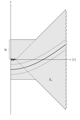
Figure 5.3. A spacetime diagram illustrating the construction of the initial data for the hyperboloidal evolution. The shaded region depicts the domain $\Lambda_{\epsilon}$. The solid curved line represents the hyperboloid parametrized by the map $y\mapsto(T+e^{-s}h(y),e^{-s}y)$ with $T=1$ and $s=\log(-\frac{h(0)}{1+2\epsilon})$. The dotted lines are the corresponding translated hyperboloids with the same $s$ but $T=1-\epsilon$ and $T=1+\epsilon$, respectively. The zigzag segment represents the support of the initial data $(f,g)$.

Consequently, our goal is now to solve Eq. (5.2) for $s\geq s_{0}=\log(-\frac{h(0)}{1+2\epsilon})$ with initial data $\Phi(s_{0})=\mathbf{U}((f,g),T)$ and a suitable $T\in[1-\epsilon,1+\epsilon]$.

5.2. Properties of the initial data operator

First, we prove mapping properties for the initial data operator $\mathbf{U}$.

Lemma 5.5.

Let $R\geq\frac{1}{2}$ and $k\in\mathbb{N}$, $k\geq 4$. Then there exists an $\epsilon>0$ such that the initial data operator $\mathbf{U}:\mathcal{B}^{k+4}_{1,\epsilon}\times[1-\epsilon,1+\epsilon]\to\mathcal{H}_{R}^{k}$ is well-defined and for any $(f,g)\in\mathcal{B}_{1,\epsilon}^{k+4}$, the map $\mathbf{U}((f,g),\cdot):[1-\epsilon,1+\epsilon]\to\mathcal{H}_{R}^{k}$ is continuous. Furthermore, there exists a $\gamma_{\epsilon}\in\mathbb{R}$ such that

$$\mathbf{U}((f,g),T)=\gamma_{\epsilon}(T-1)\mathbf{f}_{1}^{*}+\mathbf{V}((f,g),T),$$

where $\mathbf{V}((f,g),T)$ satisfies the bound

$$\|\mathbf{V}((f,g),T)\|_{\mathcal{H}^{k}_{R}}\lesssim\|(f,g)\|_{H^{k+4}(\mathbb{R}^{5})\times H^{k+3}(\mathbb{R}^{5})}+|T-1|^{2}.$$

Proof.

According to Lemma 5.3, there exists an $\epsilon>0$ such that the operator is well-defined since the hyperboloids on which the function $u_{f,g}$ is evaluated lie entirely inside of $\Lambda_{\epsilon}$, see Fig. 5.3. The statement about the continuity is a simple consequence of the fact that $u_{f,g},u_{T}^{*}\in C^{\infty}(\Lambda_{\epsilon})$. To prove the last assertion, we rewrite $\mathbf{U}$ as

$$\mathbf{U}((f,g),T)(y) =e^{-s}\left.\begin{pmatrix}u_{f,g}(T+e^{-s}h(y),e^{-s}y)-u_{1}^{*}(T+e^{-s}h(y),e^{-s}y)\\ \partial_{s}u_{f,g}(T+e^{-s}h(y),e^{-s}y)-\partial_{s}u_{1}^{*}(T+e^{-s}h(y),e^{-s}y)\end{pmatrix}\right|_{s=\log(-\frac{h(0)}{1+2\epsilon})}$$

$$\quad+e^{-s}\left.\begin{pmatrix}u_{1}^{*}(T+e^{-s}h(y),e^{-s}y)-u_{T}^{*}(T+e^{-s}h(y),e^{-s}y)\\ \partial_{s}u_{1}^{*}(T+e^{-s}h(y),e^{-s}y)-\partial_{s}u_{T}^{*}(T+e^{-s}h(y),e^{-s}y)\end{pmatrix}\right|_{s=\log(-\frac{h(0)}{1+2\epsilon})}.$$

Now note that $u_{T+t_{0}}^{*}(t+t_{0},x)=u_{T}^{*}(t,x)$ for any $t_{0}\in\mathbb{R}$ and thus, by expanding around $T=1$, we infer

$$u_{1}^{*}(T+e^{-s}h(y),e^{-s}y) =u_{2-T}^{*}(1+e^{-s}h(y),e^{-s}y)$$

$$=u_{1}^{*}(1+e^{-s}h(y),e^{-s}y)$$

$$\quad+\partial_{T}u_{2-T}^{*}(1+e^{-s}h(y),e^{-s}y)|_{T=1}(T-1)+\varphi_{T}(s,y),$$

where $\|(\varphi_{T}(s,\cdot),\partial_{s}\varphi_{T}(s,\cdot))\|_{\mathcal{H}_{R}^{k}}\leq C_{s}|T-1|^{2}$. Since

$$\partial_{T}u_{T}^{*}(t,x)=-\frac{2}{(T-t)^{2}+|x|^{2}},$$

see the proof of Lemma 4.4, we obtain

$$\partial_{T}u_{2-T}^{*}(t,x)|_{T=1}=-\partial_{T}u_{T}^{*}(t,x)|_{T=1}=\frac{2}{(1-t)^{2}+|x|^{2}}$$

and thus,

$$u_{1}^{*}(T+e^{-s}h(y),e^{-s}y) =u_{1}^{*}(1+e^{-s}h(y),e^{-s}y)+2\frac{e^{2s}}{|y|^{2}+h(y)^{2}}(T-1)+\varphi_{T}(s,y)$$

$$=u_{T}^{*}(T+e^{-s}h(y),e^{-s}y)+2e^{2s}f_{1,1}^{*}(y)(T-1)+\varphi_{T}(s,y)$$

$$\partial_{s}u_{1}^{*}(T+e^{-s}h(y),e^{-s}y) =\partial_{s}u_{T}^{*}(T+e^{-s}h(y),e^{-s}y)+2e^{2s}f_{1,2}^{*}(y)(T-1)+\partial_{s}\varphi_{T}(s,y).$$

This yields the stated representation. The bound on $\mathbf{V}((f,g),T)$ follows easily by Sobolev embedding and the estimate from Lemma 5.3. ∎

5.3. Hyperboloidal evolution

The last step in the proof of Theorem 1.2 consists of the hyperboloidal evolution.

Proposition 5.6.

Let $R\geq\frac{1}{2}$ and $k\in\mathbb{N}$, $k\geq 4$. Then there exists an $M>0$ and $\delta,\epsilon>0$ such that for any pair $(f,g)\in\mathcal{B}_{\delta/M,\epsilon}^{k+4}$ there exists a $T_{f,g}\in[1-\delta,1+\delta]$ and a unique function $\Phi_{f,g}\in C([s_{0},\infty),\mathcal{H}_{R}^{k})$ that satisfies

$$\Phi_{f,g}(s)=\mathbf{S}(s-s_{0})\mathbf{U}((f,g),T_{f,g})+\int_{s_{0}}^{s}\mathbf{S}(s-s^{\prime})\mathbf{N}(\Phi_{f,g}(s^{\prime}))ds^{\prime},\qquad s_{0}:=\log\left(-\frac{h(0)}{1+2\epsilon}\right)$$

and $\|\Phi_{f,g}(s)\|_{\mathcal{H}^{k}_{R}}\leq\delta e^{-\omega_{0}s}$ for all $s\geq s_{0}$.

Proof.

Let $c,\delta>0$ be as in Proposition 4.12 and choose $\epsilon>0$ so small that $\mathbf{U}:\mathcal{B}_{1,\epsilon}^{k+4}\times[1-\epsilon,1+\epsilon]\to\mathcal{H}_{R}^{k}$ is well-defined, see Lemma 5.5. By choosing $M_{0}\geq 1$ sufficiently large, we obtain $\frac{\delta}{M_{0}}\leq\epsilon$ and Lemma 5.5 yields the bound $\|\mathbf{U}((f,g),T)\|_{\mathcal{H}_{R}^{k}}\leq\frac{\delta}{c}$ for all $(f,g)\in\mathcal{B}_{\delta/M_{0}^{2},\epsilon}^{k+4}$ and $T\in[1-\frac{\delta}{M_{0}},1+\frac{\delta}{M_{0}}]$. Consequently, Proposition 4.12 implies that for any $(f,g)\in\mathcal{B}_{\delta/M_{0}^{2},\epsilon}^{k+4}$ and $T\in[1-\frac{\delta}{M_{0}},1+\frac{\delta}{M_{0}}]$, there exists a unique function $\Phi_{f,g,T}\in C([s_{0},\infty),\mathcal{H}_{R}^{k})$ satisfying

$$\Phi_{f,g,T}(s)=\mathbf{S}(s-s_{0})\left[\mathbf{U}((f,g),T)-\mathbf{C}_{s_{0}}\big{(}\Phi_{f,g,T},\mathbf{U}((f,g),T)\big{)}\right]+\int_{s_{0}}^{s}\mathbf{S}(s-s^{\prime})\mathbf{N}\big{(}\Phi_{f,g,T}(s^{\prime})\big{)}ds^{\prime},$$

where $s_{0}:=\log(-\frac{h(0)}{1+2\epsilon})$. Furthermore, we have the bound $\|\Phi_{f,g,T}(s)\|_{\mathcal{H}_{R}^{k}}\leq\delta e^{-\omega_{0}s}$ for all $s\geq s_{0}$. Thus, our goal is to show that there exists a $T_{f,g}\in[1-\frac{\delta}{M_{0}},1+\frac{\delta}{M_{0}}]$ such that

$$\mathbf{C}_{s_{0}}\big{(}\Phi_{f,g,T_{f,g}},\mathbf{U}((f,g),T_{f,g})\big{)}=\mathbf{0}.$$

To this end, we define a function $\varphi_{f,g}:[1-\frac{\delta}{M_{0}},1+\frac{\delta}{M_{0}}]\to\mathbb{R}$ by

$$\varphi_{f,g}(T):=\Big{(}\mathbf{C}_{s_{0}}\big{(}\Phi_{f,g,T},\mathbf{U}((f,g),T)\big{)}\Big{|}\mathbf{f}_{1}^{*}\Big{)}_{\mathcal{H}_{R}^{k}}.$$

By Proposition 4.12 and Lemma 5.5, $\varphi_{f,g}$ is continuous. Recall that

$$\mathbf{C}_{s_{0}}\big{(}\Phi_{f,g,T},\mathbf{U}((f,g),T)\big{)}=\mathbf{P}\mathbf{U}((f,g),T)+\mathbf{P}\int_{s_{0}}^{\infty}e^{s_{0}-s^{\prime}}\mathbf{N}(\Phi_{f,g,T}(s^{\prime}))ds^{\prime}$$

and from Lemmas 4.10 and 5.5 we see that there exists a nonzero constant $\widetilde{\gamma}_{\epsilon}$ such that

$$\varphi_{f,g}(T)=\widetilde{\gamma}_{\epsilon}(T-1)+\phi_{f,g}(T)$$

with a continuous function $\phi_{f,g}:[1-\frac{\delta}{M_{0}},1+\frac{\delta}{M_{0}}]\to\mathbb{R}$ satisfying $|\phi_{f,g}(T)|\lesssim\frac{\delta}{M_{0}^{2}}+\delta^{2}$ for all $T\in[1-\frac{\delta}{M_{0}},1+\frac{\delta}{M_{0}}]$. Consequently, the condition $\varphi_{f,g}(T)=0$ is equivalent to the fixed point problem $T=1-\widetilde{\gamma}_{\epsilon}^{-1}\phi_{f,g}(T)$ and if we choose $M_{0}$ large enough and $\delta>0$ sufficiently small, $T\mapsto 1-\widetilde{\gamma}_{\epsilon}^{-1}\phi_{f,g}(T)$ becomes a continuous self-map of the interval $[1-\frac{\delta}{M_{0}},1+\frac{\delta}{M_{0}}]$ which necessarily has a fixed point $T_{f,g}$. By Proposition 4.7, $\mathbf{C}_{s_{0}}$ has values in $\langle\mathbf{f}_{1}^{*}\rangle$ and thus,

$$\mathbf{C}_{s_{0}}\big{(}\Phi_{f,g,T_{f,g}},\mathbf{U}((f,g),T_{f,g})\big{)}=\mathbf{0},$$

as desired. The proof is finished by setting $M=M_{0}^{2}$. ∎

5.4. Proof of Theorem 1.2

Let $m\in\mathbb{N}$, $m\geq 8$. According to Lemmas 5.3, 5.5, and Proposition 5.6, there exists an $\epsilon>0$ such that for any pair of functions $(f,g)\in\mathcal{B}_{\delta/M,\epsilon}^{m}$ there exists a $T\in[1-\delta,1+\delta]$ and a continuous function $\Phi=(\phi_{1},\phi_{2}):[s_{0},\infty)\to\mathcal{H}_{R}^{m-4}$ that satisfies

$$\Phi(s)=\mathbf{S}(s-s_{0})\mathbf{U}((f,g),T)+\int_{s_{0}}^{s}\mathbf{S}(s-s^{\prime})\mathbf{N}(\Phi(s^{\prime}))ds^{\prime}$$

for all $s\geq s_{0}:=\log(-\frac{h(0)}{1+2\epsilon})$ and $\|\Phi(s)\|_{\mathcal{H}^{m-4}_{R}}\leq\delta e^{-\omega_{0}s}$. Since the data $\mathbf{U}((f,g),T)$ are smooth, they belong to $\mathcal{D}(\mathbf{L})$ and the function $\Phi$ is a classical solution to the equation

$$\partial_{s}\Phi(s)=\mathbf{L}\Phi(s)+\mathbf{N}(\Phi(s)).$$

By a simple inductive argument it follows that $\Phi$ is in fact smooth, cf. the proof of Theorem 2.14. By construction, the function $u$, given by

$$(u\circ\eta_{T})(s,y)=(u_{T}^{*}\circ\eta_{T})(s,y)+e^{s}\phi_{1}(s)(y),$$

satisfies Eq. (1.5) in the domain $\eta_{T}([s_{0},\infty)\times\mathbb{B}_{R}^{5})$ and we have

$$\partial_{s}(u\circ\eta_{T})(s,y)=\partial_{s}(u_{T}^{*}\circ\eta_{T})(s,y)+e^{s}\phi_{2}(s)(y).$$

By Theorem 2.12 we have $u(0,\cdot)=u_{1}^{*}(0,\cdot)+f$ and $\partial_{0}u(0,\cdot)=\partial_{0}u_{1}^{*}(0,\cdot)+g$ and the stated bounds in Theorem 1.2 follow immediately from

$$\|\Phi(s)\|_{\mathcal{H}_{R}^{m-4}}^{2}=\|\phi_{1}(s)\|_{H^{m-3}(\mathbb{B}_{R}^{5})}^{2}+\|\phi_{2}(s)\|_{H^{m-4}(\mathbb{B}_{R}^{5})}^{2}\leq\delta^{2}e^{-2\omega_{0}s}.$$

Finally, $u=u_{1}^{*}$ in $\Omega_{T,b}\setminus\eta_{T}([s_{0},\infty)\times\mathbb{B}_{R}^{5})$ is a consequence of finite speed of propagation, Theorem 2.12.

Appendix A Technical lemmas

In this section we collect some technical lemmas and elementary estimates. We start with two variants of the classical Hardy inequality in one dimension.

Lemma A.1.

Let $s\in\mathbb{R}\setminus\{-\frac{1}{2}\}$. Then we have the estimate

$$\||\cdot|^{s}f\|_{L^{2}(\mathbb{R})}\lesssim\||\cdot|^{s+1}f^{\prime}\|_{L^{2}(\mathbb{R})}$$

for all $f\in\mathcal{S}(\mathbb{R})$ satisfying

$$\lim_{x\to 0}\left[|x|^{s+\frac{1}{2}}|f(x)|\right]=0.$$

Proof.

For $n\in\mathbb{N}$ we have

$$\int_{\mathbb{R}\setminus\mathbb{B}_{1/n}}|x|^{2s}|f(x)|^{2}dx =\int_{-\infty}^{-1/n}(-x)^{2s}f(x)^{2}dx+\int_{1/n}^{\infty}x^{2s}f(x)^{2}dx$$

$$=-\tfrac{1}{2s+1}(-x)^{2s+1}f(x)^{2}\Big{|}_{-\infty}^{-1/n}+\tfrac{1}{2s+1}x^{2s+1}f(x)^{2}\Big{|}_{1/n}^{\infty}$$

$$\quad+\frac{2}{2s+1}\left[\int_{-\infty}^{-1/n}(-x)^{2s+1}f^{\prime}(x)f(x)dx-\int_{1/n}^{\infty}x^{2s+1}f^{\prime}(x)f(x)dx\right]$$

and Cauchy-Schwarz implies

$$\||\cdot|^{s}f\|_{L^{2}(\mathbb{R}\setminus\mathbb{B}_{1/n})}^{2}\lesssim B_{n}(f)+\||\cdot|^{s}f\|_{L^{2}(\mathbb{R}\setminus\mathbb{B}_{1/n})}\||\cdot|^{s+1}f^{\prime}\|_{L^{2}(\mathbb{R}\setminus\mathbb{B}_{1/n})},$$

where

$$B_{n}(f):=(\tfrac{1}{n})^{2s+1}f(-\tfrac{1}{n})^{2}+(\tfrac{1}{n})^{2s+1}f(\tfrac{1}{n})^{2}.$$

By assumption, $B_{n}(f)\to 0$ as $n\to\infty$ and the $L^{2}$ norms in the above inequality are monotonically increasing functions of $n$. Consequently, we infer

$$\||\cdot|^{s}f\|_{L^{2}(\mathbb{R}\setminus\mathbb{B}_{1/n})} \lesssim\frac{B_{n}(f)}{\||\cdot|^{s}f\|_{L^{2}(\mathbb{R}\setminus\mathbb{B}_{1/n})}}+\||\cdot|^{s+1}f^{\prime}\|_{L^{2}(\mathbb{R}\setminus\mathbb{B}_{1/n})}$$

$$\lesssim\frac{B_{n}(f)}{\||\cdot|^{s}f\|_{L^{2}(\mathbb{R}\setminus\mathbb{B})}}+\||\cdot|^{s+1}f^{\prime}\|_{L^{2}(\mathbb{R}\setminus\mathbb{B}_{1/n})}.$$

Both sides of this inequality have limits in the extended reals $\mathbb{R}\cup\{\infty\}$ and the claim follows by taking $n\to\infty$. ∎

Lemma A.2.

Let $s<-\frac{1}{2}$ and $R>0$. Then we have the estimate

$$\||\cdot|^{s}f\|_{L^{2}(\mathbb{B}_{R})}\lesssim\||\cdot|^{s+1}f^{\prime}\|_{L^{2}(\mathbb{B}_{R})}$$

for all $f\in C^{1}(\overline{\mathbb{B}_{R}})$ satisfying

$$\lim_{x\to 0}\left[|x|^{s+\frac{1}{2}}|f(x)|\right]=0.$$

Proof.

Integration by parts, cf.  the proof of Lemma A.1. ∎

Next, we derive a convenient expression for the $H^{k}(\mathbb{R}^{5})$ norm of a radial function $f\in\mathcal{S}(\mathbb{R}^{5})$ in terms of a weighted $H^{k}(\mathbb{R})$ norm of its representative $\widehat{f}(|x|)=f(x)$.

Lemma A.3.

Let $k\in\mathbb{N}_{0}$. Then we have

$$\|f\|_{H^{k}(\mathbb{R}^{5})}\simeq\||\cdot|^{2}\widehat{f}\|_{H^{k}(\mathbb{R})}$$

for all radial $f\in\mathcal{S}(\mathbb{R}^{5})$, where $f(x)=\widehat{f}(|x|)$.

Proof.

For $k=0$ the statement is trivial. Thus, assume $k\in\mathbb{N}$. Let

$$\mathcal{F}_{d}f(\xi):=\int_{\mathbb{R}^{d}}e^{-i\xi x}f(x)dx$$

denote the Fourier transform in $d$ dimensions. Since $f$ is radial, we have

$$\mathcal{F}_{5}f(\xi)=(2\pi)^{\frac{5}{2}}|\xi|^{-\frac{3}{2}}\int_{0}^{\infty}\widehat{f}(r)J_{3/2}(r|\xi|)r^{\frac{5}{2}}dr,$$

see e.g. [30], p. 577. The Bessel function $J_{3/2}$ can be given in terms of elementary functions and we have

$$J_{3/2}(z)=\sqrt{2}\pi^{-\frac{1}{2}}\left(z^{-\frac{3}{2}}\sin z-z^{-\frac{1}{2}}\cos z\right).$$

Consequently,

$$\mathcal{F}_{5}f(\xi) =8\pi^{2}|\xi|^{-3}\int_{0}^{\infty}\widehat{f}(r)\sin(r|\xi|)rdr-8\pi^{2}|\xi|^{-2}\int_{0}^{\infty}\widehat{f}(r)\cos(r|\xi|)r^{2}dr$$

$$=4i\pi^{2}|\xi|^{-3}\int_{\mathbb{R}}e^{-i|\xi|r}r\widehat{f}(r)dr-4\pi^{2}|\xi|^{-2}\int_{\mathbb{R}}e^{-i|\xi|r}r^{2}\widehat{f}(r)dr$$

$$=4i\pi^{2}|\xi|^{-3}\mathcal{F}_{1}((\cdot)\widehat{f})(|\xi|)-4\pi^{2}|\xi|^{-2}\mathcal{F}_{1}(|\cdot|^{2}\widehat{f})(|\xi|)$$

since $\widehat{f}$ is even. Lemma A.1 now yields

$$\begin{split}\|f\|_{\dot{H}^{k}(\mathbb{R}^{5})}&\simeq\||\cdot|^{k}\mathcal{F}_{5}f\|_{L^{2}(\mathbb{R}^{5})}\lesssim\||\cdot|^{k-1}\mathcal{F}_{1}((\cdot)\widehat{f})\|_{L^{2}(\mathbb{R})}+\||\cdot|^{k}\mathcal{F}_{1}(|\cdot|^{2}\widehat{f})\|_{L^{2}(\mathbb{R})}\\ &\lesssim\||\cdot|^{k}\mathcal{F}_{1}((\cdot)\widehat{f})^{\prime}\|_{L^{2}(\mathbb{R})}+\||\cdot|^{k}\mathcal{F}_{1}(|\cdot|^{2}\widehat{f})\|_{L^{2}(\mathbb{R})}\simeq\||\cdot|^{k}\mathcal{F}_{1}(|\cdot|^{2}\widehat{f})\|_{L^{2}(\mathbb{R})}\\ &\simeq\||\cdot|^{2}\widehat{f}\|_{\dot{H}^{k}(\mathbb{R})}\end{split}$$ (A.1)

and thus,

$$\|f\|_{H^{k}(\mathbb{R}^{5})}\simeq\||\cdot|^{2}\widehat{f}\|_{L^{2}(\mathbb{R})}+\||\cdot|^{2}\widehat{f}\|_{\dot{H}^{k}(\mathbb{R})}\lesssim\||\cdot|^{2}\widehat{f}\|_{H^{k}(\mathbb{R})}.$$

Conversely, we have $\widehat{f}(r)=f(re_{1})$ and thus, $\widehat{f}^{(j)}(r)=\partial_{1}^{j}f(re_{1})$ for all $j\in\mathbb{N}_{0}$. Hardy’s inequality yields

$$\|\widehat{f}\|_{L^{2}(\mathbb{R})} \simeq\||\cdot|^{-2}f\|_{L^{2}(\mathbb{R}^{5})}\lesssim\|f\|_{\dot{H}^{2}(\mathbb{R}^{5})}$$

$$\||\cdot|\widehat{f}^{\prime}\|_{L^{2}(\mathbb{R})} \simeq\||\cdot|^{-1}\partial_{1}f\|_{L^{2}(\mathbb{R}^{5})}\lesssim\|f\|_{\dot{H}^{2}(\mathbb{R}^{5})}$$

$$\||\cdot|^{2}\widehat{f}^{\prime\prime}\|_{L^{2}(\mathbb{R})} \simeq\|\partial_{1}^{2}f\|_{L^{2}(\mathbb{R}^{5})}\lesssim\|f\|_{\dot{H}^{2}(\mathbb{R}^{5})}.$$

These estimates imply $\||\cdot|^{2}\widehat{f}\|_{H^{k}(\mathbb{R})}\lesssim\|f\|_{H^{k}(\mathbb{R}^{5})}$, which finishes the proof. ∎

By a standard extension argument, the same bounds hold on balls.

Lemma A.4.

Fix $R>0$ and $k\in\mathbb{N}_{0}$. Then there exists an extension $\mathcal{E}:C^{k}(\overline{\mathbb{B}_{R}})\to C^{k}(\mathbb{R})$ such that $\mathcal{E}f|_{\mathbb{B}_{R}}=f$, $\mathrm{supp}\,(\mathcal{E}f)\subset\mathbb{B}_{2R}$, and

$$\|\mathcal{E}f\|_{H^{k}(\mathbb{R}\setminus\mathbb{B}_{R})}\lesssim\|f\|_{H^{k}(\mathbb{B}_{R}\setminus\mathbb{B}_{R/2})}$$

for all $f\in C^{k}(\overline{\mathbb{B}_{R}})$.

Proof.

We start with the simplest case $k=0$. Let $\chi:\mathbb{R}\to[0,1]$ be a smooth cut-off satisfying

$$\chi(x)=\begin{cases}1&|x|\leq 1\\ 0&|x|\geq\frac{3}{2}\end{cases}.$$

Then we define

$$\mathcal{E}f(x):=\chi(\tfrac{x}{R})\begin{cases}f(-2R-x)&x<-R\\ f(x)&x\in[-R,R]\\ f(2R-x)&x>R\end{cases}.$$

Evidently, $\mathcal{E}f|_{\mathbb{B}_{R}}=f$, $\mathrm{supp}\,(\mathcal{E}f)\subset\mathbb{B}_{\frac{3}{2}R}\subset\mathbb{B}_{2R}$, and $\mathcal{E}f\in C(\mathbb{R}\setminus\{-R,R\})$. Furthermore,

$$\lim_{x\to-R-}\mathcal{E}f(x) =\chi(-1)f(-R)=f(-R)=\lim_{x\to-R+}f(x)=\lim_{x\to-R+}\mathcal{E}f(x)$$

$$\lim_{x\to R+}\mathcal{E}f(x) =\chi(1)f(R)=f(R)=\lim_{x\to R-}f(x)=\lim_{x\to R-}\mathcal{E}f(x)$$

and thus, $\mathcal{E}f\in C(\mathbb{R})$. Finally,

$$\|\mathcal{E}f\|_{L^{2}(\mathbb{R}\setminus\mathbb{B}_{R})}^{2} =\int_{-\infty}^{-R}|\mathcal{E}f(x)|^{2}dx+\int_{R}^{\infty}|\mathcal{E}f(x)|^{2}dx$$

$$=\int_{-\frac{3}{2}R}^{-R}\chi(\tfrac{x}{R})^{2}|f(-2R-x)|^{2}dx+\int_{R}^{\frac{3}{2}R}\chi(\tfrac{x}{R})^{2}|f(2R-x)|^{2}dx$$

$$\leq\int_{-\frac{3}{2}R}^{-R}|f(-2R-x)|^{2}dx+\int_{R}^{\frac{3}{2}R}|f(2R-x)|^{2}dx$$

$$=\int_{-R}^{-\frac{1}{2}R}|f(x)|^{2}dx+\int_{\frac{1}{2}R}^{R}|f(x)|^{2}dx$$

$$=\|f\|_{L^{2}(\mathbb{B}_{R}\setminus\mathbb{B}_{R/2})}^{2}.$$

Note, however, that in general $\mathcal{E}f\notin C^{1}(\mathbb{R})$ since

$$\lim_{x\to R+}(\mathcal{E}f)^{\prime}(x)=-f^{\prime}(R).$$

Thus, for $k\geq 1$ the above construction needs to be modified slightly. The idea is to add suitable polynomials to compensate for the lack of differentiability at the points $x=-R$ and $x=R$. For instance, in the case $k=1$ we set

$$\mathcal{E}f(x):=\chi(\tfrac{x}{R})\begin{cases}-f(-2R-x)+2f(-R)&x<-R\\ f(x)&x\in[-R,R]\\ -f(2R-x)+2f(R)&x>R\end{cases}.$$

Then $\mathcal{E}f\in C^{1}(\mathbb{R})$. Furthermore, the one-dimensional Sobolev embedding yields the bound $|f(-R)|+|f(R)|\lesssim\|f\|_{H^{1}(\mathbb{B}_{R}\setminus\mathbb{B}_{R/2})}$ and the claimed estimate follows. Similar constructions exist for general $k\in\mathbb{N}$, cf. [21], Lemma B.2. We omit the details. ∎

Corollary A.5.

Fix $R>0$ and $k\in\mathbb{N}$. Then we have

$$\|f\|_{H^{k}(\mathbb{B}^{5}_{R})}\simeq\||\cdot|^{2}\widehat{f}\|_{H^{k}(\mathbb{B}_{R})}$$

for all radial $f\in C^{\infty}(\overline{\mathbb{B}^{5}_{R}})$, where $f(x)=\widehat{f}(|x|)$.

Proof.

Let $\widetilde{\mathcal{E}}f(x):=(\mathcal{E}\widehat{f})(|x|)$, where $\mathcal{E}:C^{k}(\overline{\mathbb{B}_{R}})\to C^{k}(\mathbb{R})$ is an extension as in Lemma A.4. Then, by Lemma A.3,

$$\|f\|_{H^{k}(\mathbb{B}_{R}^{5})} \lesssim\|\widetilde{\mathcal{E}}f\|_{H^{k}(\mathbb{R}^{5})}\simeq\||\cdot|^{2}\mathcal{E}\widehat{f}\|_{H^{k}(\mathbb{R})}\simeq\||\cdot|^{2}\widehat{f}\|_{H^{k}(\mathbb{B}_{R})}+\||\cdot|^{2}\mathcal{E}\widehat{f}\|_{H^{k}(\mathbb{R}\setminus\mathbb{B}_{R})}$$

$$\lesssim\||\cdot|^{2}\widehat{f}\|_{H^{k}(\mathbb{B}_{R})}+\|\widehat{f}\|_{H^{k}(\mathbb{B}_{R}\setminus\mathbb{B}_{R/2})}$$

$$\lesssim\||\cdot|^{2}\widehat{f}\|_{H^{k}(\mathbb{B}_{R})}.$$

Conversely,

$$\||\cdot|^{2}\widehat{f}\|_{H^{k}(\mathbb{B}_{R})} \lesssim\||\cdot|^{2}\mathcal{E}\widehat{f}\|_{H^{k}(\mathbb{R})}\simeq\|\widetilde{\mathcal{E}}f\|_{H^{k}(\mathbb{R}^{5})}\simeq\|f\|_{H^{k}(\mathbb{B}_{R}^{5})}+\|\widetilde{\mathcal{E}}f\|_{H^{k}(\mathbb{R}^{5}\setminus\mathbb{B}_{R}^{5})}$$

$$\lesssim\|f\|_{H^{k}(\mathbb{B}_{R}^{5})}+\|\mathcal{E}\widehat{f}\|_{H^{k}(\mathbb{R}\setminus\mathbb{B}_{R})}\lesssim\|f\|_{H^{k}(\mathbb{B}_{R}^{5})}+\|\widehat{f}\|_{H^{k}(\mathbb{B}_{R}\setminus\mathbb{B}_{R/2})}$$

$$\lesssim\|f\|_{H^{k}(\mathbb{B}_{R}^{5})},$$

again by Lemma A.3. ∎

To conclude this section, we consider a class of integral operators that will appear frequently in the proof of Proposition 3.6.

Lemma A.6.

Let $R>0$, $m,n\in\mathbb{N}_{0}$, and $n+1-m\geq 0$. Furthermore, let $\varphi\in C^{\infty}(\overline{\mathbb{B}_{R}})$ and define $T:C^{\infty}(\overline{\mathbb{B}_{R}})\to C^{\infty}(\overline{\mathbb{B}_{R}})$ by

$$Tf(x):=\frac{1}{x^{m}}\int_{0}^{x}y^{n}\varphi(y)f(y)dy.$$

Then we have the bound

$$\|Tf\|_{H^{k}(\mathbb{B}_{R})}\leq C_{k}\|f\|_{H^{k}(\mathbb{B}_{R})}$$

for all $f\in C^{\infty}(\overline{\mathbb{B}_{R}})$ and $k\in\mathbb{N}_{0}$. In particular, $T$ extends to a bounded operator on $H^{k}(\mathbb{B}_{R})$.

Proof.

For $x\in\overline{\mathbb{B}_{R}}\setminus\{0\}$ we have

$$Tf(x)=\frac{1}{x^{m}}\int_{0}^{x}y^{n}\varphi(y)f(y)dy=x^{n+1-m}\int_{0}^{1}t^{n}\varphi(tx)f(tx)dt$$

and this shows that $T$ maps $C^{\infty}(\overline{\mathbb{B}_{R}})$ to itself. By the Leibniz rule we infer

$$|(Tf)^{(j)}(x)| \leq C_{k}\sum_{\ell=0}^{j}\int_{0}^{1}|f^{(\ell)}(tx)|dt\leq C_{k}\sum_{\ell=0}^{j}\frac{1}{x}\int_{0}^{x}|f^{(\ell)}(y)|dy$$

for all $j=0,1,2,\dots,k$ and $x\in\mathbb{B}_{R}\setminus\{0\}$. Consequently, Lemma A.2 yields the bound

$$\|(Tf)^{(j)}\|_{L^{2}(\mathbb{B}_{R})}\leq C_{k}\sum_{\ell=0}^{j}\|f^{(\ell)}\|_{L^{2}(\mathbb{B}_{R})}\leq C_{k}\|f\|_{H^{k}(\mathbb{B}_{R})}$$

for all $j=0,1,2,\dots,k$. ∎

Appendix B Proof of Proposition 3.6

Recall that $\mathbf{D}_{5}\mathbf{f}=\widehat{\mathbf{D}}_{5}\mathbf{E}_{1}\mathbf{f}$, where $\mathbf{E}_{1}\mathbf{f}(\eta)=\mathbf{f}(\eta e_{1})$ and

$$\widehat{\mathbf{D}}_{5}\begin{pmatrix}\widehat{f}_{1}\\ \widehat{f}_{2}\end{pmatrix}=\begin{pmatrix}a_{11}\widehat{f}_{1}^{\prime}+a_{10}\widehat{f}_{1}+a_{20}\widehat{f}_{2}\\ b_{12}\widehat{f}_{1}^{\prime\prime}+b_{11}\widehat{f}_{1}^{\prime}+b_{10}\widehat{f}_{1}+b_{21}\widehat{f}_{2}^{\prime}+b_{20}\widehat{f}_{2}\end{pmatrix}.$$

In other words,

$$\mathbf{D}_{5}\begin{pmatrix}f_{1}\\ f_{2}\end{pmatrix}(\eta)$$

$$=\begin{pmatrix}a_{11}(\eta)\partial_{1}f_{1}(\eta e_{1})+a_{10}(\eta)f_{1}(\eta e_{1})+a_{20}(\eta)f_{2}(\eta e_{1})\\ b_{12}(\eta)\partial_{1}^{2}f_{1}(\eta e_{1})+b_{11}(\eta)\partial_{1}f_{1}(\eta e_{1})+b_{10}(\eta)f_{1}(\eta e_{1})+b_{21}(\eta)\partial_{1}f_{2}(\eta e_{1})+b_{20}(\eta)f_{2}(\eta e_{1})\end{pmatrix}.$$

The coefficients are of the form

$$a_{11}(\eta) =\eta^{2}\varphi_{\infty}(\eta) a_{10}(\eta) =3\eta a_{20}(\eta) =\eta^{3}\varphi_{\infty}(\eta)$$

$$b_{12}(\eta) =\eta^{3}\varphi_{\infty}(\eta) b_{11}(\eta) =\eta^{2}\varphi_{\infty}(\eta) b_{10}(\eta) =-3\eta$$

$$b_{21}(\eta) =\eta^{2}\varphi_{\infty}(\eta) b_{20}(\eta) =\eta\varphi_{\infty}(\eta),$$

where $\varphi_{\infty}\in C^{\infty}(\mathbb{R})$ denotes a generic smooth and even function with $\varphi_{\infty}(0)\not=0$. From the form of the coefficients it is obvious that $\widehat{\mathbf{D}}_{5}$ maps even functions to odd functions. Our first goal is to prove the bound

$$\|\mathbf{D}_{5}\mathbf{f}\|_{H^{k}(\mathbb{B}_{R})\times H^{k-1}(\mathbb{B}_{R})}\lesssim\|\mathbf{f}\|_{H^{k+1}(\mathbb{B}_{R}^{5})\times H^{k}(\mathbb{B}_{R}^{5})}.$$

By Lemma 2.4 it suffices to show

$$\|\mathbf{D}_{5}\mathbf{f}\|_{H^{k}(\mathbb{R})\times H^{k-1}(\mathbb{R})}\lesssim\|\mathbf{f}\|_{H^{k+1}(\mathbb{R}^{5})\times H^{k}(\mathbb{R}^{5})}$$ (B.1)

and we may assume that the coefficients of $\mathbf{D}_{5}$ have compact support. Hardy’s inequality yields

$$\|[\mathbf{D}_{5}\mathbf{f}]_{1}\|_{L^{2}(\mathbb{R})} \lesssim\||\cdot|^{2}\partial_{1}f_{1}((\cdot)e_{1})\|_{L^{2}(\mathbb{R})}+\||\cdot|f_{1}((\cdot)e_{1})\|_{L^{2}(\mathbb{R})}+\||\cdot|^{2}f_{2}((\cdot)e_{1})\|_{L^{2}(\mathbb{R})}$$

$$\lesssim\|\nabla f_{1}\|_{L^{2}(\mathbb{R}^{5})}+\||\cdot|^{-1}f_{1}\|_{L^{2}(\mathbb{R}^{5})}+\|f_{2}\|_{L^{2}(\mathbb{R}^{5})}$$

$$\lesssim\|f_{1}\|_{H^{1}(\mathbb{R}^{5})}+\|f_{2}\|_{L^{2}(\mathbb{R}^{5})}$$

and from the Leibniz rule we infer $\|[\mathbf{D}_{5}\mathbf{f}]_{1}\|_{H^{k}(\mathbb{R})}\lesssim\|\mathbf{f}\|_{H^{k+1}(\mathbb{R}^{5})\times H^{k}(\mathbb{R}^{5})}$. Analogously, we obtain $\|[\mathbf{D}_{5}\mathbf{f}]_{2}\|_{H^{k-1}(\mathbb{R}^{5})}\lesssim\|\mathbf{f}\|_{H^{k+1}(\mathbb{R}^{5})\times H^{k}(\mathbb{R}^{5})}$ and this proves Eq. (B.1).

Thus, it remains to show the more difficult reverse inequality

$$\|\mathbf{D}_{5}\mathbf{f}\|_{H^{k}(\mathbb{B}_{R})\times H^{k-1}(\mathbb{B}_{R})}\gtrsim\|\mathbf{f}\|_{H^{k+1}(\mathbb{B}^{5}_{R})\times H^{k}(\mathbb{B}^{5}_{R})}$$

or, by Corollary A.5, the equivalent estimate

$$\left\|\widehat{\mathbf{D}}_{5}\widehat{\mathbf{f}}\right\|_{H^{k}(\mathbb{B}_{R})\times H^{k-1}(\mathbb{B}_{R})}\gtrsim\left\||\cdot|^{2}\,\widehat{\mathbf{f}}\right\|_{H^{k+1}(\mathbb{B}_{R})\times H^{k}(\mathbb{B}_{R})}.$$ (B.2)

Let $\mathbf{g}:=\widehat{\mathbf{D}}_{5}\widehat{\mathbf{f}}$. Then we have

$$g_{1} =a_{11}\widehat{f}_{1}^{\prime}+a_{10}\widehat{f}_{1}+a_{20}\widehat{f}_{2}$$

$$g_{2} =b_{12}\widehat{f}_{1}^{\prime\prime}+b_{11}\widehat{f}_{1}^{\prime}+b_{10}\widehat{f}_{1}+b_{21}\widehat{f}_{2}^{\prime}+b_{20}\widehat{f}_{2}.$$

We use the first equation to eliminate $\widehat{f}_{2}$ from the second equation. This yields

$$\widehat{f}_{1}^{\prime\prime}(\eta)+\left(\frac{6}{\eta}-\frac{h^{\prime\prime}(\eta)}{h^{\prime}(\eta)}\right)\widehat{f}_{1}^{\prime}(\eta)+3\frac{2h^{\prime}(\eta)-\eta h^{\prime\prime}(\eta)}{\eta^{2}h^{\prime}(\eta)}\widehat{f}_{1}(\eta)=\frac{a(\eta)}{\eta^{2}}g_{1}^{\prime}(\eta)+\frac{b(\eta)}{\eta}g_{2}(\eta),$$ (B.3)

where

$$a(\eta) =\frac{2\eta h^{\prime}(\eta)-h(\eta)[1+h^{\prime}(\eta)^{2}]}{\eta h^{\prime}(\eta)-h(\eta)}, b(\eta) =\frac{h^{\prime}(\eta)}{\eta}\frac{1-h^{\prime}(\eta)^{2}}{\eta h^{\prime}(\eta)-h(\eta)}.$$

Note that $a,b\in C^{\infty}(\mathbb{R})$ are even and $a(0)\not=0$, $b(0)\not=0$. If $g_{1}=g_{2}=0$, Eq. (B.3) has the two solutions

$$\phi(\eta)=\frac{\sqrt{2+\eta^{2}}-\sqrt{2}}{\eta^{3}}=\frac{\varphi_{\infty}(\eta)}{\eta},\qquad\psi(\eta)=\frac{1}{\eta^{3}}$$

with Wronskian

$$W(\eta)=\phi(\eta)\psi^{\prime}(\eta)-\phi^{\prime}(\eta)\psi(\eta)=-\frac{1}{\eta^{5}\sqrt{2+\eta^{2}}}.$$

Consequently, the variation of constants formula yields

$$\widehat{f}_{1}(\eta)=c_{0}\phi(\eta)+c_{1}\psi(\eta)-\phi(\eta)\int_{0}^{\eta}\frac{\psi(\eta^{\prime})}{W(\eta^{\prime})}g(\eta^{\prime})d\eta^{\prime}+\psi(\eta)\int_{0}^{\eta}\frac{\phi(\eta^{\prime})}{W(\eta^{\prime})}g(\eta^{\prime})d\eta^{\prime}$$

where $c_{0},c_{1}\in\mathbb{R}$ and $g$ denotes the right-hand side of Eq. (B.3). Since $f_{1}(y)=\widehat{f}_{1}(|y|)$ belongs to $H^{3}(\mathbb{B}_{R}^{5})$, it follows that $c_{0}=c_{1}=0$. In particular, this shows that the map $\mathbf{D}_{5}:H^{k+1}_{\mathrm{rad}}(\mathbb{B}_{R}^{5})\times H^{k}_{\mathrm{rad}}(\mathbb{B}_{R}^{5})\to H_{-}^{k}(\mathbb{B}_{R})\times H_{-}^{k-1}(\mathbb{B}_{R})$ is injective. Thus, we have $\widehat{f}_{1}=T_{1}g_{1}+T_{2}g_{2}$, where

$$T_{1}g_{1}(\eta) :=\psi(\eta)\int_{0}^{\eta}\frac{\phi(\eta^{\prime})a(\eta^{\prime})}{\eta^{\prime 2}W(\eta^{\prime})}g_{1}^{\prime}(\eta^{\prime})d\eta^{\prime}-\phi(\eta)\int_{0}^{\eta}\frac{\psi(\eta^{\prime})a(\eta^{\prime})}{\eta^{\prime 2}W(\eta^{\prime})}g_{1}^{\prime}(\eta^{\prime})d\eta^{\prime}$$

$$T_{2}g_{2}(\eta) :=\psi(\eta)\int_{0}^{\eta}\frac{\phi(\eta^{\prime})b(\eta^{\prime})}{\eta^{\prime}W(\eta^{\prime})}g_{2}(\eta^{\prime})d\eta^{\prime}-\phi(\eta)\int_{0}^{\eta}\frac{\psi(\eta^{\prime})b(\eta^{\prime})}{\eta^{\prime}W(\eta^{\prime})}g_{2}(\eta^{\prime})d\eta^{\prime}.$$

In view of Corollary A.5, we have to prove the bounds

$$\||\cdot|^{2}T_{1}g_{1}\|_{H^{k+1}(\mathbb{B}_{R})} \lesssim\|g_{1}\|_{H^{k}(\mathbb{B}_{R})}$$

$$\||\cdot|^{2}T_{2}g_{2}\|_{H^{k+1}(\mathbb{B}_{R})} \lesssim\|g_{2}\|_{H^{k-1}(\mathbb{B}_{R})}.$$

An integration by parts using $g_{1}(0)=0$ yields

$$\begin{split}T_{1}g_{1}(\eta)&=\phi(\eta)\int_{0}^{\eta}\partial_{\eta^{\prime}}\left[\frac{\psi(\eta^{\prime})a(\eta^{\prime})}{\eta^{\prime 2}W(\eta^{\prime})}\right]g_{1}(\eta^{\prime})d\eta^{\prime}-\psi(\eta)\int_{0}^{\eta}\partial_{\eta^{\prime}}\left[\frac{\phi(\eta^{\prime})a(\eta^{\prime})}{\eta^{\prime 2}W(\eta^{\prime})}\right]g_{1}(\eta^{\prime})d\eta^{\prime}\\ &=\frac{\varphi_{\infty}(\eta)}{\eta}\int_{0}^{\eta}\eta^{\prime}\varphi_{\infty}(\eta^{\prime})g_{1}(\eta^{\prime})d\eta^{\prime}+\frac{\varphi_{\infty}(\eta)}{\eta^{3}}\int_{0}^{\eta}\eta^{\prime}\varphi_{\infty}(\eta^{\prime})g_{1}(\eta^{\prime})d\eta^{\prime}\end{split}$$ (B.4)

and for brevity we set

$$T_{11}g_{1}(\eta) :=\frac{\varphi_{\infty}(\eta)}{\eta}\int_{0}^{\eta}\eta^{\prime}\varphi_{\infty}(\eta^{\prime})g_{1}(\eta^{\prime})d\eta^{\prime}$$

$$T_{12}g_{1}(\eta) :=\frac{\varphi_{\infty}(\eta)}{\eta^{3}}\int_{0}^{\eta}\eta^{\prime}\varphi_{\infty}(\eta^{\prime})g_{1}(\eta^{\prime})d\eta^{\prime}.$$

By Lemma A.6 we immediately obtain the bound $\||\cdot|^{2}T_{11}g_{1}\|_{L^{2}(\mathbb{B}_{R})}\lesssim\|g_{1}\|_{L^{2}(\mathbb{B}_{R})}$ and, since

$$\partial_{\eta}\left[\eta^{2}T_{11}g_{1}(\eta)\right]=\varphi_{\infty}(\eta)\int_{0}^{\eta}\eta^{\prime}\varphi_{\infty}(\eta^{\prime})g_{1}(\eta^{\prime})d\eta^{\prime}+\eta^{2}\varphi_{\infty}(\eta)g_{1}(\eta),$$

we infer $\||\cdot|^{2}T_{11}g_{1}\|_{H^{k+1}(\mathbb{B}_{R})}\lesssim\|g_{1}\|_{H^{k}(\mathbb{B}_{R})}$. Similarly, since

$$\eta^{2}T_{12}g_{1}(\eta)=\frac{\varphi_{\infty}(\eta)}{\eta}\int_{0}^{\eta}\eta^{\prime}\varphi_{\infty}(\eta^{\prime})g_{1}(\eta^{\prime})d\eta^{\prime}$$

and

$$\partial_{\eta}[\eta^{2}T_{12}g_{1}(\eta)] =\frac{\varphi_{\infty}(\eta)}{\eta^{2}}\int_{0}^{\eta}\eta^{\prime}\varphi_{\infty}(\eta^{\prime})g_{1}(\eta^{\prime})d\eta^{\prime}+\varphi_{\infty}(\eta)g_{1}(\eta),$$

Lemma A.6 yields $\|T_{12}g_{1}\|_{H^{k+1}(\mathbb{B}_{R})}\lesssim\|g_{1}\|_{H^{k}(\mathbb{B}_{R})}$. Next, we turn to the operator $T_{2}$. We have

$$\eta^{2}T_{2}g_{2}(\eta)=\frac{\varphi_{\infty}(\eta)}{\eta}\int_{0}^{\eta}\eta^{\prime 3}\varphi_{\infty}(\eta^{\prime})g_{2}(\eta^{\prime})d\eta^{\prime}+\eta\varphi_{\infty}(\eta)\int_{0}^{\eta}\eta^{\prime}\varphi_{\infty}(\eta^{\prime})g_{2}(\eta^{\prime})d\eta^{\prime}$$

and Lemma A.6 immediately yields the bound $\||\cdot|^{2}T_{2}g_{2}\|_{L^{2}(\mathbb{B}_{R})}\lesssim\|g_{2}\|_{L^{2}(\mathbb{B}_{R})}$. Now we exploit the usual cancellation to obtain

$$(T_{2}g_{2})^{\prime}(\eta) =\psi^{\prime}(\eta)\int_{0}^{\eta}\frac{\phi(\eta^{\prime})b(\eta^{\prime})}{\eta^{\prime}W(\eta^{\prime})}g_{2}(\eta^{\prime})d\eta^{\prime}-\phi^{\prime}(\eta)\int_{0}^{\eta}\frac{\psi(\eta^{\prime})b(\eta^{\prime})}{\eta^{\prime}W(\eta^{\prime})}g_{2}(\eta^{\prime})d\eta^{\prime}$$

$$=\frac{\varphi_{\infty}(\eta)}{\eta^{4}}\int_{0}^{\eta}\eta^{\prime 3}\varphi_{\infty}(\eta^{\prime})g_{2}(\eta^{\prime})d\eta^{\prime}+\frac{\varphi_{\infty}(\eta)}{\eta^{2}}\int_{0}^{\eta}\eta^{\prime}\varphi_{\infty}(\eta^{\prime})g_{2}(\eta^{\prime})d\eta^{\prime}$$

and thus,

$$\partial_{\eta}\left[\eta^{2}(T_{2}g_{2})^{\prime}(\eta)\right] =\frac{\varphi_{\infty}(\eta)}{\eta^{3}}\int_{0}^{\eta}\eta^{\prime 3}\varphi_{\infty}(\eta^{\prime})g_{2}(\eta^{\prime})d\eta^{\prime}$$

$$\quad+\eta\varphi_{\infty}(\eta)\int_{0}^{\eta}\eta^{\prime}\varphi_{\infty}(\eta^{\prime})g_{2}(\eta^{\prime})d\eta^{\prime}+\eta\varphi_{\infty}(\eta)g_{2}(\eta),$$

which yields the bound $\||\cdot|^{2}(T_{2}g_{2})^{\prime}\|_{H^{k}(\mathbb{B}_{R})}\lesssim\|g_{2}\|_{H^{k-1}(\mathbb{B}_{R})}$ by Lemma A.6. Analogously, we infer $\|(\cdot)T_{2}g_{2}\|_{H^{k}(\mathbb{B}_{R})}\lesssim\|g_{2}\|_{H^{k-1}(\mathbb{B}_{R})}$ and in summary,

$$\||\cdot|^{2}T_{2}g_{2}\|_{H^{k+1}(\mathbb{B}_{R})} \lesssim\||\cdot|^{2}T_{2}g_{2}\|_{L^{2}(\mathbb{B}_{R})}+\||\cdot|^{2}(T_{2}g_{2})^{\prime}\|_{H^{k}(\mathbb{B}_{R})}+\|(\cdot)T_{2}g_{2}\|_{H^{k}(\mathbb{B}_{R})}$$

$$\lesssim\|g_{2}\|_{H^{k-1}(\mathbb{B}_{R})},$$

as desired.

Finally, we turn to $\widehat{f}_{2}$, which is given by

$$\widehat{f}_{2} =\frac{g_{1}}{a_{20}}-\frac{a_{11}}{a_{20}}\widehat{f}_{1}^{\prime}-\frac{a_{10}}{a_{20}}\widehat{f}_{1}=S_{1}g_{1}+S_{2}g_{2},$$

where

$$S_{1}g_{1} :=\frac{g_{1}}{a_{20}}-\frac{a_{11}}{a_{20}}(T_{1}g_{1})^{\prime}-\frac{a_{10}}{a_{20}}T_{1}g_{1}$$

$$S_{2}g_{2} :=-\frac{a_{11}}{a_{20}}(T_{2}g_{2})^{\prime}-\frac{a_{10}}{a_{20}}T_{2}g_{2}.$$

We have to show the bounds

$$\||\cdot|^{2}S_{1}g_{1}\|_{H^{k}(\mathbb{B}_{R})} \lesssim\|g_{1}\|_{H^{k}(\mathbb{B}_{R})}$$

$$\||\cdot|^{2}S_{2}g_{2}\|_{H^{k}(\mathbb{B}_{R})} \lesssim\|g_{2}\|_{H^{k-1}(\mathbb{B}_{R})}.$$

For the bound on $S_{1}$ we exploit some subtle cancellations. From Eq. (B.4) we obtain

$$(T_{1}g_{1})^{\prime}(\eta) =\left[\phi(\eta)\partial_{\eta}\frac{\psi(\eta)a(\eta)}{\eta^{2}W(\eta)}-\psi(\eta)\partial_{\eta}\frac{\phi(\eta)a(\eta)}{\eta^{2}W(\eta)}\right]g_{1}(\eta)$$

$$\quad+\phi^{\prime}(\eta)\int_{0}^{\eta}\partial_{\eta^{\prime}}\left[\frac{\psi(\eta^{\prime})a(\eta^{\prime})}{\eta^{\prime 2}W(\eta^{\prime})}\right]g_{1}(\eta^{\prime})d\eta^{\prime}-\psi^{\prime}(\eta)\int_{0}^{\eta}\partial_{\eta^{\prime}}\left[\frac{\phi(\eta^{\prime})a(\eta^{\prime})}{\eta^{\prime 2}W(\eta^{\prime})}\right]g_{1}(\eta^{\prime})d\eta^{\prime}$$

$$=\left[\frac{1}{\eta^{2}}+\varphi_{\infty}(\eta)\right]g_{1}(\eta)$$

$$\quad+\phi^{\prime}(\eta)\int_{0}^{\eta}\partial_{\eta^{\prime}}\left[\frac{\psi(\eta^{\prime})a(\eta^{\prime})}{\eta^{\prime 2}W(\eta^{\prime})}\right]g_{1}(\eta^{\prime})d\eta^{\prime}-\psi^{\prime}(\eta)\int_{0}^{\eta}\partial_{\eta^{\prime}}\left[\frac{\phi(\eta^{\prime})a(\eta^{\prime})}{\eta^{\prime 2}W(\eta^{\prime})}\right]g_{1}(\eta^{\prime})d\eta^{\prime}$$

and thus,

$$a_{20}(\eta)S_{1}g_{1}(\eta) =\left[1-\frac{a_{11}(\eta)}{\eta^{2}}+\eta^{2}\varphi_{\infty}(\eta)\right]g_{1}(\eta)$$

$$\quad-\left[a_{11}(\eta)\phi^{\prime}(\eta)+a_{10}(\eta)\phi(\eta)\right]\int_{0}^{\eta}\partial_{\eta^{\prime}}\left[\frac{\psi(\eta^{\prime})a(\eta^{\prime})}{\eta^{\prime 2}W(\eta^{\prime})}\right]g_{1}(\eta^{\prime})d\eta^{\prime}$$

$$\quad+\left[a_{11}(\eta)\psi^{\prime}(\eta)+a_{10}(\eta)\psi(\eta)\right]\int_{0}^{\eta}\partial_{\eta^{\prime}}\left[\frac{\phi(\eta^{\prime})a(\eta^{\prime})}{\eta^{\prime 2}W(\eta^{\prime})}\right]g_{1}(\eta^{\prime})d\eta^{\prime}$$

$$=\eta^{2}\varphi_{\infty}(\eta)g_{1}(\eta)+\varphi_{\infty}(\eta)\int_{0}^{\eta}\eta^{\prime}\varphi_{\infty}(\eta^{\prime})g_{1}(\eta^{\prime})d\eta^{\prime}$$

since $a_{11}(\eta)\psi^{\prime}(\eta)+a_{10}(\eta)\psi(\eta)=\varphi_{\infty}(\eta)$. We have $|\frac{a_{20}(\eta)}{\eta^{3}}|\gtrsim 1$ for all $\eta\in\mathbb{B}_{R}$ which implies

$$S_{1}g_{1}(\eta)=\frac{\varphi_{\infty}(\eta)}{\eta}g_{1}(\eta)+\frac{\varphi_{\infty}(\eta)}{\eta^{3}}\int_{0}^{\eta}\eta^{\prime}\varphi_{\infty}(\eta^{\prime})g_{1}(\eta^{\prime})d\eta^{\prime}$$

and Lemma A.6 yields the desired bound $\||\cdot|^{2}S_{1}g_{1}\|_{H^{k}(\mathbb{B}_{R})}\lesssim\|g_{1}\|_{H^{k}(\mathbb{B}_{R})}$. Similarly, we have

$$a_{20}(\eta)S_{2}g_{2}(\eta) =-a_{11}(\eta)(T_{2}g_{2})^{\prime}(\eta)-a_{10}(\eta)T_{2}g_{2}(\eta)$$

$$=\left[a_{11}(\eta)\phi^{\prime}(\eta)+a_{10}(\eta)\phi(\eta)\right]\int_{0}^{\eta}\frac{\psi(\eta^{\prime})b(\eta^{\prime})}{\eta^{\prime}W(\eta^{\prime})}g_{2}(\eta^{\prime})d\eta^{\prime}$$

$$\quad-\left[a_{11}(\eta)\psi^{\prime}(\eta)+a_{10}(\eta)\psi(\eta)\right]\int_{0}^{\eta}\frac{\phi(\eta^{\prime})b(\eta^{\prime})}{\eta^{\prime}W(\eta^{\prime})}g_{2}(\eta^{\prime})d\eta^{\prime}$$

$$=\varphi_{\infty}(\eta)\int_{0}^{\eta}\eta^{\prime}\varphi_{\infty}(\eta^{\prime})g_{2}(\eta^{\prime})d\eta^{\prime}+\varphi_{\infty}(\eta)\int_{0}^{\eta}\eta^{\prime 3}\varphi_{\infty}(\eta^{\prime})g_{2}(\eta^{\prime})d\eta^{\prime}$$

and thus,

$$S_{2}g_{2}(\eta)=\frac{\varphi_{\infty}(\eta)}{\eta^{3}}\int_{0}^{\eta}\eta^{\prime}\varphi_{\infty}(\eta^{\prime})g_{2}(\eta^{\prime})d\eta^{\prime}+\frac{\varphi_{\infty}(\eta)}{\eta^{3}}\int_{0}^{\eta}\eta^{\prime 3}\varphi_{\infty}(\eta^{\prime})g_{2}(\eta^{\prime})d\eta^{\prime}.$$

From Lemma A.6 we infer the bound $\||\cdot|^{2}S_{2}g_{2}\|_{L^{2}(\mathbb{B}_{R})}\lesssim\|g_{2}\|_{L^{2}(\mathbb{B}_{R})}$ and

$$\partial_{\eta}\left[\eta^{2}S_{2}g_{2}(\eta)\right] =\frac{\varphi_{\infty}(\eta)}{\eta^{2}}\int_{0}^{\eta}\eta^{\prime}\varphi_{\infty}(\eta^{\prime})g_{2}(\eta^{\prime})d\eta^{\prime}+\varphi_{\infty}(\eta)g_{2}(\eta)$$

yields $\||\cdot|^{2}S_{2}g_{2}\|_{H^{k}(\mathbb{B}_{R})}\lesssim\|g_{2}\|_{H^{k-1}(\mathbb{B}_{R})}$, again by Lemma A.6.

Appendix C A monotonicity formula for the free wave equation

In this section we prove a version of the energy identity that is used for finite speed of propagation.

Lemma C.1.

Let $f\in C^{1}(\overline{\mathbb{B}^{d}})$ and $d\in\mathbb{N}$. Then we have

$$\int_{\mathbb{B}^{d}}f(x)x^{j}\partial_{x^{j}}f(x)dx=-\frac{d}{2}\int_{\mathbb{B}^{d}}f(x)^{2}dx+\frac{1}{2}\int_{\mathbb{S}^{d-1}}f(\omega)^{2}d\sigma(\omega).$$

Proof.

The chain rule yields

$$\partial_{x^{j}}\left[x^{j}f(x)^{2}\right]=df(x)^{2}+2f(x)x^{j}\partial_{x^{j}}f(x)$$

and thus, from the divergence theorem we infer

$$\int_{\mathbb{B}^{d}}f(x)x^{j}\partial_{x^{j}}f(x)dx =-\frac{d}{2}\int_{\mathbb{B}^{d}}f(x)^{2}dx+\frac{1}{2}\int_{\mathbb{B}^{d}}\partial_{x^{j}}\left[x^{j}f(x)^{2}\right]dx$$

$$=-\frac{d}{2}\int_{\mathbb{B}^{d}}f(x)^{2}dx+\frac{1}{2}\int_{\partial\mathbb{B}^{d}}\omega_{j}\omega^{j}f(\omega)^{2}d\sigma(\omega).$$

∎

Lemma C.2.

Let $d\geq 3$ and $T>0$. For $u\in C^{2}(\mathbb{R}^{1,d})$ and $t\in[0,T)$ set

$$E_{u}(t):=\int_{\mathbb{B}_{T-t}^{d}}\partial_{0}u(t,x)^{2}dx+\int_{\mathbb{B}_{T-t}^{d}}\partial^{j}u(t,x)\partial_{j}u(t,x)dx+\frac{1}{T-t}\int_{\partial\mathbb{B}^{d}_{T-t}}u(t,\omega)^{2}d\sigma(\omega).$$

If $\partial^{\mu}\partial_{\mu}u=0$, the function $E_{u}:[0,T)\to[0,\infty)$ is monotonically decreasing.

Proof.

We write $E_{u}=E^{0}_{u}+E^{1}_{u}+B_{u}$, where

$$E^{0}_{u}(t) =\int_{\mathbb{B}_{T-t}^{d}}\partial_{0}u(t,x)^{2}dx=(T-t)^{d}\int_{\mathbb{B}^{d}}\partial_{0}u(t,(T-t)x)^{2}dx$$

$$E^{1}_{u}(t) =\int_{\mathbb{B}_{T-t}^{d}}\partial^{j}u(t,x)\partial_{j}u(t,x)dx=(T-t)^{d}\int_{\mathbb{B}^{d}}\partial^{j}u(t,(T-t)x)\partial_{j}u(t,(T-t)x)dx$$

$$B_{u}(t) =\frac{1}{T-t}\int_{\partial\mathbb{B}^{d}_{T-t}}u(t,\omega)^{2}d\sigma(\omega)=(T-t)^{d-2}\int_{\mathbb{S}^{d-1}}u(t,(T-t)\omega)^{2}d\sigma(\omega).$$

Using Lemma C.1, we compute

$$\frac{d}{dt}E_{u}^{0}(t) =-\frac{d}{T-t}E_{u}^{0}(t)$$

$$\quad+2(T-t)^{d}\int_{\mathbb{B}^{d}}\partial_{0}u(t,(T-t)x)\left[\partial_{0}^{2}u(t,(T-t)x)-x^{j}\partial_{j}\partial_{0}u(t,(T-t)x)\right]dx$$

$$=-\frac{d}{T-t}E_{u}^{0}(t)+2(T-t)^{d}\int_{\mathbb{B}^{d}}\partial_{0}u(t,(T-t)x)\partial_{0}^{2}u(t,(T-t)x)dx$$

$$\quad-2(T-t)^{d-1}\int_{\mathbb{B}^{d}}\partial_{0}u(t,(T-t)x)x^{j}\partial_{x^{j}}\partial_{0}u(t,(T-t)x)dx$$

$$=-\frac{d}{T-t}E_{u}^{0}(t)+2(T-t)^{d}\int_{\mathbb{B}^{d}}\partial_{0}u(t,(T-t)x)\partial_{0}^{2}u(t,(T-t)x)dx$$

$$\quad+d(T-t)^{d-1}\int_{\mathbb{B}^{d}}\partial_{0}u(t,(T-t)x)^{2}dx-(T-t)^{d-1}\int_{\mathbb{S}^{d-1}}\partial_{0}u(t,(T-t)\omega)^{2}d\sigma(\omega)$$

and thus,

$$\frac{d}{dt}E_{u}^{0}(t) =2\int_{\mathbb{B}^{d}_{T-t}}\partial_{0}u(t,x)\partial_{0}^{2}u(t,x)dx-\int_{\partial\mathbb{B}^{d}_{T-t}}\partial_{0}u(t,\omega)^{2}d\sigma(\omega).$$

Analogously, we obtain

$$\frac{d}{dt}E_{u}^{1}(t)=2\int_{\mathbb{B}^{d}_{T-t}}\partial^{j}u(t,x)\partial_{j}\partial_{0}u(t,x)dx-\int_{\partial\mathbb{B}^{d}_{T-t}}\partial^{j}u(t,\omega)\partial_{j}u(t,\omega)d\sigma(\omega)$$

and an integration by parts yields

$$\frac{d}{dt}E_{u}^{1}(t) =-2\int_{\mathbb{B}^{d}_{T-t}}\partial^{j}\partial_{j}u(t,x)\partial_{0}u(t,x)dx+2\int_{\partial\mathbb{B}^{d}_{T-t}}\frac{\omega^{j}}{|\omega|}\partial_{j}u(t,\omega)\partial_{0}u(t,\omega)d\sigma(\omega)$$

$$\quad-\int_{\partial\mathbb{B}^{d}_{T-t}}\partial^{j}u(t,\omega)\partial_{j}u(t,\omega)d\sigma(\omega).$$

Finally,

$$\frac{d}{dt}B_{u}(t) =-\frac{d-2}{T-t}B_{u}(t)$$

$$\quad+2(T-t)^{d-2}\int_{\mathbb{S}^{d-1}}u(t,(T-t)\omega)\left[\partial_{0}u(t,(T-t)\omega)-\omega^{j}\partial_{j}u(t,(T-t)\omega)\right]d\sigma(\omega)$$

$$=-\frac{d-2}{(T-t)^{2}}\int_{\partial\mathbb{B}^{d}_{T-t}}u(t,\omega)^{2}d\sigma(\omega)+\frac{2}{T-t}\int_{\partial\mathbb{B}_{T-t}^{d}}u(t,\omega)\partial_{0}u(t,\omega)d\sigma(\omega)$$

$$\quad-\frac{2}{(T-t)^{2}}\int_{\partial\mathbb{B}_{T-t}^{d}}\omega^{j}\partial_{j}u(t,\omega)u(t,\omega)d\sigma(\omega).$$

In summary, since $\partial_{0}^{2}u-\partial^{j}\partial_{j}u=0$, we infer

$$\frac{d}{dt}E_{u}(t)=\frac{d}{dt}E_{u}^{0}(t)+\frac{d}{dt}E_{u}^{1}(t)+\frac{d}{dt}B_{u}(t)=\int_{\partial\mathbb{B}_{T-t}^{d}}A_{u}(t,\omega)d\sigma(\omega),$$

where

$$A_{u}(t,\omega) =-\partial_{0}u(t,\omega)^{2}-\partial^{j}u(t,\omega)\partial_{j}u(t,\omega)-(d-2)\frac{u(t,\omega)^{2}}{(T-t)^{2}}$$

$$\quad+2\frac{\omega^{j}}{|\omega|}\partial_{j}u(t,\omega)\partial_{0}u(t,\omega)+2\partial_{0}u(t,\omega)\frac{u(t,\omega)}{T-t}-2\frac{\omega^{j}}{|\omega|}\partial_{j}u(t,\omega)\frac{u(t,\omega)}{T-t}.$$

Since $d\geq 3$ we obtain

$$A_{u}(t,\omega) =-\left[\partial_{0}u(t,\omega)-\frac{u(t,\omega)}{T-t}\right]^{2}-\partial^{j}u(t,\omega)\partial_{j}u(t,\omega)-(d-3)\frac{u(t,\omega)^{2}}{(T-t)^{2}}$$

$$\quad+2\frac{\omega^{j}}{|\omega|}\partial_{j}u(t,\omega)\left[\partial_{0}u(t,\omega)-\frac{u(t,\omega)}{T-t}\right]$$

$$\leq 0$$

for all $t\in[0,T)$ and $\omega\in\partial\mathbb{B}_{T-t}^{d}$ by Cauchy’s inequality. ∎

References

- [1] Robert A. Adams and John J. F. Fournier. Sobolev spaces, volume 140 of Pure and Applied Mathematics (Amsterdam). Elsevier/Academic Press, Amsterdam, second edition, 2003.
- [2] Paweł Biernat, Piotr Bizoń, and Maciej Maliborski. Threshold for blowup for equivariant wave maps in higher dimensions. Nonlinearity, 30(4):1513–1522, 2017.
- [3] Piotr Bizoń. Equivariant self-similar wave maps from Minkowski spacetime into 3-sphere. Comm. Math. Phys., 215(1):45–56, 2000.
- [4] Piotr Bizoń and Paweł Biernat. Generic self-similar blowup for equivariant wave maps and Yang-Mills fields in higher dimensions. Comm. Math. Phys., 338(3):1443–1450, 2015.
- [5] Piotr Bizoń, Tadeusz Chmaj, and Zbisław Tabor. Formation of singularities for equivariant -dimensional wave maps into the 2-sphere. Nonlinearity, 14(5):1041–1053, 2001.
- [6] Thierry Cazenave, Jalal Shatah, and A. Shadi Tahvildar-Zadeh. Harmonic maps of the hyperbolic space and development of singularities in wave maps and Yang-Mills fields. Ann. Inst. H. Poincaré Phys. Théor., 68(3):315–349, 1998.
- [7] Athanasios Chatzikaleas, Roland Donninger, and Irfan Glogić. On blowup of co-rotational wave maps in odd space dimensions. J. Differential Equations, 263(8):5090–5119, 2017.
- [8] Elisabetta Chiodaroli and Joachim Krieger. A class of large global solutions for the wave-map equation. Trans. Amer. Math. Soc., 369(4):2747–2773, 2017.
- [9] O. Costin, R. Donninger, and X. Xia. A proof for the mode stability of a self-similar wave map. Nonlinearity, 29(8):2451–2473, 2016.
- [10] Ovidiu Costin, Roland Donninger, and Irfan Glogić. Mode Stability of Self-Similar Wave Maps in Higher Dimensions. Comm. Math. Phys., 351(3):959–972, 2017.
- [11] R. Côte. On the soliton resolution for equivariant wave maps to the sphere. Comm. Pure Appl. Math., 68(11):1946–2004, 2015.
- [12] R. Côte, C. E. Kenig, A. Lawrie, and W. Schlag. Characterization of large energy solutions of the equivariant wave map problem: I. Amer. J. Math., 137(1):139–207, 2015.
- [13] R. Côte, C. E. Kenig, A. Lawrie, and W. Schlag. Characterization of large energy solutions of the equivariant wave map problem: II. Amer. J. Math., 137(1):209–250, 2015.
- [14] Benjamin Dodson and Andrew Lawrie. Scattering for radial, semi-linear, super-critical wave equations with bounded critical norm. Arch. Ration. Mech. Anal., 218(3):1459–1529, 2015.
- [15] Roland Donninger. On stable self-similar blowup for equivariant wave maps. Comm. Pure Appl. Math., 64(8):1095–1147, 2011.
- [16] Roland Donninger. Stable self-similar blowup in energy supercritical Yang-Mills theory. Math. Z., 278(3-4):1005–1032, 2014.
- [17] Roland Donninger and Irfan Glogić. On the existence and stability of blowup for wave maps into a negatively curved target. Anal. PDE, 12(2):389–416, 2019.
- [18] Roland Donninger and Birgit Schörkhuber. Stable self-similar blow up for energy subcritical wave equations. Dyn. Partial Differ. Equ., 9(1):63–87, 2012.
- [19] Roland Donninger and Birgit Schörkhuber. Stable blow up dynamics for energy supercritical wave equations. Trans. Amer. Math. Soc., 366(4):2167–2189, 2014.
- [20] Roland Donninger and Birgit Schörkhuber. On blowup in supercritical wave equations. Comm. Math. Phys., 346(3):907–943, 2016.
- [21] Roland Donninger and Birgit Schörkhuber. Stable blowup for wave equations in odd space dimensions. Ann. Inst. H. Poincaré Anal. Non Linéaire, 34(5):1181–1213, 2017.
- [22] Roland Donninger, Birgit Schörkhuber, and Peter C. Aichelburg. On stable self-similar blow up for equivariant wave maps: the linearized problem. Ann. Henri Poincaré, 13(1):103–144, 2012.
- [23] Thomas Duyckaerts, Hao Jia, Carlos Kenig, and Frank Merle. Universality of blow up profile for small blow up solutions to the energy critical wave map equation. Int. Math. Res. Not. IMRN, (22):6961–7025, 2018.
- [24] Klaus-Jochen Engel and Rainer Nagel. One-parameter semigroups for linear evolution equations, volume 194 of Graduate Texts in Mathematics. Springer-Verlag, New York, 2000. With contributions by S. Brendle, M. Campiti, T. Hahn, G. Metafune, G. Nickel, D. Pallara, C. Perazzoli, A. Rhandi, S. Romanelli and R. Schnaubelt.
- [25] Helmut Friedrich. Cauchy problems for the conformal vacuum field equations in general relativity. Comm. Math. Phys., 91(4):445–472, 1983.
- [26] Can Gao and Joachim Krieger. Optimal polynomial blow up range for critical wave maps. Commun. Pure Appl. Anal., 14(5):1705–1741, 2015.
- [27] Pierre Germain. Besov spaces and self-similar solutions for the wave-map equation. Comm. Partial Differential Equations, 33(7-9):1571–1596, 2008.
- [28] Pierre Germain. On the existence of smooth self-similar blowup profiles for the wave map equation. Comm. Pure Appl. Math., 62(5):706–728, 2009.
- [29] T. Ghoul, S. Ibrahim, and V. T. Nguyen. Construction of type II blowup solutions for the 1-corotational energy supercritical wave maps. J. Differential Equations, 265(7):2968–3047, 2018.
- [30] Loukas Grafakos. Classical Fourier analysis, volume 249 of Graduate Texts in Mathematics. Springer, New York, third edition, 2014.
- [31] Roland Grinis. Quantization of time-like energy for wave maps into spheres. Comm. Math. Phys., 352(2):641–702, 2017.
- [32] Jacek Jendrej and Andrew Lawrie. Two-bubble dynamics for threshold solutions to the wave maps equation. Invent. Math., 213(3):1249–1325, 2018.
- [33] Hao Jia and Carlos Kenig. Asymptotic decomposition for semilinear wave and equivariant wave map equations. Amer. J. Math., 139(6):1521–1603, 2017.
- [34] Tosio Kato. Perturbation theory for linear operators. Classics in Mathematics. Springer-Verlag, Berlin, 1995. Reprint of the 1980 edition.
- [35] Sergiu Klainerman and Igor Rodnianski. On the global regularity of wave maps in the critical Sobolev norm. Internat. Math. Res. Notices, (13):655–677, 2001.
- [36] J. Krieger, W. Schlag, and D. Tataru. Renormalization and blow up for charge one equivariant critical wave maps. Invent. Math., 171(3):543–615, 2008.
- [37] Joachim Krieger. Global regularity of wave maps from to surfaces. Comm. Math. Phys., 238(1-2):333–366, 2003.
- [38] Joachim Krieger and Wilhelm Schlag. Concentration compactness for critical wave maps. EMS Monographs in Mathematics. European Mathematical Society (EMS), Zürich, 2012.
- [39] Frank Merle, Pierre Raphaël, and Igor Rodnianski. Type II blow up for the energy supercritical NLS. Camb. J. Math., 3(4):439–617, 2015.
- [40] Frank Merle and Hatem Zaag. Determination of the blow-up rate for the semilinear wave equation. Amer. J. Math., 125(5):1147–1164, 2003.
- [41] Frank Merle and Hatem Zaag. Determination of the blow-up rate for a critical semilinear wave equation. Math. Ann., 331(2):395–416, 2005.
- [42] Andrea Nahmod, Atanas Stefanov, and Karen Uhlenbeck. On the well-posedness of the wave map problem in high dimensions. Comm. Anal. Geom., 11(1):49–83, 2003.
- [43] Pierre Raphaël and Igor Rodnianski. Stable blow up dynamics for the critical co-rotational wave maps and equivariant Yang-Mills problems. Publ. Math. Inst. Hautes Études Sci., 115:1–122, 2012.
- [44] Jeffrey Rauch. Hyperbolic partial differential equations and geometric optics, volume 133 of Graduate Studies in Mathematics. American Mathematical Society, Providence, RI, 2012.
- [45] Igor Rodnianski and Jacob Sterbenz. On the formation of singularities in the critical -model. Ann. of Math. (2), 172(1):187–242, 2010.
- [46] Sohrab Shahshahani. Renormalization and blow-up for wave maps from to . Trans. Amer. Math. Soc., 368(8):5621–5654, 2016.
- [47] Jalal Shatah. Weak solutions and development of singularities of the -model. Comm. Pure Appl. Math., 41(4):459–469, 1988.
- [48] Jalal Shatah and Michael Struwe. The Cauchy problem for wave maps. Int. Math. Res. Not., (11):555–571, 2002.
- [49] Jalal Shatah and A. Shadi Tahvildar-Zadeh. On the Cauchy problem for equivariant wave maps. Comm. Pure Appl. Math., 47(5):719–754, 1994.
- [50] Jacob Sterbenz and Daniel Tataru. Energy dispersed large data wave maps in dimensions. Comm. Math. Phys., 298(1):139–230, 2010.
- [51] Jacob Sterbenz and Daniel Tataru. Regularity of wave-maps in dimension . Comm. Math. Phys., 298(1):231–264, 2010.
- [52] Michael Struwe. Equivariant wave maps in two space dimensions. Comm. Pure Appl. Math., 56(7):815–823, 2003. Dedicated to the memory of Jürgen K. Moser.
- [53] Terence Tao. Global regularity of wave maps. I. Small critical Sobolev norm in high dimension. Internat. Math. Res. Notices, (6):299–328, 2001.
- [54] Terence Tao. Global regularity of wave maps. II. Small energy in two dimensions. Comm. Math. Phys., 224(2):443–544, 2001.
- [55] Daniel Tataru. On global existence and scattering for the wave maps equation. Amer. J. Math., 123(1):37–77, 2001.
- [56] Daniel Tataru. Rough solutions for the wave maps equation. Amer. J. Math., 127(2):293–377, 2005.
- [57] Neil Turok and David Spergel. Global texture and the microwave background. Physical Review Letters 64, (2736), 1990.
- [58] Klaus Widmayer. Non-uniqueness of weak solutions to the wave map problem. Ann. Inst. H. Poincaré Anal. Non Linéaire, 32(3):519–532, 2015.
- [59] Anıl Zenginoğlu. Hyperboloidal layers for hyperbolic equations on unbounded domains. J. Comput. Phys., 230(6):2286–2302, 2011.