Lattice Quantum Monte Carlo Study of Chiral Magnetic Effect in Dirac Semimetals

Abstract

In this paper Chiral Magnetic Effect (CME) in Dirac semimetals is studied by means of lattice Monte Carlo simulation. We measure conductivity of Dirac semimetals as a function of external magnetic field in parallel $\sigma_{\parallel}$ and perpendicular $\sigma_{\perp}$ to the external field directions. The simulations are carried out in three regimes: semimetal phase, onset of the insulator phase and deep in the insulator phase. In the semimetal phase $\sigma_{\parallel}$ grows whereas $\sigma_{\perp}$ drops with magnetic field. Similar behaviour was observed in the onset of the insulator phase but conductivity is smaller and its dependence on magnetic field is weaker. Finally in the insulator phase conductivities $\sigma_{\parallel,\perp}$ are close to zero and do not depend on magnetic field. In other words, we observe manifestation of the CME current in the semimetal phase, weaker manifestation of the CME in the onset of the insulator phase. We do not observe signatures of CME in the insulator phase. We believe that the suppression of the CME current in the insulator phase is connected to chiral symmetry breaking and generation of dynamical fermion mass which take place in this phase.

Anomalies are fundamental objects in relativistic quantum field theory. There are a lot of manifestations of the quantum anomalies in high energy physics Shifman (1991). One of the example of the anomaly based phenomena is the Chiral Magnetic Effect(CME) Kharzeev (2014); Kharzeev et al. (2013a, 2016). The essence of this phenomenon is generation of nondissipative electric current along external magnetic field in systems with the imbalance between the number of right-handed and left-handed fermions. One believes that the CME was observed in heavy ion collision experiments RHIC and LHC through the measurements of fluctuations in hadron charge asymmetry with respect to the reaction planeAbelev et al. (2009, 2013).

Recent discovery of DiracLiu et al. (2014); Neupane et al. (2014); Borisenko et al. (2014) and Weyl SemimetalsXu et al. (2015a, b) opens the possibility to study relativistic quantum field theory phenomena in condensed matter physics. Characteristic feature of these materials is that the low energy fermionic spectrum is similar to massless 3D Dirac fermions, what allows to observe different manifestations of the quantum anomalies and, in particular, the CME.

To observe the CME, it is necessary to create system with imbalance between the number of right-handed and left-handed fermions. This can be done if one applies parallel electric $\bf E$ and magnetic $\bf B$ fields to the system, what leads to generation of the density of chiral charge with the rateLi et al. (2016a)

$$\frac{d\rho_{5}}{dt}=\frac{e^{2}}{4\pi^{2}\hbar^{2}c}{\bf E}\cdot{\bf B}-\frac{\rho_{5}}{\tau}.$$ (1)

The first term in last equation describes the production of chiral charge due to the chiral anomaly, while the second one describes the decrease of chirality due to the chirality-changing processes. Note that we use Lorentz-Heaviside units throughout the paper. The $\tau$ is the relaxation time of chiral charge which was studied in Manuel and Torres-Rincon (2015); Ruggieri et al. (2016). At large times as the result of the balance between production due to the anomaly and decrease due to the chirality-changing processes, the system stabilizes at the chiral charge density given by the formula

$$\rho_{5}=\frac{e^{2}}{4\pi^{2}\hbar^{2}c}{\bf E}\cdot{\bf B}\tau$$ (2)

The chiral charge density can be parameterized by the chiral chemical potential $\mu_{5}$ through the equation of state (EoS) $\rho_{5}=\rho_{5}(\mu_{5})$. Below we are going to use the linear response theory for which the electric field $\bf E$ is considered as a perturbation. In this limit one can state that the chiral chemical potential created in the system is small. For the small chiral chemical potential the EoS can be written as

$$\rho_{5}=\mu_{5}\chi(T,B)+O(\mu_{5}^{3}),$$ (3)

where the $\chi(T,B)$ is a function of magnetic field and temperature. It is clear that in the limit of small magnetic field $eB/T^{2}\to 0$ the behaviour of the function $\chi$ is determined by temperature and the $\chi(T,B)\sim T^{2}$. In the limit of large magnetic field $eB/T^{2}\to\infty$ the function $\chi$ is determined by degeneracy on the lowest Landau level and one can expect that $\chi(T,B)\sim eB$. As was noted above the influence of the external magnetic field on the system with chiral imbalance leads to generation of electric current which is given by the formula

$${\bf j_{CME}}=\frac{e^{2}}{2\pi^{2}}\mu_{5}{\bf B}.$$ (4)

Combining formulae (2), (3) and (4) one acquires conductivity due to the CME

$$j_{CME}^{i}=\sigma_{CME}^{ij}E^{j},~{}\sigma_{CME}^{ij}=\frac{e^{4}}{8\pi^{4}\hbar^{2}c}\frac{\tau}{\chi(T,B)}B^{i}B^{k}$$ (5)

Below it will be assumed that the magnetic field is directed along $z$ axis.

In addition to the CME current there is also Ohmic current. Total conductivity is the sum of Ohmic and the CME conductivities $\sigma=\sigma^{O}+\sigma^{CME}$. If electric field is applied along $x$ axis(perpendicular to the magnetic field), the Lorentz force acts to charged particles leading to decrease of the $\sigma^{O}_{xx}$ component, i.e. positive magnetoresistance. The $\sigma^{CME}_{xx}$ component is zero in this case. On the other hand if electric field is applied along magnetic field, there is no Lorentz force and magnetoresistance of the $\sigma^{O}_{zz}$ component. At the same time the $\sigma^{CME}_{zz}$ is rising function of the magnetic field. So, the growth of the $\sigma_{zz}$ with magnetic field or negative magnetoresistance is a signature of the CME. From formula (5) and the properties of the function $\chi(T,B)$ one can see that for the small magnetic field the $\sigma^{CME}_{zz}$ rises quadratically with the magnetic field. For the sufficiently large magnetic field quadratically rising function switches to linearly rising behaviour. Experimental observation of the CME in Dirac semimetals through the measurement of the conductivity was reported in Li et al. (2016a, 2015, b). Notice also that the CME in QCD in the quenched approximation was studied in paper Buividovich et al. (2010).

It is known that due to the smallness of the Fermi velocity the interactions between quasiparticles in Dirac semimetals are strong what can lead to a considerable modification of the above formulae. Moreover, it is known that large coupling constant can lead to the dynamical chiral symmetry breaking and the transition from semimetal to insulator phase Braguta et al. (2016, 2017). For the CME the chiral symmetry of the fermionic sector of the theory is important. In this paper we are going to address the question how the interactions between fermions influence the CME in Dirac semimetals. In particular, we are going to study how the transition to the phase with the dynamical chiral symmetry breaking modifies the CME. In this paper we are going to apply quantum Monte Carlo simulationsMontvay and Munster (1997) which fully take into account many-body effects in Dirac semimetals for an arbitrary coupling constant $\alpha_{eff}$. This approach is successfully used to study various strongly correlated condense matter systems Drut and Lahde (2009a, b); Hands and Strouthos (2008, 2008); Ulybyshev et al. (2013); DeTar et al. (2017, 2016); Buividovich and Polikarpov (2012); Boyda et al. (2016); Yamamoto (2016); Yamamoto and Kimura (2016); Braguta et al. (2016, 2017).

To simplify our study we are going to carry out Monte Carlo simulation of Dirac semimetals with two Fermi points and small isotropic Fermi velocity $v_{F}\ll c$. Low energy effective theory of fermionic excitations can be described by two flavors of 3D Dirac fermions. Due to the smallness of the Fermi velocity magnetic interactions and retardation effects can be safely disregarded. As the result the interaction in Dirac semimetals is reduced to instantaneous Coulomb potential with the effective coupling constant $\alpha_{eff}=\alpha_{el}\cdot c/v_{F}$, where $\alpha_{el}=e^{2}/(4\pi\hbar c)=1/137$.

The partition function of the system under study can be written as

$$Z=\int D\psi D\bar{\psi}DA_{4}\exp(-S_{E}),$$ (6)

where $\bar{\psi}$, $\psi$ are fermion fields and the action $S_{E}$ is

$$\begin{split}S_{E}=\sum\limits_{a=1}^{2}\int d^{3}xdt\bar{\psi}_{a}(\gamma_{4}(\partial_{4}+iA_{4})+\gamma_{i}(\partial_{i}+iA_{i}))\psi_{a}+\\ +\frac{1}{8\pi\alpha_{eff}}\int d^{3}xdt(\partial_{i}A_{4})^{2}\end{split}$$ (7)

Note that in formulae (6), (7) the interactions between quasiparticles are transmitted by the field $A_{4}$ whereas the vector part of the gauge potential $A_{i}$ is introduced in order to describe the external magnetic field.

To write a discretized version of action (7) we introduce a regular cubic lattice in four dimensional space with spatial lattice spacing $a_{s}$ and temporal lattice spacing $a_{t}$ ($a_{t}=\xi a_{s}$). As discussed in Braguta et al. (2017), it is important to take the limit $\xi=a_{t}/a_{s}\to 0$. The number of lattice sites is $L_{s}$ in each spatial direction and $L_{t}$ in temporal direction. Below we will take $a_{s}=1$, restoring explicit spatial lattice spacing when necessary.

In our simulations we use staggered fermions coupled to Abelian lattice gauge field $\theta_{4}(x)$. The Euclidean discretized actions for the fermion fields $S_{f}$ and gauge fields $S_{g}$ can be written as

$$\begin{split}S_{f}=\bar{\Psi}_{x}D_{x,y}\Psi_{y}=\sum\limits_{x}\left(m\bar{\Psi}_{x}\Psi_{x}+\right.\\ \left.+\frac{1}{2}[\bar{\Psi}_{x}\eta_{4}(x)e^{i\theta_{4}(x)}\Psi_{x+\hat{4}}-\bar{\Psi}_{x+4}\eta_{4}(x)e^{-i\theta_{4}(x)}\Psi_{x}]\right.+\\ +\frac{1}{2}\sum\limits_{i=1}^{3}\xi[\bar{\Psi}_{x}\eta_{i}(x)e^{i\theta_{i}(x)}\Psi_{x+\hat{\i}}-\bar{\Psi}_{x+\i}\eta_{i}(x)e^{-i\theta_{i}(x)}\Psi_{x}]\left.\right).\\ S_{g}=\frac{\beta}{2\xi}\sum_{x,i}(\theta_{4}(x)-\theta_{4}(x+i))^{2},\quad\beta=\frac{1}{4\pi\alpha_{eff}}\end{split}$$ (8)

where $\eta_{\mu}(x)=(-1)^{x_{1}+\ldots+x_{\mu-1}},\mu=1,\ldots,4$. The lattice field $\theta_{4}$ is related to the continuum Abelian field $A_{4}$ as $\theta_{4}=a_{t}A_{4}$. It should be noted that nonzero mass term in (8) is necessary in order to ensure the invertibility of the staggered Dirac operator $D_{x,y}$.

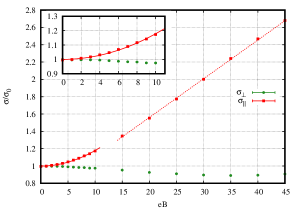
Figure 1: The ratios $\sigma_{\parallel,\perp}/\sigma_{0}$ as a function of the external magnetic field $eB$. The system is in the semimetal phase with the $\alpha_{eff}=0.32$. The $\sigma_{0}$ is the conductivity at $\alpha_{eff}=0.32$ at zero magnetic field. The external magnetic field $eB$ is shown in units $\frac{2\pi}{(a_{s}L_{s})^{2}}$. Red points correspond to conductivity parallel to the magnetic field $\sigma_{\parallel}$, green points give conductivity in the perpendicular direction $\sigma_{\perp}$ . Red lines correspond to quadratic and linear fit.

In order to get the theory for two Dirac fermions we numerically take square root of the fermion determinant. A detailed description of lattice action (8) and rooting procedure can be found in paper Braguta et al. (2017).

The fields $\theta_{i}$ describe the external magnetic field. Explicit expressions for the fields $\theta_{i}$ can be found in Al-Hashimi and Wiese (2009). It is important to notice here that due to the periodic boundary conditions on the $\theta_{i}$ magnetic field on the lattice is quantized

$$eB=\frac{2\pi N_{b}}{(a_{s}L_{s})^{2}},\qquad N_{b}\in\mathbb{Z}$$ (9)

The temperature on the lattice is given by the expression $T=1/(L_{t}a_{t})$. So, for the isotropic lattice $L_{s}=L_{t}$, $a_{s}=a_{t}$ the ratio $eB/T^{2}=2\pi N_{b}>1$, what does not allow to study the small magnetic field. In order to study the influence of the small magnetic field on the system we use anisotropic lattice with different lattice steps in temporal and spatial directions $a_{t}=\xi a_{s}$ with $\xi=1/4$.

To determine the electric conductivity we measured the Euclidean correlator $C_{i}(t)$ of the spatial components of electric current $j_{i}=\bar{\psi}\gamma_{i}\psi,~{}i=1,2,3$ (no summation over $i$ is assumed):

$$C_{i}(t)=\int d^{3}\bar{x}\langle j_{i}({\bar{x}},t)j_{i}(0)\rangle$$ (10)

In lattice simulations we used conserved current for staggered fermionsDeGrand and DeTar (2006):

$$j_{i}(x)=\frac{1}{4}(\bar{\Psi}_{x+i}\eta_{i}(x)U^{{\dagger}}_{i}(x)\Psi_{x}+\bar{\Psi}_{x}\eta_{i}(x)U_{i}(x)\Psi_{x+i})$$ (11)

Notice that in the continuum limit $a_{s}\to 0$ this current corresponds to usual electric current of 3D Dirac fermions $\bar{\psi}\gamma_{i}\psi$.

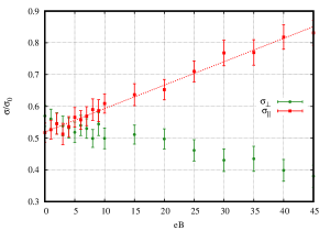
Figure 2: Same as in Fig. 1, but for $\alpha_{eff}=1.27$ where the system is in the onset of the insulator phase.

The correlator (10) is related to the conductivity $\sigma_{ii}(\omega)$ by means of Kubo relationBuividovich and Polikarpov (2012):

$$C_{i}(t)=\int\limits_{0}^{\infty}\frac{d\omega}{2\pi}K(\omega,t)\sigma_{ii}(\omega),$$ (12)

where $K(\omega,t)=\frac{2\omega\cosh(w(\frac{1}{2T}-t))}{\sinh(\frac{\omega}{2T})}$ is the standard thermal kernel. It should be noticed that the formula for the conductivity (5) was derived from real time equation. At the same time in lattice quantum Monte Carlo simulations we study the system in the thermodynamical equilibrium where there is no real time. In real time dynamics the electrical conductivity is related to the retarded Green function of the electromagnetic currents through Kubo relation. In turn the retarded Green function is related to the Euclidean correlation function of the electromagnetic currents (10). For this reason one can use the Euclidean correlation fuctions in order to study real time transport coefficients (see formula (12)). This approach is used in our paper.

In order to study the CME one needs the conductivity $\sigma_{ii}(\omega)$ at small frequencies. To calculate it one has to invert equation (12) what turns out to be very complicated problem. Typically there are several tens of points for $C_{i}(t)$ whereas one has to determine the continuous function $\sigma_{ii}(\omega)$.

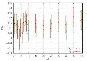
Figure 3: Same as in Fig. 1, but for $\alpha_{eff}=2.55$ where the system is deep in the insulator phase. In order to avoid superposition of data points for $\sigma_{\parallel}$ and $\sigma_{\perp}$ we applied a tiny shift along the $eB$ axis.

In this paper we are going to use midpoint calculation of the conductivityBuividovich and Polikarpov (2012):

$$\bar{\sigma}_{ii}=\int\limits_{0}^{\infty}\frac{d\omega}{2\pi}\frac{2\omega}{\sinh\frac{\omega}{2T}}\sigma_{ii}(\omega)/\int\limits_{0}^{\infty}\frac{d\omega}{2\pi}\frac{2\omega}{\sinh\frac{\omega}{2T}}=\frac{1}{\pi T^{2}}C_{i}\biggl{(}\frac{1}{2T}\biggr{)}$$ (13)

Physically the estimator $\bar{\sigma}_{ii}$ averages the conductivity over the interval $\sim\mbox{few}\times T$.

In the calculation we use the lattice with the size $L_{s}=L_{t}=20$, the asymmetry $\xi=a_{t}/a_{s}=1/4$ (one can expect that this value is close to the limit $\xi\to 0$Braguta et al. (2017)) and the fermion mass in lattice units $m=0.0025$. Lattice simulation are carried out for the effective coupling constant $\alpha_{eff}=2.55,1.27,0.32$. At $\alpha_{eff}^{c}=1.14$ there is transition from the semimetal to the insulator phase with dynamical breaking of the chiral symmetryBraguta et al. (2017). So the system with $\alpha_{eff}=0.32$ is in the semimetal phase. The $\alpha_{eff}=1.27$ corresponds to the insulator phase but close to the transition point $\alpha_{eff}^{c}$ (the onset of the insulator phase). The system with $\alpha_{eff}=2.55$ is deep in the insulator phase. For each value of the $\alpha_{eff}$ the simulations are conducted for a set of values of external magnetic field. For this set of parameters we calculated midpoint conductivity perpendicular $\sigma_{\perp}=\bar{\sigma}_{xx}$ and parallel $\sigma_{\parallel}=\bar{\sigma}_{zz}$ to the applied magnetic field.

In Fig. 1, 2, 3 we plot the ratios $\sigma_{\parallel,\perp}/\sigma_{0}$ as a function of the magnetic field $eB$ for different values of the $\alpha_{eff}$: $\alpha_{eff}=0.32$ (the semimetal phase, Fig. 1), $\alpha_{eff}=1.27$ (the onset of the insulator phase, Fig. 2) and $\alpha_{eff}=2.55$ (deep in the insulator phase, Fig. 3). The $\sigma_{0}$ is conductivity $\bar{\sigma}_{xx}$ at $\alpha_{eff}=0.32$ at zero magnetic field. Red points on these figures correspond to conductivity parallel to the magnetic field $\sigma_{\parallel}$, green points give conductivity in the perpendicular direction $\sigma_{\perp}$.

First let us consider Fig. 1 where the system is in the semimetal phase with $\alpha_{eff}=0.32$. It is clearly seen $\sigma_{\parallel}$ grows whereas $\sigma_{\perp}$ drops with the magnetic field. So we see positive magnetoresistance for the $\sigma_{\perp}$ and negative magnetoresistance for the $\sigma_{\parallel}$ what agrees with our expectation and the experiment Li et al. (2016a). Notice that there are two regimes of the dependence of the conductivity $\sigma_{\parallel}(B)$ on the magnetic field. For small values of magnetic field the $\sigma_{\parallel}(B)$ is quadratically rising function, while for larger values of magnetic field it is linearly rising function. This behaviour of the $\sigma_{\parallel}$ is in agreement with our expectation from formula (5). This brings us to the conclusion that we observe the CME in the lattice simulation of Dirac semimetals in the semimetal phase.

Further let us consider Fig. 2 with the $\alpha_{eff}=1.27$ where the system is in the onset of the insulator phase. From Fig. 2 it is seen that the $\sigma_{\parallel}(B)$ and $\sigma_{\perp}(B)$ behave similarly to the semimetal phase, but their absolute values are smaller and the CME is weaker.

Finally in Fig. 3 the results for the system deep in the insulator phase with $\alpha_{eff}=2.55$ are shown. It is seen that the conductivity is close to zero, it does not depend on the magnetic field and we do not observe the CME.

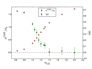
Figure 4: The left $y$-axis is the ratio of the CME conductivity $\sigma^{CME}$ for the magnetic field $eB(a_{s}L_{s})^{2}/(2\pi)=40$ to the $\sigma_{0}$ (green points) as a function of the effective coupling constant $\alpha_{eff}$. The right $y$-axis is the chiral condensate $\bar{\psi}\psi$ (red points) for the $eB(a_{s}L_{s})^{2}/(2\pi)=40$ as a function of the $\alpha_{eff}$.

In order to get more insight about how the CME is affected by the chiral symmetry breaking in Dirac semimetals we measured the CME conductivity $\sigma^{CME}$ and the chiral condensate $\bar{\psi}\psi$ for the magnetic field $eB(a_{s}L_{s})^{2}/(2\pi)=40$ for different values of the effective coupling constant $\alpha_{eff}$. In Fig. 4 we plot the ratio of the CME conductivity $\sigma^{CME}$ to the $\sigma_{0}$ (green points) as a function of the effective coupling constant $\alpha_{eff}$. On the same figure we also plot the chiral condensate $\bar{\psi}\psi$ (red points) as a function of the $\alpha_{eff}$.

To understand the physical meaning of Fig. 4 let us recall that the chiral condensate is sensitive to the dynamical chiral symmetry breaking/restoration transition. In the region $\alpha_{eff}<1$ the chiral condenstate is small and the chiral symmetry is not dynamically broken. In the region $\alpha_{eff}>1.4$ the chiral consensate is large and the chiral symmetry is dynamically broken. In the region $1<\alpha_{eff}<1.4$ we see rapid rise of the chiral condensate what implies that this is transition region between these two regimes. The critical coupling constant for this transition is $\alpha_{eff}^{c}\simeq 1.1$. Now let us consider the dependense of the CME conductivity $\sigma^{CME}$ on the $\alpha_{eff}$. It is seen from Fig. 4 that in the region $\alpha_{eff}<1$ the $\sigma^{CME}$ weakly depends on the $\alpha_{eff}$. However, for the $\alpha_{eff}>1$ we observe rapid decrease of the conductivity. Finally in the region $\alpha_{eff}>1.4$ the CME conductivity is zero within the uncertainty of the calculations. Notice that the region where the chiral condensate rises coincides with the region where the CME conductivity drops. This confirms that the CME conductivity is very sensitive to the chiral symmetry and dynamical breaking of the chiral symmetry in the system.

To summarize, the CME can be well seen in the semimetal phase where the chiral symmetry is not dynamically broken. It is also seen that the CME conductivity rapidly drops in the region where there is the transition from the phase with chiral symmetry to the phase where the chiral symmetry is dynamically broken. Finally in the region where the system is deep in the insulator phase with dynamically broken chiral symmetry the CME conductivity is zero within the uncertainty of the calculation. This behaviour of the conductivity can be understood as follows. Generation of the CME current is connected with the Schwinger pair production on the lowest Landau levelKharzeev et al. (2013b). In the insulator phase due to chiral symmetry breaking there is dynamical generation of the fermion mass whereas in the semimetal phase there is no dynamical fermion mass. The deeper to the insulator phase the larger the dynamical fermion mass. Note also that the larger the fermion mass the larger suppression of the Schwinger pair production. For this reason one can expect that the CME is suppressed in the onset of the insulator phase as compared to the semimetal phase. It is also reasonable to assume that there is no CME deep to the insulator phase since the dynamical fermion mass is large and the Schwinger pair production at the lowest Landau level is considerably suppressed.

In conclusion, in this paper the Chiral Magnetic Effect in Dirac semimetals was studied by means of lattice Monte Carlo simulation. The simulations were carried out in three regimes: semimetal phase, onset of the insulator phase and deep in the insulator phase. We observe manifestation of the CME current in the semimetal phase, weaker manifestation of the CME in the onset of the insulator phase. We do not observe the CME in the insulator phase.

In order to get more insight about how the CME is affected by the chiral symmetry breaking we measured the CME conductivity and the chiral condensate at large magnetic field as a function of the effective coupling constant $\alpha_{eff}$. We found that the large the chiral condensate the smaller the CME conductivity. Thus we confirmed that the CME conductivity is very sensitive to the chiral symmetry and dynamical breaking of the chiral symmetry in the system.