Computation of three-dimensional three-phase flow of carbon dioxide using a high-order WENO scheme

Abstract

We have developed a high-order numerical method for the 3D simulation of viscous and inviscid multiphase flow described by a homogeneous equilibrium model and a general equation of state. Here we focus on single-phase, two-phase (gas-liquid or gas-solid) and three-phase (gas-liquid-solid) flow of $\text{CO}_{\text{2}}$ whose thermodynamic properties are calculated using the Span–Wagner reference equation of state. The governing equations are spatially discretized on a uniform Cartesian grid using the finite-volume method with a fifth-order weighted essentially non-oscillatory (WENO) scheme and the robust first-order centred (FORCE) flux. The solution is integrated in time using a third-order strong-stability-preserving Runge–Kutta method. We demonstrate close to fifth-order convergence for advection-diffusion and for smooth single- and two-phase flows. Quantitative agreement with experimental data is obtained for a direct numerical simulation of an air jet flowing from a rectangular nozzle. Quantitative agreement is also obtained for the shape and dimensions of the barrel shock in two highly underexpanded $\text{CO}_{\text{2}}$ jets.

1 Introduction

The deployment of $\text{CO}_{\text{2}}$ capture and storage (CCS) is regarded as a key strategy to mitigate global warming [1]. To design and operate CCS systems in a safe and cost-effective way, accurate data and models are needed [2]. This includes models and methods to simulate the near field of a $\text{CO}_{\text{2}}$ jet resulting from the decompression of equipment containing high-pressure $\text{CO}_{\text{2}}$. The data from these near-field simulations are e.g. used as input for less resolved simulations of the dispersion of $\text{CO}_{\text{2}}$ in the terrain [3, 4, 5].

This type of scenario puts some requirements on the models and numerical methods to be used. Depressurization of $\text{CO}_{\text{2}}$ from supercritical pressures typically involves complex three-phase (gas-liquid-solid) flow. Describing this kind of flow necessitates a multiphase flow model and an equation of state (EOS) that is accurate and capable of capturing the three-phase behaviour [6, 7]. For high vessel pressures, the $\text{CO}_{\text{2}}$ jet resulting from a leak will form a shock, which the numerical method must be able to capture. In addition, we would like the numerical method to maintain discrete conservation of mass, momentum and energy and, due to computational efficiency, to be of high order in smooth regions of the computational domain, without producing spurious oscillations in the solution near discontinuities.

Wareing et al. [7, 8] and Woolley et al. [9] studied $\text{CO}_{\text{2}}$ jets using a Reynolds-averaged Navier–Stokes model. The flow model was combined with a composite EOS [7] to describe three-phase $\text{CO}_{\text{2}}$ flow. The flow model was solved using a conservative, shock-capturing second-order scheme, as described by Falle [10].

However, advances have been made in constructing and implementing finite-volume, shock capturing and conservative numerical methods of higher order. Titarev and Toro [11] presented a procedure relying on weighted essentially non-oscillatory (WENO) interpolation [12] and achieved fifth-order convergence for their smooth and inviscid two-dimensional isentropic vortex problem. Their scheme was extended to include interpolation of velocity derivatives and computation of viscous transport of momentum and dissipation of kinetic energy by Coralic and Colonius [13]. Such a numerical scheme is suitable for execution on parallel computers by domain decomposition [14].

In research on numerical methods for compressible multiphase flow, the ideal-gas and stiffened-gas EOS [15, 16] are commonly employed, due to their simplicity and relatively large number of applications. This is true both for 1D [17, 18, 19] and 3D models [e.g. 13]. The stiffened-gas EOS can be regarded as a linearization about a reference state. In many cases, however, it is necessary to consider more adapted EOSs in order to achieve the necessary accuracy. This often entails a significantly higher computational complexity. As an example, Dumbser et al. [20] presented an unstructured WENO scheme employing a real EOS for water.

For CCS applications, it is often necessary to describe a large thermodynamic property space, involving multiple phases, for instance for the depressurization from a transport pipeline operated at a supercritical pressure around $100\text{\,}\mathrm{bar}\text{/}$ down to atmospheric conditions. In these cases, an accurate EOS is required [6], such as the one by Span and Wagner [21] (SW). Therefore, in order to perform high-fidelity near-field studies of $\text{CO}_{\text{2}}$ jets, we need to combine a high-order numerical scheme with a general EOS.

This combination would also benefit the development of predictive fluid-structure models aiding in the design of $\text{CO}_{\text{2}}$-transport pipelines against running fractures [22, 23]. For practical and computational reasons, the $\text{CO}_{\text{2}}$ flow is commonly described using a 1D model, which implies a simplified description of the pressure forces on the opening pipe flanks [22]. A full 3D description of the flow might provide more accurate predictions.

In the present work we want to study complex $\text{CO}_{\text{2}}$ flows which may be single phase, two-phase (gas-liquid or gas-solid) or three-phase (gas-liquid-solid). In doing so, we extend the high-order scheme of Titarev and Toro [11] and Coralic and Colonius [13], applying it to the homogeneous equilibrium multiphase flow model and a formulation allowing the use of a general EOS. Since the applications we are interested in typically involve sharp temperature gradients, we include heat conduction in our model and in the numerical treatment of diffusive fluxes, as well as a temperature-dependent viscosity.

We validate the implementation of the model and numerical methods through several test cases, including a turbulent air jet from a rectangular nozzle. We also demonstrate that the numerical methods exhibit high-order convergence when dealing with diffusive fluxes and two-phase flows. Finally, we perform detailed simulations of $\text{CO}_{\text{2}}$ jets, employing the SW EOS.

The rest of this paper is organized as follows. Section 2 reviews the governing equations, while the treatment of inflow and open boundary conditions is briefly described in Section 3. Section 4 deals with the numerical methods. Section 5 demonstrates the accuracy and robustness of the scheme, including the direct numerical simulation of an air jet, while Section 6 discusses the simulation of a $\text{CO}_{\text{2}}$ jet. Section 7 concludes the study.

2 Models

2.1 Fluid dynamics

We consider a three-dimensional flow of a fluid that may consist of multiple phases. The different phases are assumed to be in local equilibrium and to move with the same velocity. The flow may then be described by a homogenous equilibrium model (HEM), which can be formulated as a system of balance equations,

$$\partial_{t}\boldsymbol{Q}+\partial_{x}\boldsymbol{F}+\partial_{y}\boldsymbol{G}+\partial_{z}\boldsymbol{H}=\boldsymbol{S}(\boldsymbol{Q}).$$ (1)

Here $\boldsymbol{F}$, $\boldsymbol{G}$ and $\boldsymbol{H}$ are the fluxes in the $x$-, $y$- and $z$-direction, respectively, and $\boldsymbol{S}(\boldsymbol{Q})$ is the vector of source terms. The vector $\boldsymbol{Q}$ contains the state variables,

$$\boldsymbol{Q}=\left[\rho,\rho u_{x},\rho u_{y},\rho u_{z},E\right]^{\text{T}},$$ (2)

where $\rho$ is the fluid density, $u_{x}$, $u_{y}$ and $u_{z}$ are the flow velocities and $E$ is the total energy density. Thus the system (1) describes conservation of mass and balance of momentum and energy of the fluid. The total energy is

$$E=\rho e+\frac{1}{2}\rho\left(u_{x}^{2}+u_{y}^{2}+u_{z}^{2}\right),$$ (3)

where $e$ is the specific internal energy of the fluid. The total energy is thus the sum of internal and kinetic energy.

The fluxes are

$$\boldsymbol{F}=\begin{bmatrix}\rho u_{x}\\ \rho u_{x}^{2}+p-\sigma_{xx}\\ \rho u_{y}u_{x}-\sigma_{xy}\\ \rho u_{z}u_{x}-\sigma_{xz}\\ (E+p)u_{x}-u_{i}\sigma_{xi}-\kappa\partial_{x}T\end{bmatrix},$$ (4)

$$\boldsymbol{G}=\begin{bmatrix}\rho u_{y}\\ \rho u_{x}u_{y}-\sigma_{yx}\\ \rho u_{y}^{2}+p-\sigma_{yy}\\ \rho u_{z}u_{y}-\sigma_{yz}\\ (E+p)u_{y}-u_{i}\sigma_{yi}-\kappa\partial_{y}T\end{bmatrix},$$ (5)

and

$$\boldsymbol{H}=\begin{bmatrix}\rho u_{z}\\ \rho u_{x}u_{z}-\sigma_{zx}\\ \rho u_{y}u_{z}-\sigma_{zy}\\ \rho u_{z}^{2}+p-\sigma_{zz}\\ (E+p)u_{z}-u_{i}\sigma_{zi}-\kappa\partial_{z}T\end{bmatrix}.$$ (6)

Herein, $p$ is the fluid pressure, $T$ is the temperature, $\kappa$ is the thermal conductivity and $\sigma_{ij}$ is the viscous stress tensor. With these fluxes, and no source terms, (1) corresponds to the Euler equations with added diffusive fluxes for viscous transport of momentum and conductive transport of heat.

We assume zero bulk viscosity, in which case the viscous stress tensor is given by the velocity derivatives and the dynamic viscosity $\eta$ as [24]

$$\sigma_{ij}=\eta\left(\partial_{i}u_{j}+\partial_{j}u_{i}-\frac{2}{3}\delta_{ij}\partial_{k}u_{k}\right).$$ (7)

2.2 Thermophysical properties

In order to close the system (1), we must employ a thermodynamic equation of state (EOS). We assume local thermodynamic phase equilibrium and consider only pure components. In this paper, we make use of the ideal gas EOS (IG), the Peng–Robinson [25] EOS (PR) and the multi-parameter Span–Wagner [21] reference EOS (SW) for $\text{CO}_{\text{2}}$. Both PR and SW describe gas-liquid systems. By coupling SW to an additional model for the solid $\text{CO}_{\text{2}}$ phase, it can be extended to systems including a solid phase and be used to describe solid formation, as described in Hammer et al. [6].

The thermal conductivity $\kappa$ is assumed constant throughout this work. The dynamic viscosity $\eta$, however, has a strong temperature dependence and cannot always be assumed constant. Therefore, we use the TRAPP extended corresponding state model due to Ely and Hanley [26] for the dynamic viscosity in cases with large temperature variations.

3 Boundary conditions

3.1 Nozzle inflow

For the $\text{CO}_{\text{2}}$ jet to be studied, we model inflow through a nozzle located at the domain boundary. Boundary conditions in the nozzle region are set by the isentropic steady-state Bernoulli equations,

$$\mathop{\mathrm{\mathstrut d}}\nolimits\!h+u\mathop{\mathrm{\mathstrut d}}\nolimits\!u =0,$$ (8)

$$\mathop{\mathrm{\mathstrut d}}\nolimits\!s =0,$$ (9)

for the specific enthalpy $h$, specific entropy $s$ and velocity $u$ of the fluid. Integrating these to the boundary from some known rest state behind the nozzle, specified e.g. by $T_{\infty}$ and $p_{\infty}$, we get

$$s_{\infty} =s_{\text{b}},$$ (10)

$$h_{\infty} =h(s_{\text{b}},p_{\text{b}})+\frac{1}{2}u_{\text{b}}^{2},$$ (11)

where the boundary values have a subscript b. By setting $u_{\text{b}}$ equal to the speed of sound and solving the integrated Bernoulli equations for $p_{\text{b}}$, we obtain the choke pressure at the nozzle. This procedure thus gives the pressure, entropy and flow velocity at the boundary and the boundary condition is completely specified.

3.2 Non-reflecting boundaries

Many practical flows of interest are located in physical domains that are unbounded in one or more spatial directions and require the specification of an artificial boundary in order to make the computational domain finite. The artificial boundary represents a connection between the computational domain and the surrounding far field. Care must be taken in the definition of this open boundary. Under-specification or over-specification of physical boundary conditions would lead to an ill-posed problem and are a classical cause of numerical instability. In fluid flows, information about the flow conditions is transmitted across the open boundaries by physical waves. These open boundaries should allow waves (especially pressure waves or acoustic waves) to travel freely in and out of the computational domain. However, the knowledge about the exterior can often be unsure or absent and additional modelling or qualified guesses about these flow conditions may be necessary. In particular, the amplitudes of the outgoing waves may be used as a starting point for the modelling of the incoming ones. This approach, named Navier–Stokes Characteristic Boundary Conditions (NSCBC), is utilized in the present work to specify the open boundaries of the computational domain, as described in the landmark paper by Poinsot and Lele [27] and later refined by Sutherland and Kennedy [28] for the general context of single-phase, multi-component and reactive flows.

4 Numerical methods

The fluid-dynamical model is integrated in time using the finite-volume method on a uniform Cartesian grid. This method transforms the coupled system of PDEs (1) into a system of coupled ODEs that can be integrated in time with an appropriate Runge–Kutta method.

4.1 Spatial discretization

The semi-discrete form of the PDE system (1) is obtained by integrating it over the volume of a cell $i,j,k$ and applying the divergence theorem,

$$\frac{\mathop{\mathrm{\mathstrut d}}\nolimits\!missing}{\mathop{\mathrm{\mathstrut d}}\nolimits\!{t}}\boldsymbol{Q}_{i,j,k}=\ \frac{1}{\Delta x}\left(\boldsymbol{F}_{i-1/2,j,k}-\boldsymbol{F}_{i+1/2,j,k}\right)+\frac{1}{\Delta y}\left(\boldsymbol{G}_{i,j-1/2,k}-\boldsymbol{G}_{i,j+1/2,k}\right)+\frac{1}{\Delta z}\left(\boldsymbol{H}_{i,j,k-1/2}-\boldsymbol{H}_{i,j,k+1/2}\right).$$ (12)

Herein, we have defined the volume-averaged state variables for the cell $i,j,k$,

$$\boldsymbol{Q}_{i,j,k} \equiv\frac{1}{\Delta x\Delta y\Delta z}\int_{x_{i-1/2}}^{x_{i+1/2}}\int_{y_{j-1/2}}^{y_{j+1/2}}\int_{z_{k-1/2}}^{z_{k+1/2}}\boldsymbol{Q}\left(x,y,z,t\right)\ \mathop{\mathrm{\mathstrut d}}\nolimits\!x\mathop{\mathrm{\mathstrut d}}\nolimits\!y\mathop{\mathrm{\mathstrut d}}\nolimits\!z,$$ (13)

and the area-averaged fluxes over the cell edges,

$$\boldsymbol{F}_{i-1/2,j,k} \equiv\frac{1}{\Delta y\Delta z}\int_{y_{j-1/2}}^{y_{j+1/2}}\int_{z_{k-1/2}}^{z_{k+1/2}}\boldsymbol{F}\left(x_{i-1/2},y,z,t\right)\ \mathop{\mathrm{\mathstrut d}}\nolimits\!y\mathop{\mathrm{\mathstrut d}}\nolimits\!z,$$ (14)

$$\boldsymbol{G}_{i,j-1/2,k} \equiv\frac{1}{\Delta x\Delta z}\int_{x_{i-1/2}}^{x_{i+1/2}}\int_{z_{k-1/2}}^{z_{k+1/2}}\boldsymbol{G}\left(x,y_{j-1/2},z,t\right)\ \mathop{\mathrm{\mathstrut d}}\nolimits\!x\mathop{\mathrm{\mathstrut d}}\nolimits\!z,$$ (15)

$$\boldsymbol{H}_{i,j,k-1/2} \equiv\frac{1}{\Delta x\Delta y}\int_{x_{i-1/2}}^{x_{i+1/2}}\int_{y_{j-1/2}}^{y_{j+1/2}}\boldsymbol{H}\left(x,y,z_{k-1/2},t\right)\ \mathop{\mathrm{\mathstrut d}}\nolimits\!x\mathop{\mathrm{\mathstrut d}}\nolimits\!y.$$ (16)

Approximating the flux integrals (14)-(16) using one quadrature point per cell edge, one may derive numerical schemes that are at most second-order. If one instead evaluates the flux integrals using multiple quadrature points on each cell edge, numerical methods of higher order can be constructed. The evaluation of the flux integrals is then done by first computing the numerical flux at each quadrature point, and then taking some linear combination of the computed fluxes. This procedure requires reconstruction of the fluid state and derivatives of velocity and temperature to both sides of the cell edges at each quadrature point. It also requires high-order numerical volume integration when calculating the volume-averaged primitive variables $\boldsymbol{V}_{i,j,k}$ from the state variables $\boldsymbol{Q}$, as noted by Coralic and Colonius [13]. That is, the integral

$$\boldsymbol{V}_{i,j,k} \equiv\frac{1}{\Delta x\Delta y\Delta z}\int_{x_{i-1/2}}^{x_{i+1/2}}\int_{y_{j-1/2}}^{y_{j+1/2}}\int_{z_{k-1/2}}^{z_{k+1/2}}\boldsymbol{V}\left(\boldsymbol{Q}\left(x,y,z,t\right)\right)\ \mathop{\mathrm{\mathstrut d}}\nolimits\!x\mathop{\mathrm{\mathstrut d}}\nolimits\!y\mathop{\mathrm{\mathstrut d}}\nolimits\!z,$$ (17)

must be approximated numerically using multiple quadrature points per cell volume and thus the state variables must be reconstructed to these quadrature points.

Titarev and Toro [11] presented a procedure as outlined above using WENO interpolation for reconstruction of the fluid states. This was extended to include reconstruction of derivatives and computation of diffusive fluxes by Coralic and Colonius [13]. We will rely on their methods in this work and the reader is referred to their works for a more thorough exposition. We shall here employ a fifth-order WENO scheme for reconstruction of fluid states and use fourth-order Gaussian quadrature rules, two quadrature points for each cell edge integral and four quadrature points for each cell volume integral, in all 2D simulations. In 3D, we shall use four quadrature points for each cell edge integral and eight quadratures point for each cell volume integral. As basic advective numerical flux, we employ the robust first-order centred (FORCE) scheme [29]. Regarding the calculation of the WENO weights, we employ the relations presented in [11].

4.1.1 Reconstructed variables

In order for the fluid states at the quadrature points to be consistent with the EOS, one must choose a set of five variables, interpolate these to the quadrature points and then use the interpolated values, the EOS and the thermophysical property models to compute the remaining variables needed to compute the fluxes. As noted by e.g. Coralic and Colonius [13], the fluid state may be reconstructed using many different sets of variables, i.e. the choice of reconstruction variables is not unique. To avoid spurious oscillations, however, it will often be necessary to reconstruct in another set of variables than the state variables $\boldsymbol{Q}$ [30, Sec. 14.4.3]

Hammer et al. [6] performed reconstruction in flow velocity, density and internal energy when performing 1D simulations with second-order MUSCL reconstruction and the Span–Wagner reference EOS for $\text{CO}_{\text{2}}$. For simulations with high-order WENO reconstruction and the ideal gas or stiffened-gas EOS, Titarev and Toro [11] and Coralic and Colonius [13] performed reconstruction in the local characteristic variables. Coralic and Colonius [13] obtained the local characteristic variables by multiplying the vector of primitive variables with a locally frozen transformation matrix. We will follow their procedure when using the ideal-gas EOS. However, for more advanced EOSs, we use a more general procedure which is described in A.

4.2 Temporal integration

For time integration, we use the three-step third-order strong-stability-preserving Runge–Kutta (RK) method [see e.g. 31]. Our time steps are limited by a Courant–Friedrichs–Lewy (CFL) criterion for all cases. This is done in a similar way as in [11]. For cases with viscosity and thermal conductivity, one must in addition consider the time step restriction imposed by the diffusive fluxes [13]. Given a set of fluid parameters, the latter restriction will be limiting for the time step length if fine enough grids are used. In practice, however, we found that the CFL criterion was sufficient to ensure stability for the grids and fluids considered in this study.

4.3 Phase equilibrium

When the balance equations (1) are advanced in time, the mass of each component, and the momentum and total energy of the mixture are updated in every control volume. This allows the determination of the specific volume ${v}$ and internal energy ${e}$. For given ${e}$ and ${v}$, the equilibrium phase distribution and the intensive variables temperature $T$ and pressure $p$ must be determined. This calculation is called a flash, or more specifically an ${e}{v}$-flash. Mathematically, the ${e}{v}$-flash represents a global maximization of entropy in the temperature-pressure-phase-fraction space, subject to constraints on mass and internal energy. A challenging part of this calculation is to determine which phases are present. Under the assumption of full equilibrium (mechanical, thermal and chemical), the phases present must have the same pressure, temperature and chemical potential. For our numerical methods, we guess which phases are present and then solve to meet the constrains. During this iterative procedure, all phases present are in full equilibrium. When the constraints are satisfied for the trial set of phases, it must be determined if the solution is a local or a global solution by introducing or removing phases. The phase distribution maximizing the entropy is the ${e}{v}$-flash solution.

At different steps in the model integration, it becomes necessary to solve different flash problems. These are still global optimization problems, but they have constraints other than mass and internal energy. Depending on what information is available at a given step, we solve one of the following problems to obtain the equilibrium state.

• Equilibrium calculation with specified internal energy ${e}_{\text{spec}}$ and specific volume ${v}_{\text{spec}}$ (${e}{v}$-flash)

• Equilibrium calculation with specified entropy ${s}_{\text{spec}}$ and specific volume ${v}_{\text{spec}}$ (${s}{v}$-flash)

• Equilibrium calculation with specified entropy ${s}_{\text{spec}}$ and pressure $p_{\text{spec}}$ ($p{s}$-flash)

When performing reconstruction in internal energy, density and velocity, we have a known internal energy $e_{\text{spec}}$ and specific volume ${v}_{\text{spec}}$. To determine the temperature, pressure and phase distribution, an ${e}{v}$-flash must be solved.

To set boundary-condition states from the nozzle inflow model (see Section 3.1), we must calculate the equilibrium state with specified pressure $p_{\text{spec}}$ and entropy $s_{\text{spec}}$. To determine the temperature and the phase fractions, the $p{s}$-flash must be solved.

Giljarhus et al. [32] considered these equilibrium problems for single-phase gas and liquid, and two-phase gas-liquid. The extension of the solution procedures to account for dry-ice along the sublimation line is described thoroughly by Hammer et al. [6], for both the ${e}{v}$-flash and the $p{s}$-flash. The ${s}{v}$-flash has not been considered earlier and will be treated in more detail below. We do not rely on tabulated values in the numerical procedures, but solve the EOS directly.

4.3.1 The ${s}{v}$-flash

When computing the equilibrium fluid states from the set of variables $\boldsymbol{R}$ available when reconstructing in the local characteristic variables (see A), we must perform an equilibrium calculation with specified entropy $s_{\text{spec}}$ and specific volume ${v}_{\text{spec}}$. The whole procedure is analogous to that with specified $e_{\text{spec}}$ and $v_{\text{spec}}$.

In principle, the EOSs we consider here can be expressed in terms of the specific Helmholtz free energy as a function of temperature and density, $a(T,\rho)$. All other thermodynamic properties can be written in terms of $a$ and its derivatives. Thus, in the gas-liquid case, solving the equation set

$$\boldsymbol{\varphi}\left(\rho_{\text{g}},\rho_{\ell}\right)=\begin{bmatrix}\mu\left(T,\rho_{\text{g}}\right)-\mu\left(T,\rho_{\ell}\right)\\ p\left(T,\rho_{\text{g}}\right)-p\left(T,\rho_{\ell}\right)\end{bmatrix}=\boldsymbol{0},$$ (18)

yields $\rho_{\text{g}}^{\text{sat}}$ and $\rho_{\ell}^{\text{sat}}$ for a given $T$. $\mu$ denotes the chemical potential. Here and in the following, $\boldsymbol{\varphi}$ is a general set of thermodynamic relations which form the left-hand side of an equation set to be solved. With the phase densities as functions of temperature, the entropy and specific volume constraints can be solved for in an outer loop,

$$\boldsymbol{\varphi}\left(T,\beta_{\text{g}}\right)=\begin{bmatrix}{v}\left(T,\beta_{\text{g}}\right)-{v}_{\text{spec}}\\ {s}\left(T,\beta_{\text{g}}\right)-{s}_{\text{spec}}\end{bmatrix}=\boldsymbol{0},$$ (19)

to get the equilibrium temperature and the gas mass fraction $\beta_{\text{g}}$. It is also possible to solve (18) and (19) simultaneously, but solving them in an nested-loop approach improves the robustness. The gas-solid equilibrium case is solved in a similar manner as the gas-liquid case.

In the case where the equilibrium state is single-phase, the EOS provides the relation $p=p\left(T,1/{v}_{\text{spec}}\right)$ and we solve

$$\varphi\left(T\right)=\left({s}\left(T\right)-{s}_{\text{spec}}\right)=0,$$ (20)

to obtain the equilibrium temperature.

In the gas-liquid-solid equilibrium case, i.e. the triple point, we solve

$$\boldsymbol{\varphi}\left(\beta_{\text{g}},\beta_{\ell},\beta_{\text{s}}\right)=\begin{bmatrix}{v}^{\text{tr}}_{\text{g}}\beta_{\text{g}}+{v}^{\text{tr}}_{\ell}\beta_{\ell}+{v}^{\text{tr}}_{\text{s}}\beta_{\text{s}}-{v}_{\text{spec}}\\ {s}^{\text{tr}}_{\text{g}}\beta_{\text{g}}+{s}^{\text{tr}}_{\ell}\beta_{\ell}+{s}^{\text{tr}}_{\text{s}}\beta_{\text{s}}-{s}_{\text{spec}}\\ \beta_{\text{g}}+\beta_{\ell}+\beta_{\text{s}}-1\end{bmatrix}=\boldsymbol{0},$$ (21)

to obtain the phase mass fractions $\beta_{\text{g}}$, $\beta_{\ell}$ and $\beta_{\text{s}}$. Properties with superscript tr are evaluated for the triple-point pressure and temperature.

4.4 Speed of sound

The speed of sound $c$ for a single-phase fluid is computed as

$$c=\sqrt{\left(\frac{\partial p}{\partial\rho}\right)_{s}}.$$ (22)

For a gas-liquid mixture in equilibrium, the mixture speed of sound can be calculated from the combined ${s}{v}$-flash condition (19), and the modified saturation line condition (18), resulting in the following system of equations:

$$\boldsymbol{\varphi}\left(T,p,\beta_{\text{g}},\rho_{\text{g}},\rho_{\ell}\right)=\begin{bmatrix}\mu\left(T,\rho_{\text{g}}\right)-\mu\left(T,\rho_{\ell}\right)\\ p-p\left(T,\rho_{\text{g}}\right)\\ p-p\left(T,\rho_{\ell}\right)\\ {v}\left(T,\beta_{\text{g}},\rho_{\text{g}},\rho_{\ell}\right)-{v}_{\text{spec}}\\ {s}\left(T,\beta_{\text{g}},\rho_{\text{g}},\rho_{\ell}\right)-{s}_{\text{spec}}\end{bmatrix}=\boldsymbol{0}.$$ (23)

The solution $\boldsymbol{\chi}=\left[T,p,\beta_{\text{g}},\rho_{\text{g}},\rho_{\ell}\right]^{\text{T}}$ to (23) gives a relation for ${v}_{\text{spec}}$ and ${s}_{\text{spec}}$:

$$\boldsymbol{\varphi}\left(\ \boldsymbol{\chi}\left({v}_{\text{spec}},{s}_{\text{spec}}\right),{v}_{\text{spec}},{s}_{\text{spec}}\right)=\boldsymbol{0}.$$ (24)

Differentiating with respect to ${v}_{\text{spec}}$, we obtain

$$\partial_{\boldsymbol{\chi}}\boldsymbol{\varphi}\ \partial_{{v}_{\text{spec}}}\boldsymbol{\chi}+\partial_{{v}_{\text{spec}}}\boldsymbol{\varphi}=\boldsymbol{0},$$ (25)

whose solution $\partial_{{v}_{\text{spec}}}\boldsymbol{\chi}$ gives an isentropic $\partial_{{v}_{\text{spec}}}p$, that can readily be used to calculate the mixture speed of sound. A similar approach is used to calculate the speed of sound for a gas-solid mixture. For coexistence of solid, gas and liquid, the equilibrium model predicts that the speed of sound is zero, since the density can change isentropically without a change in pressure [33, Sec. 2.8.1]. Hence, at the triple point, the HEM loses hyperbolicity. Although this behaviour is believed to be unphysical, it has not caused practical problems in the present simulations.

4.5 Parallelization

It is a computationally intensive task to solve any CFD problem in three dimensions. Advanced thermodynamic models, like the EOSs used here, add even more to the computational load. It is therefore necessary to run simulations in parallel on high-performance computing (HPC) machines.

Since we here use explicit time integration methods, the parallelization becomes relatively straightforward. In particular, we apply a blockwise domain decomposition [34] to the spatial domain, and the spatial discretization is applied to the subdomains which are distributed over the nodes of the HPC cluster using MPI for communication. Due to the width of the WENO stencils, we require three ghost cells both on the physical domain boundaries and on the internal boundaries of each subdomain. The values in the ghost cells are synchronized as necessary, e.g. before each substep in the temporal discretization.

The implementation of the domain decomposition is based on PETSc [14, 35]. In particular, we follow the minimally-intrusive parallelization strategy of Ervik et al. [36], where awareness of the decomposed nature of the domain is hidden from the majority of the code.

5 Validation

5.1 Advection-diffusion

To demonstrate the high-order convergence of the numerical methods for diffusive fluxes, we first consider a smooth problem with the 2D constant-coefficient advection-diffusion equation,

$$\partial_{t}q+u_{x}\partial_{x}q+u_{y}\partial_{y}q=D\left(\partial_{x}\partial_{x}q+\partial_{y}\partial_{y}q\right).$$ (26)

Here $q$ is some quantity subject to advective and diffusive transport, $u_{x}$ and $u_{y}$ are the advection velocities and $D$ is the diffusion coefficient. If we take the entire $x$-$y$ plane as our domain, an analytical solution to this equation is the Gaussian pulse,

$$q\left(x,y,t\right)=\frac{1}{2\pi\sigma^{2}(t)}\exp\left(-\frac{(x-u_{x}t-x_{0})^{2}}{2\sigma^{2}(t)}-\frac{(y-u_{y}t-y_{0})^{2}}{2\sigma^{2}(t)}\right).$$ (27)

Herein, $x_{0}$ and $y_{0}$ define the initial position of the Gaussian pulse and the spread of the pulse $\sigma^{2}(t)$ is a function of time $t$ and initial the spread $\sigma^{2}_{0}$ at $t=$0\text{\,}\mathrm{s}\text{/}$$,

$$\sigma^{2}(t)=2Dt+\sigma^{2}_{0}.$$ (28)

We consider the specific problem where $x_{0}=y_{0}=$3\text{/}8\text{\,}\mathrm{m}\text{/}$$, $\sigma_{0}=$1\text{/}16\text{\,}\mathrm{m}\text{/}$$, $u_{x}=u_{y}=$1\text{\,}\mathrm{m}\text{/}\mathrm{s}$$, and $D=$5\text{\times}{10}^{-3}\text{\,}{\mathrm{m}}^{2}\text{/}\mathrm{s}$$. We solve the problem inside a periodic domain $[0,1]\times[0,1]\,$\mathrm{m}\text{/}$$ and note that, with the specified parameters, the value of the solution at the domain boundaries will be much smaller than any numerical errors. The initial condition follows from (27) evaluated at $t=$0\text{\,}\mathrm{s}\text{/}$$.

The governing equation (26) is integrated to $t=$0.25\text{\,}\mathrm{s}\text{/}$$. To eliminate the effect of the RK method on the convergence order, we use a constant time step of ${10}^{-3}\text{\,}\mathrm{s}\text{/}$ for all grid sizes. This corresponds to a CFL number of 0.2 on the $200\times 200$ grid.

The analytical and numerical results at $t=$0.25\text{\,}\mathrm{s}\text{/}$$ are plotted in Figure 1. It is evident that the numerical solutions converge rapidly to the analytical solution when the grid is refined. The errors and the estimated convergence orders are presented in Table 1. The errors computed with the $L_{1}$-norm are normalized with respect to the number of grid cells. These results show fifth-order accuracy of the numerical method, also when treating both diffusive and advective fluxes. The convergence order is better than what we should expect, since we use a fourth-order accurate quadrature rule in integrating the fluxes.

The results presented in this section extend the results shown by Coralic and Colonius [13]. In their paper, convergence orders are only calculated, and shown to be of fifth-order, for the isentropic vortex case in the absence of any diffusive fluxes. By applying the numerical schemes to the advection-diffusion equation, we have demonstrated fifth-order convergence also when diffusive fluxes are included.

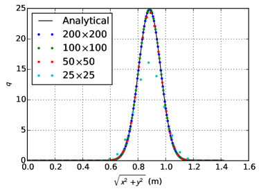
Figure 1: Comparison of the analytical solution and numerical results for the advection-diffusion problem. Values along the line $x=y$ are plotted.

Table 1: Errors and estimated convergence orders in the 2D advection-diffusion case.

Grid	$L_{1}$-error	$L_{1}$-order	$L_{\infty}$-error	$L_{\infty}$-order
$25\times 25$	$3.208\text{\times}{10}^{-01}\text{\,}\text{/}$	-	$8.637\text{\times}{10}^{00}\text{\,}\text{/}$	-
$50\times 50$	$1.112\text{\times}{10}^{-02}\text{\,}\text{/}$	$4.85\text{\,}\text{/}$	$4.536\text{\times}{10}^{-01}\text{\,}\text{/}$	$4.25\text{\,}\text{/}$
$100\times 100$	$2.543\text{\times}{10}^{-04}\text{\,}\text{/}$	$5.45\text{\,}\text{/}$	$1.060\text{\times}{10}^{-02}\text{\,}\text{/}$	$5.42\text{\,}\text{/}$
$200\times 200$	$8.953\text{\times}{10}^{-06}\text{\,}\text{/}$	$4.83\text{\,}\text{/}$	$3.674\text{\times}{10}^{-04}\text{\,}\text{/}$	$4.85\text{\,}\text{/}$

5.2 Isentropic vortex

To validate the convergence order of the numerical schemes when applied to the fluid model with a realistic EOS, we next consider a smooth, inviscid test problem. In particular, we consider a generalization of the isentropic vortex where the initial condition of the problem can be found for a general EOS. The isentropic vortex with ideal gas was studied by Balsara and Shu [37], by Titarev and Toro [11] and by Coralic and Colonius [13] to demonstrate the convergence order of their numerical schemes. In the following simulations, we first use the EOS of Peng and Robinson [25] for pure $\text{CO}_{\text{2}}$. Next, we consider the Span and Wagner [21] EOS.

To define the initial condition, we demand a uniform entropy $s$ and prescribe a rotating velocity field,

$$u_{x} =u_{x,\infty}-\frac{\epsilon y}{2\pi r_{0}}\exp\left(\frac{1-(r/r_{0})^{2}}{2}\right),$$ (29)

$$u_{y} =u_{y,\infty}+\frac{\epsilon x}{2\pi r_{0}}\exp\left(\frac{1-(r/r_{0})^{2}}{2}\right).$$ (30)

Herein $u_{x,\infty}$ and $u_{y,\infty}$ are constant background velocities, $\epsilon$ is the vortex strength and $r_{0}$ is the vortex radius. We let $u_{x,\infty}=u_{y,\infty}=$0\text{\,}\mathrm{m}\text{/}\mathrm{s}$$, $\epsilon=$1000\text{\,}\mathrm{m}\text{/}\mathrm{s}$$ and $r_{0}=$20\text{\,}\mathrm{m}\text{/}$$.

Further, we demand that the pressure gradient give a centripetal force, whose magnitude and direction keep each fluid element moving in a circular orbit around the centre of the vortex. This results in a low-pressure region in the centre. For the ideal-gas EOS, the required pressure can be determined explicitly as a function of the radius from centre $r$. For a general EOS, however, we must numerically integrate the ODE

$$\frac{\mathop{\mathrm{\mathstrut d}}\nolimits\!p}{\mathop{\mathrm{\mathstrut d}}\nolimits\!{r}}=\frac{\rho\epsilon^{2}r}{4\pi^{2}r_{0}^{2}}\exp\left(1-(r/r_{0})^{2}\right),$$ (31)

from $r=\infty$ to $r=0$, with initial condition $p(r=\infty)=p_{\infty}$, to obtain the pressure profile. The density $\rho$ is found in each step of the integration from a $ps$-flash, see Section 4.3.

We consider two different cases,

• a single-phase case where the fluid is in a gaseous state everywhere, and

• a two-phase case where the fluid is in a gaseous state at $r=\infty$, but condenses and enters a gas-liquid state near the centre of the vortex.

In the single-phase case, we let $p_{\infty}=$1\text{\,}\mathrm{MPa}\text{/}$$. The uniform entropy $s$ is calculated at $p_{\infty}$ and $T_{\infty}=$300\text{\,}\mathrm{K}\text{/}$$. With this reference state, the pressure profile obtained form (31) follows an isentrope in the phase diagram that both starts ($r=\infty$) and ends ($r=0$) in the gas region (see the dashed line in Figure 2). Density contours are plotted Figure 3.

In the two-phase case, we let $p_{\infty}=$6\text{\,}\mathrm{MPa}\text{/}$$. The entropy $s$ is taken to be the gas entropy at the saturation temperature corresponding to $p_{\infty}$. Thus we have $T_{\infty}=$295.1\text{\,}\mathrm{K}\text{/}$$. Using this reference state, we get a fluid which is in a gaseous state at $r=\infty$, but condenses and enters a gas-liquid state near the centre of the vortex due to the lower pressure. The pressure profile from (31) follows the saturation line in the phase diagram (see the dash-dotted line in Figure 2). The two-phase region is shown along with density contours in Figure 4. The solution to the isentropic vortex problem is stationary in the sense that although we have flow, the values of the state and primitive variables do not change in time.

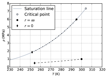
Figure 2: The pressure profiles of the isentropic vortex case, plotted in relation to the saturation pressure of $\text{CO}_{\text{2}}$. The pressure in the single-phase case is drawn as a dashed line and the pressure in the two-phase case is drawn as a dash-dotted line.

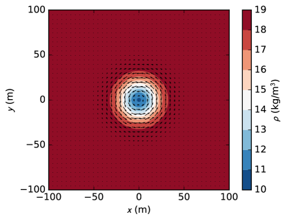
Figure 3: Density contours of the single-phase isentropic vortex case. The fluid circulates around the central low-pressure region.

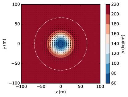
Figure 4: Density contours of the two-phase isentropic vortex case. The fluid is in a pure gas state at $r=\infty$, but condenses and enters a gas-liquid state near the centre of the vortex due to the lower pressure. The white dashed line indicates a liquid volume fraction of ${10}^{-12}\text{\,}\text{/}$.

It is important to note that in setting the state variables in each cell initially, we must calculate the state variables at every quadrature point in the cell and then take the average. Using only one quadrature point per cell results in a second-order error in the initial condition. The simulations were run to $t=$0.1\text{\,}\mathrm{s}\text{/}$$ in a square domain $[-100,100]\times[-100,100]\,$\mathrm{m}\text{/}$$ with periodic boundary conditions and with a CFL number $C_{\text{CFL}}=0.45$. For comparison, reconstruction in both the set $\boldsymbol{W}=\left[e,\rho,u_{x},u_{y}\right]$ and in the local characteristic variables (see A) was performed.

Table 2: Errors in the density field and estimated convergence orders in the single-phase isentropic vortex case (i) with the PR EOS and reconstruction in local characteristic variables.

Grid	$L_{1}$-error	$L_{1}$-order	$L_{\infty}$-error	$L_{\infty}$-order
$25\times 25$	$1.286\text{\times}{10}^{-02}\text{\,}\text{/}$	-	$1.432\text{\times}{10}^{-01}\text{\,}\text{/}$	-
$50\times 50$	$5.975\text{\times}{10}^{-04}\text{\,}\text{/}$	$4.43\text{\,}\text{/}$	$1.008\text{\times}{10}^{-02}\text{\,}\text{/}$	$3.83\text{\,}\text{/}$
$100\times 100$	$2.044\text{\times}{10}^{-05}\text{\,}\text{/}$	$4.87\text{\,}\text{/}$	$3.760\text{\times}{10}^{-04}\text{\,}\text{/}$	$4.74\text{\,}\text{/}$
$200\times 200$	$7.410\text{\times}{10}^{-07}\text{\,}\text{/}$	$4.79\text{\,}\text{/}$	$1.140\text{\times}{10}^{-05}\text{\,}\text{/}$	$5.04\text{\,}\text{/}$

Table 3: Errors in the density field and estimated convergence orders in the single-phase isentropic vortex case (i) with the PR EOS and reconstruction in $\boldsymbol{W}=[e,\rho,u_{x},u_{y}]$.

Grid	$L_{1}$-error	$L_{1}$-order	$L_{\infty}$-error	$L_{\infty}$-order
$25\times 25$	$1.314\text{\times}{10}^{-02}\text{\,}\text{/}$	-	$1.532\text{\times}{10}^{-01}\text{\,}\text{/}$	-
$50\times 50$	$6.468\text{\times}{10}^{-04}\text{\,}\text{/}$	$4.34\text{\,}\text{/}$	$1.225\text{\times}{10}^{-02}\text{\,}\text{/}$	$3.64\text{\,}\text{/}$
$100\times 100$	$2.196\text{\times}{10}^{-05}\text{\,}\text{/}$	$4.88\text{\,}\text{/}$	$3.722\text{\times}{10}^{-04}\text{\,}\text{/}$	$5.04\text{\,}\text{/}$
$200\times 200$	$8.070\text{\times}{10}^{-07}\text{\,}\text{/}$	$4.77\text{\,}\text{/}$	$1.254\text{\times}{10}^{-05}\text{\,}\text{/}$	$4.89\text{\,}\text{/}$

Table 4: Errors in the density field and estimated convergence orders in the two-phase isentropic vortex case (ii) with the PR EOS and reconstruction in the local characteristic variables.

Grid	$L_{1}$-error	$L_{1}$-order	$L_{\infty}$-error	$L_{\infty}$-order
$25\times 25$	$1.398\text{\times}{10}^{-01}\text{\,}\text{/}$	-	$1.775\text{\times}{10}^{00}\text{\,}\text{/}$	-
$50\times 50$	$8.523\text{\times}{10}^{-03}\text{\,}\text{/}$	$4.04\text{\,}\text{/}$	$1.365\text{\times}{10}^{-01}\text{\,}\text{/}$	$3.70\text{\,}\text{/}$
$100\times 100$	$3.048\text{\times}{10}^{-04}\text{\,}\text{/}$	$4.81\text{\,}\text{/}$	$5.926\text{\times}{10}^{-03}\text{\,}\text{/}$	$4.53\text{\,}\text{/}$
$200\times 200$	$1.119\text{\times}{10}^{-05}\text{\,}\text{/}$	$4.77\text{\,}\text{/}$	$3.183\text{\times}{10}^{-04}\text{\,}\text{/}$	$4.22\text{\,}\text{/}$

Table 5: Errors in the density field and estimated convergence orders in the two-phase isentropic vortex case (ii) with the PR EOS and reconstruction in $\boldsymbol{W}=[e,\rho,u_{x},u_{y}]$.

Grid	$L_{1}$-error	$L_{1}$-order	$L_{\infty}$-error	$L_{\infty}$-order
$25\times 25$	$1.615\text{\times}{10}^{-01}\text{\,}\text{/}$	-	$1.976\text{\times}{10}^{00}\text{\,}\text{/}$	-
$50\times 50$	$9.200\text{\times}{10}^{-03}\text{\,}\text{/}$	$4.13\text{\,}\text{/}$	$1.591\text{\times}{10}^{-01}\text{\,}\text{/}$	$3.63\text{\,}\text{/}$
$100\times 100$	$3.314\text{\times}{10}^{-04}\text{\,}\text{/}$	$4.80\text{\,}\text{/}$	$6.635\text{\times}{10}^{-03}\text{\,}\text{/}$	$4.58\text{\,}\text{/}$
$200\times 200$	$1.215\text{\times}{10}^{-05}\text{\,}\text{/}$	$4.77\text{\,}\text{/}$	$2.522\text{\times}{10}^{-04}\text{\,}\text{/}$	$4.72\text{\,}\text{/}$

The errors in the density field and the estimated convergence orders for the single-phase case (i) are presented in Table 2 for reconstruction in the local characteristic variables and in Table 3 for reconstruction in $\boldsymbol{W}$. It is observed that reconstruction in the characteristic variables, although much more computationally expensive, produces an error that is of the same order of magnitude as reconstruction in $\boldsymbol{W}$. The general trend is that the errors obtained with characteristic reconstruction are slightly lower. The difference is small, however, and only about 8% in the $L_{1}$-norm on the $200\times 200$ grid. High-order convergence was obtained with both reconstruction options and significant oscillations were not observed in any simulations of this case.

Despite using a third-order RK method and a fourth-order quadrature rule, we get close to fifth-order convergence with both reconstruction alternatives. Similar behaviour was also observed by Titarev and Toro [11] and by Coralic and Colonius [13] and suggests that the error in the time integration method is small compared to that of the spatial discretization in this case.

We have also considered a three-dimensional, single-phase isentropic vortex problem with rotation in the $x$-$z$ plane. These results also showed close to fifth-order convergence and are omitted here.

The errors in the density field and the estimated convergence orders for the two-phase case (ii) are presented in Table 4 for reconstruction in the local characteristic variables and in Table 5 for reconstruction in $\boldsymbol{W}$. Again, the general trend is that the errors are slightly smaller for reconstruction in the local characteristic variables than for reconstruction in $\boldsymbol{W}$, but again the differences are small. For this case, the difference is about $0.5\text{\,}\mathrm{\char 37\relax}\text{/}$ in the $L_{1}$-norm on the $200\times 200$ grid, while the error in the $L_{\infty}$-norm on the same grid is smaller with reconstruction in $\boldsymbol{W}$. As for the single-phase case, no significant oscillations were observed and the errors show close to fifth-order covergence.

We have also performed simulations of both case (i) and case (ii) using the more complex SW EOS, in place of the PR EOS, and reconstruction in $\boldsymbol{W}$. The errors and convergence orders are shown in Table 6 and Table 7 respectively. For both cases, the results are similar to those obtained with the PR EOS (see Table 3 and Table 5). This indicates that the order of the numerical method is not affected by the degree of complexity of the EOS underlying the phase equilibrium calculations.

Table 6: Errors in the density field and estimated convergence orders in the single-phase isentropic vortex case (i) with the SW EOS and reconstruction in $\boldsymbol{W}=[e,\rho,u_{x},u_{y}]$.

Grid	$L_{1}$-error	$L_{1}$-order	$L_{\infty}$-error	$L_{\infty}$-order
$25\times 25$	$1.303\text{\times}{10}^{-2}\text{\,}\text{/}$	-	$1.518\text{\times}{10}^{-1}\text{\,}\text{/}$	-
$50\times 50$	$6.391\text{\times}{10}^{-4}\text{\,}\text{/}$	$4.35\text{\,}\text{/}$	$1.207\text{\times}{10}^{-2}\text{\,}\text{/}$	$3.65\text{\,}\text{/}$
$100\times 100$	$2.175\text{\times}{10}^{-5}\text{\,}\text{/}$	$4.88\text{\,}\text{/}$	$3.663\text{\times}{10}^{-4}\text{\,}\text{/}$	$5.04\text{\,}\text{/}$
$200\times 200$	$8.001\text{\times}{10}^{-7}\text{\,}\text{/}$	$4.76\text{\,}\text{/}$	$1.236\text{\times}{10}^{-5}\text{\,}\text{/}$	$4.89\text{\,}\text{/}$

Table 7: Errors in the density field and estimated convergence orders in the two-phase isentropic vortex case (ii) with the SW EOS and reconstruction in $\boldsymbol{W}=[e,\rho,u_{x},u_{y}]$.

Grid	$L_{1}$-error	$L_{1}$-order	$L_{\infty}$-error	$L_{\infty}$-order
$25\times 25$	$2.008\text{\times}{10}^{-1}\text{\,}\text{/}$	-	$2.402\text{\,}\text{/}$	-
$50\times 50$	$1.150\text{\times}{10}^{-2}\text{\,}\text{/}$	$4.13\text{\,}\text{/}$	$1.983\text{\times}{10}^{-1}\text{\,}\text{/}$	$3.60\text{\,}\text{/}$
$100\times 100$	$4.081\text{\times}{10}^{-4}\text{\,}\text{/}$	$4.82\text{\,}\text{/}$	$7.891\text{\times}{10}^{-3}\text{\,}\text{/}$	$4.65\text{\,}\text{/}$
$200\times 200$	$1.467\text{\times}{10}^{-5}\text{\,}\text{/}$	$4.80\text{\,}\text{/}$	$3.055\text{\times}{10}^{-4}\text{\,}\text{/}$	$4.69\text{\,}\text{/}$

To summarize, close to fifth-order convergence is observed in both the single-phase (i) and the two-phase (ii) isentropic vortex cases. This demonstrates that the high-order convergence of the numerical methods is not limted to single-phase problems with simple EOS. The results also suggest that in this case, errors in third-order temporal integration and fourth-order quadrature rules are not dominating. Differences in the error between reconstruction in $\boldsymbol{W}$ and local characteristic variables are small. As reconstruction in $\boldsymbol{W}$ is much less computationally intensive, it may be preferable in cases where the more advanced option is not needed in order to avoid oscillations.

5.3 Double Mach reflection of strong shock

Next we consider a double Mach reflection of a strong shock incident on a planar wall. This problem tests the ability of the numerical methods, and their implementation, to handle strong shocks. This type of reflection problems was designed to mimic experiments where a shock propagates down a tube and hits an inserted wedge. The flow pattern resulting from the reflection of the shock on the wedge is complicated and challenging to simulate numerically. In particular, the forward jet that forms along the wall behind the first Mach stem (from approximately $x=$2.3\text{\,}\mathrm{m}\text{/}$$ to $x=$2.8\text{\,}\mathrm{m}\text{/}$$ in Figure 5) is difficult to resolve [38].

To have results that could be compared with those from the literature, the simulation was run with parameters that seem to be the most common, e.g. the parameters used by Titarev and Toro [11]. This also implies the ideal-gas EOS and adiabatic constant $\gamma=1.4$.

We consider a domain $[0,4]\times[0,1]\,$\mathrm{m}\text{/}$$. A shock is initiated with a right-moving Mach 10 front incident on the $x$-axis at $x=$1\text{/}6\text{\,}\mathrm{m}\text{/}$$ and a forward angle of $60^{\circ}$. The undisturbed region in front of the shock is at rest with $p=$1\text{\,}\mathrm{Pa}\text{/}$$ and $\rho=$1.4\text{\,}\mathrm{k}\mathrm{g}\mathrm{/}\mathrm{m}^{3}$$. In post-shock region the fluid moves with velocities $u_{y}=$-4.125\text{\,}\mathrm{m}\text{/}\mathrm{s}$$ and $u_{x}=-\sqrt{3}u_{y}$, and has $p=$116.5\text{\,}\mathrm{Pa}\text{/}$$ and $\rho=$8.0\text{\,}\mathrm{k}\mathrm{g}\mathrm{/}\mathrm{m}^{3}$$.

The south wall is reflecting for $x\geq$1\text{/}6\text{\,}\mathrm{m}\text{/}$$ and has post-shock values for $x<$1\text{/}6\text{\,}\mathrm{m}\text{/}$$. The eastern boundary has a zero-gradient boundary condition and the western boundary carries post shock values. The northern boundary is dynamic with post-shock values in the post-shock region and undisturbed values in the undisturbed region. For further details on the problem and how it is defined, the reader is referred to Woodward and Colella [38]. A note on the setup of the case is given by Kemm [39].

We use a CFL number of $C_{\text{CFL}}=0.4$ and a grid size of $1920\times 480$. To avoid spurious oscillations, it was necessary to perform reconstruction in the local characteristic variables for this case (see A).

A contour plot of the density at $t=$0.2\text{\,}\mathrm{s}\text{/}$$ is shown in Figure 5. We observe that both Mach stems (starting at about $x=$0.15\text{\,}\mathrm{m}\text{/}$$ and $x=$2.8\text{\,}\mathrm{m}\text{/}$$) are sharp and that the details of the jet structure (in the lower part of the figure around $x=$2.5\text{\,}\mathrm{m}\text{/}$$) are well-resolved. The positions of the shocks and discontinuities compare well with results from the literature [38, 12, 40, 11]. The same is true for the positions of the isodensity lines and the level of detail obtained here, compared to the fifth-order WENO reconstruction scheme on the same grid size in [11]. We conclude that the solution obtained here is in good agreement with that which is generally accepted in the literature.

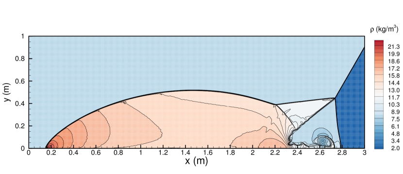
(a) Whole flow field

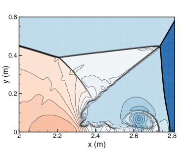
(b) Close-up

Figure 5: Contour plot of density in the double Mach reflection problem. Thirty contour lines in the range $\left[$2\text{\,}\mathrm{k}\mathrm{g}\mathrm{/}\mathrm{m}^{3}$,$22\text{\,}\mathrm{k}\mathrm{g}\mathrm{/}\mathrm{m}^{3}$\right]$ are used.

5.4 Air jet flow from rectangular nozzle

The present validation test consists of a 3D direct numerical simulation of a transitional subsonic air jet issuing from a rectangular nozzle into quiescent air. The chosen configuration (with air modelled as an ideal gas) is computationally less expensive than the main demonstration case of the present paper, the supersonic CO2 jet with complex thermodynamic behaviour (Section 6). It retains, however, some of its general flow features and, due to its straightforward boundary condition specification, can be conveniently compared with experimental data presented by Deo et al. [41].

The air jet issues with a centreline velocity of $u_{y,\text{c},0}=$26.3\text{\,}\mathrm{m}\text{/}\mathrm{s}$$ into initially quiescent air at a temperature of $293\text{\,}\mathrm{K}\text{/}$ and pressure of $1\text{\,}\mathrm{atm}\text{/}$. The nozzle configuration consists of a rectangular slot of dimensions $w\times h$ characterized by high aspect ratio $w/h\sim 10$ where $h=$5.6\text{\,}\mathrm{mm}\text{/}$$, as in [41], resulting in a jet Reynolds number $\mathit{Re}_{jet}=\rho u_{y,\text{c},0}h/\eta\sim${10}^{5}$$. Furthermore, the imposed jet inlet velocity distribution follows a “top-hat” profile to reproduce the effects of a conventional smoothly-contracting nozzle shape with laminar boundary layers, as discussed in [41]. For the experimental conditions that are targeted in the present work, the jet’s own turbulent velocity fluctuations are considered relatively unimportant and no velocity perturbations are introduced at the jet inlet. Natural perturbations of the acoustic field, intrinsically represented by the present compressible formulation, are sufficient to cause the jet flow to become unstable and break-up. The direction of the jet flow is in the positive $y$-direction. The two-dimensionality of the jet at the inlet nozzle is ensured by a periodic boundary condition in the spanwise direction z to eliminate border effects. Open, non-reflecting boundary conditions are imposed at the upper $y$ boundary and at both $x$ boundaries.

Figure 6 presents a visualization of the three-dimensional computational domain and a snapshot of the flow at $t=$35\text{\,}\mathrm{ms}\text{/}$$. The domain extends $L_{y}=$20\text{\,}\mathrm{cm}\text{/}$$ in the $x$- and $y$-directions and $5\text{\,}\mathrm{cm}\text{/}$ in the $z$-direction. The computational domain is discretized by $400\times 400\times 100$ grid nodes in the $x$-, $y$- and $z$-direction, respectively. This gives a constant spatial resolution of $0.5\text{\,}\mathrm{mm}\text{/}$ throughout the computational domain and implies that the jet inlet dimension $h$ is resolved by twelve grid nodes, while $C_{\text{CFL}}=0.3$ in this three-dimensional simulation.

Figure 6: Air jet: Visualization of the flow and computational domain. The yellow colour indicates the $2500\text{\,}\text{/}\mathrm{s}$ vorticity magnitude.

After the simulation is started, a settling time approximately equal to $t_{\text{ini}}\sim L_{y}/u_{y,\text{c},0}=$7.6\text{\,}\mathrm{ms}\text{/}$$ is allowed in order to ensure that the initial transient is transported outside of the computational domain. The time step is allowed to adapt to the varying CFL conditions. After the initial transient, however, it is observed that it stabilizes around $\Delta t\sim$0.4\text{\,}\mathrm{\SIUnitSymbolMicro s}\text{/}$$. Sampling of the solution is started for $t>t_{\text{ini}}$, every 500 time steps or $0.2\text{\,}\mathrm{ms}\text{/}$ (corresponding approximately to the characteristic jet time $t_{\text{jet}}=h/u_{y,\text{c},0}$). Sampling is stopped at $t_{\text{end}}=$50\text{\,}\mathrm{ms}\text{/}$$ after approximately 5.5 domain transit times and 238 characteristic jet times $t_{\text{jet}}$. Figure 7(a) illustrates the spatial pattern of the mean jet (wall-normal) velocity component that is averaged in time and in the homogeneous spanwise direction ($z$) and normalized by the centreline jet exit velocity $u_{y,\text{c},0}$. Figure 7(b) analogously shows the normalized root mean square of the velocity fluctuation in the jet direction. The typical features of jet flows are present with a clearly visible potential core ($u_{y}\sim u_{y,\text{c},0}$) characterized by low level of velocity fluctuations. Downstream of it, as the jet spreads, the velocity fluctuations increase due to entrainment of the surrounding air and jet break-up.

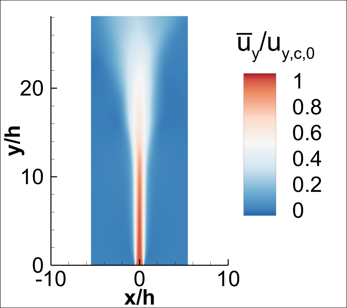
(a) Average of the velocity component in the jet direction, $\bar{u}_{y}$.

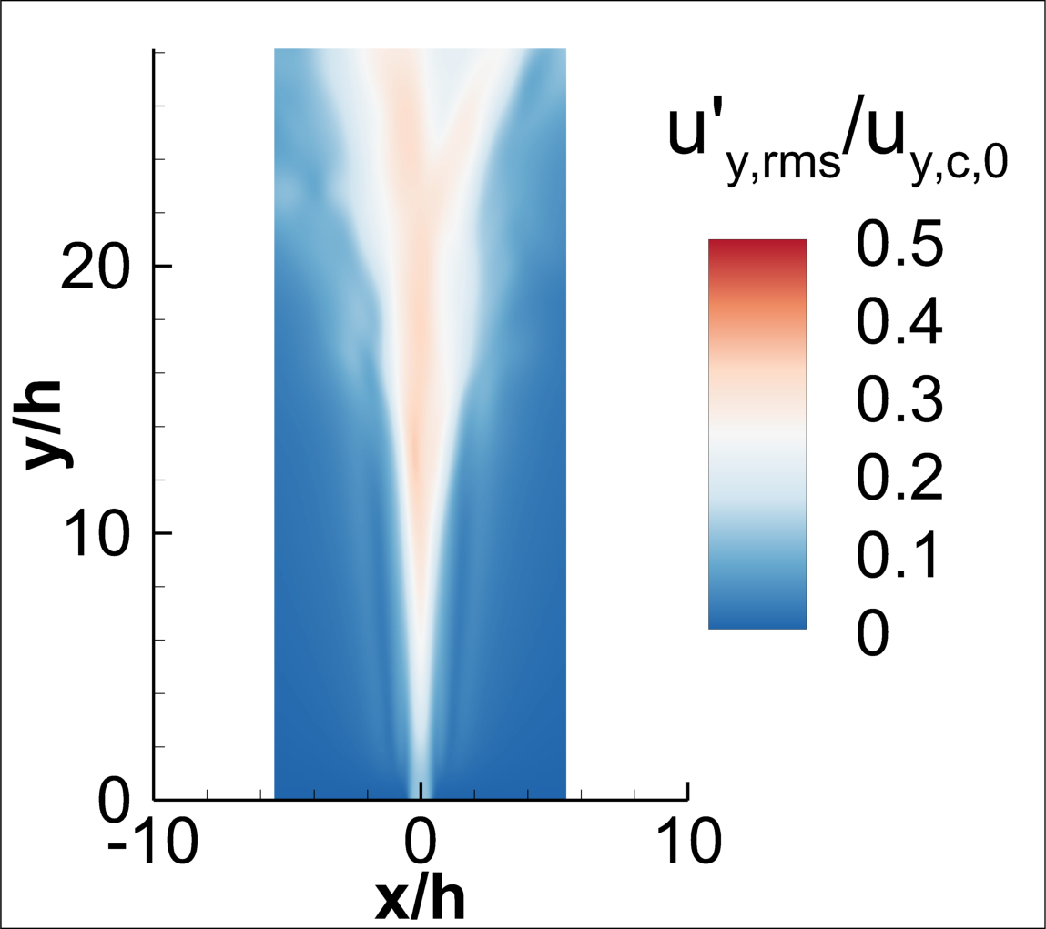
(b) Average of the root mean square of the velocity fluctuation $u^{\prime}_{y,\text{rms}}$ in the jet direction.

Figure 7: Air jet: Pointwise temporal and spatial (in $z$-direction) average velocity quantities, normalized by the centreline value at the nozzle exit, $u_{y,\text{c},0}$.

Figure 8 provides a more quantitative measure of the spatial extent of the potential core and of the characteristic mean velocity decay in the region of self-similarity. The length of the potential core, equal to $4h$, is in very good accordance with the values reported by Deo et al. [41]. Furthermore, the characteristic $1/2$-power law inverse decay can also be clearly observed, indicating a statistically two-dimensional behaviour of the jet, together with the appearance, further downstream, of the inversely-linear decay that indicates transition to a (more three-dimensional) axisymmetric form [41]. As pointed out in [41], the logarithmic scale used in the abscissa is essential to identify the points of transition from statistically two-dimensional to three-dimensional mean flow. Although a considerable spread in the specific spatial location of this transition is present in the available data, see Figures 6 and 7 in [41], the present results are consistent with the observed trend that the transition is delayed for increasing slot aspect ratios and anticipated for decreasing ones. The present aspect ratio $w/h$ is approximately 10 with the transition starting 20 nozzle widths $h$ downstream of the jet inlet, while for the aspect ratios of 30 and 60 investigated experimentally by [41], the same transition starts at 30 and 50 nozzle widths $h$ downstream of the jet inlet. Finally, it is worth noticing the very good accordance between the present results and the results presented in Figure 7 of [41] with respect to the spatial evolution of the centreline velocity fluctuations, see Figure 9: the rapid increase for $y/h$ between 0 and 10, the peak located between 10 and 20 and the following decay.

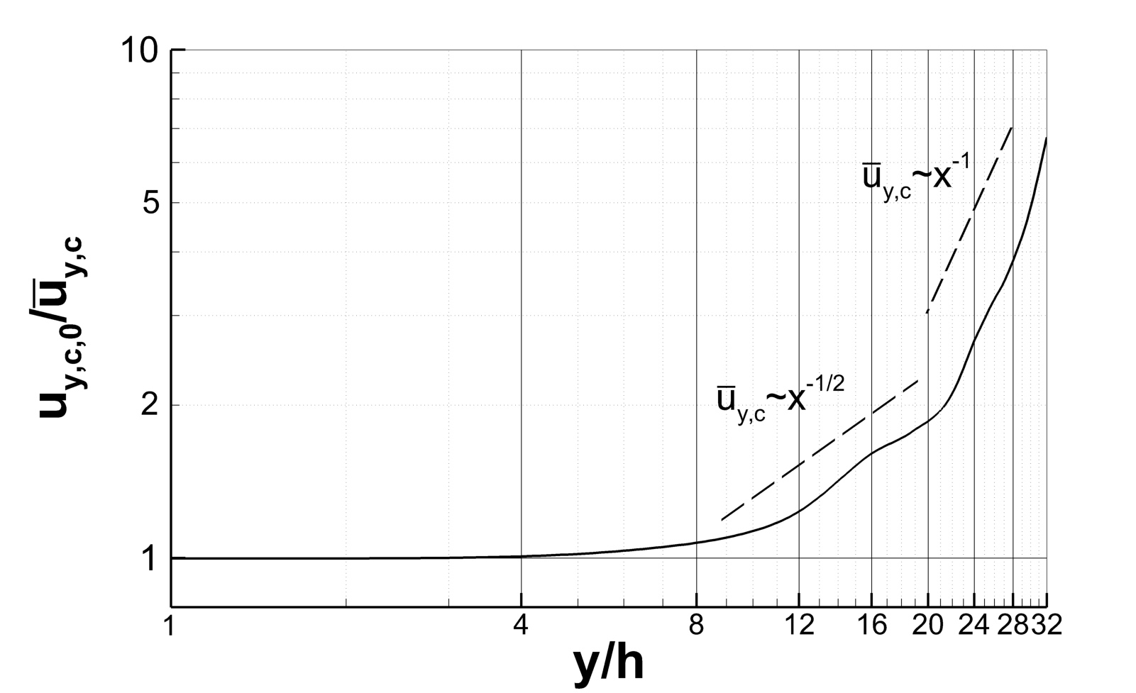
Figure 8: Air jet: 1D profile of the normalized centreline mean jet velocity $u_{y,\text{c},0}/\bar{u}_{y}$ illustrating the well-known decay rates in the jet self-similar region.

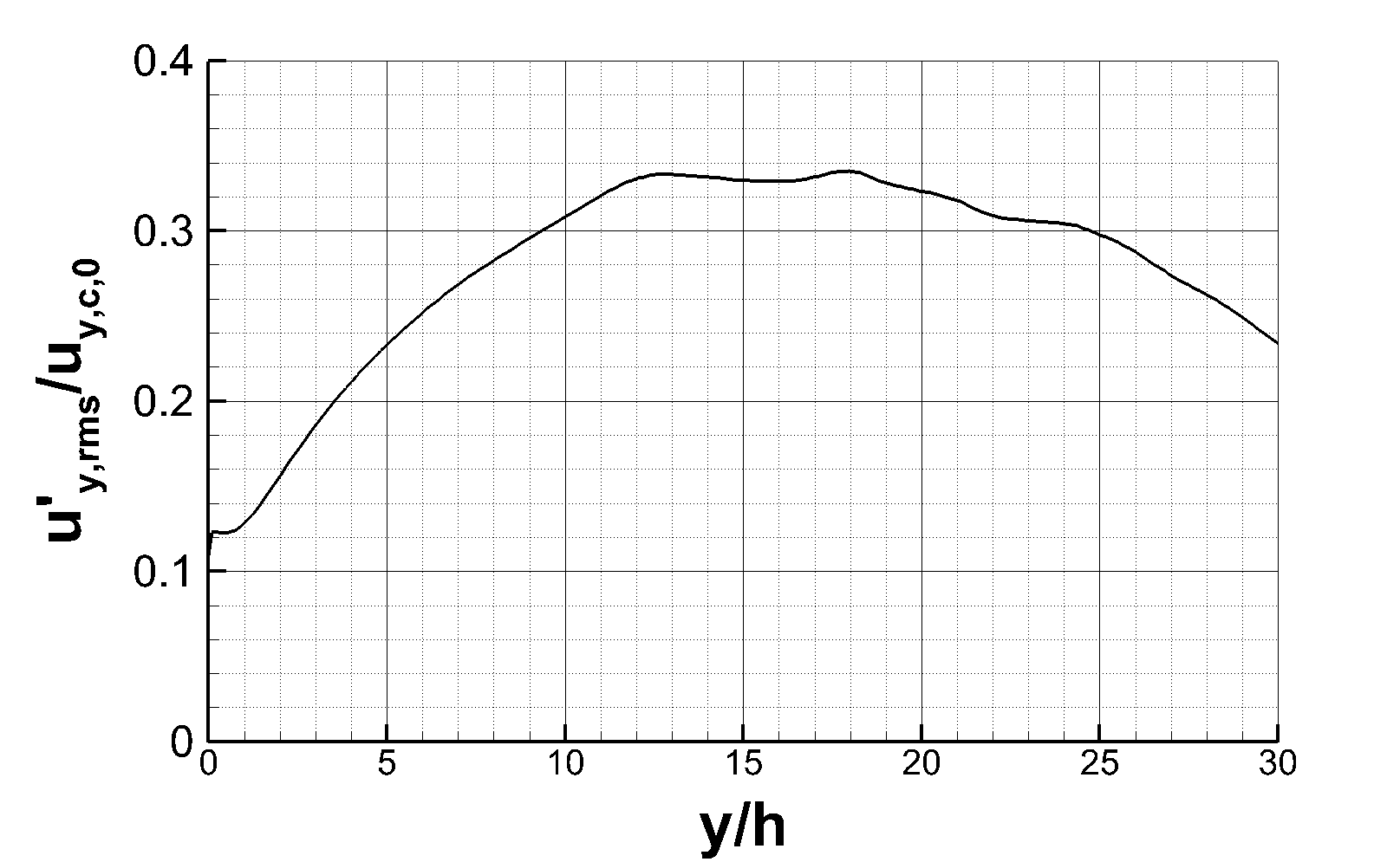
Figure 9: Air jet: 1D profile of the normalized fluctuating jet velocity $u^{\prime}_{y,\text{rms}}/u_{y,\text{c},0}$ illustrating the well-known decay rates in the jet self-similar region and peak in the turbulent fluctuations for $y/h\sim 10$.

Figure 10 complements the previous analysis by providing insight into the time-dependent behaviour of the flow structure in the near field. The power spectrum (distribution of the energy of a waveform among its different frequency components) of the fluctuating instantaneous velocity is obtained through a discrete Fourier transform and plotted versus the frequency, normalized by the characteristic frequency defined as $1/t_{\text{jet}}=u_{y,\text{c},0}/h$ for a sampling location within the potential core region (at $y/h=3$). The presence of broad peaks in the spectrum indicates the generation of regularly-occurring large-scale coherent vortices, a well-known feature of jet flows. Furthermore, the observed decay of approximately two orders of magnitude in the spectrum is consistent with the experimental observations described in [41].

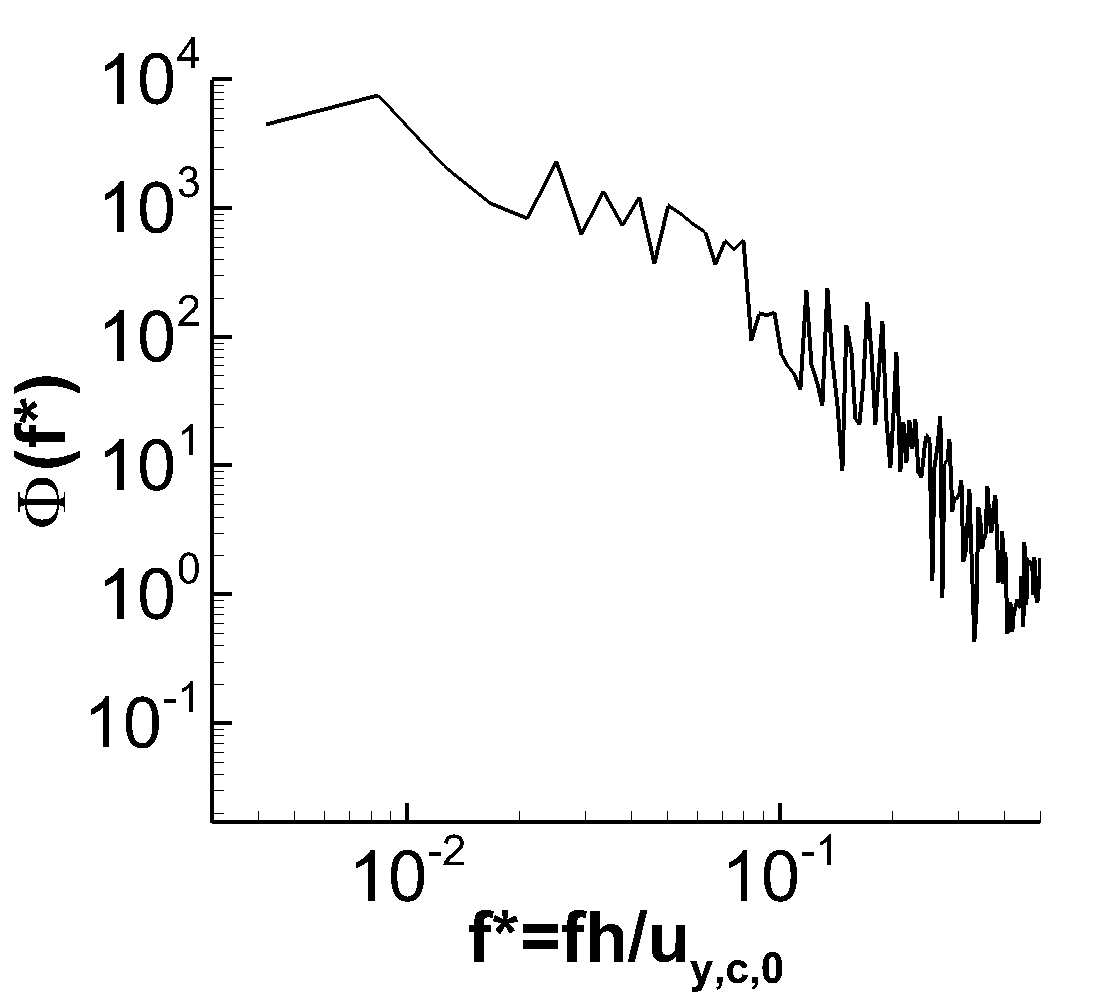
Figure 10: Air jet: Power spectrum of the instantaneous velocity sampled at $y/h=3$ on the centreline of the jet potential core.

In summary, the method seems able to accurately capture the main features of transitional planar jets at the resolution employed in the present test.

6 Simulation of $\text{CO}_{\text{2}}$ jet

As an application of our method, we now consider two cases involving high-speed flow of $\text{CO}_{\text{2}}$, including phase change and three-phase (gas-liquid-solid) flow.

6.1 Case A

Some relevant experimental data were presented by Li et al. [42], and we focus on the case labelled “RHP = 0.030”, see Figure 13.

6.1.1 Case description

Stagnant pure $\text{CO}_{\text{2}}$ of temperature $T=$40\text{\,}\mathrm{\SIUnitSymbolCelsius}\text{/}$$ and pressure $p=$52.2\text{\,}\mathrm{bar}\text{/}$$ is expanded through a round hole of diameter $d_{\text{e}}=$1\text{\,}\mathrm{mm}\text{/}$$. We consider that $\text{CO}_{\text{2}}$ has replaced air in the vicinity of the jet, so the initial condition in the computational domain is stagnant $\text{CO}_{\text{2}}$ of temperature $T_{0}=$20\text{\,}\mathrm{\SIUnitSymbolCelsius}\text{/}$$ and pressure $p_{0}=$1\text{\,}\mathrm{bar}\text{/}$$. At $t=$0\text{\,}\mathrm{s}\text{/}$$, the $\text{CO}_{\text{2}}$ starts flowing through the hole. The jet is highly underexpanded and starts forming a barrel shock, which attains a steady state after about $t=$0.25\text{\,}\mathrm{ms}\text{/}$$. The Reynolds number at the inlet is $6\text{\times}{10}^{5}$.

In this case, the thermodynamic properties of pure $\text{CO}_{\text{2}}$ are calculated as described in Section 2.2, with the SW EOS. The thermal conductivity is set to $0.0145\text{\,}\mathrm{W}\text{/}\text{(}\mathrm{m}\text{\,}\mathrm{K}\text{)}$.

6.1.2 Computational set-up

The computational domain, shown in Figure 11, is a cube of edge length $5\text{\,}\mathrm{cm}\text{/}$, divided into an equidistant grid. The hole geometry is represented by a Cartesian approximation and the inflow condition is described in Section 3.1. At the inlet edge, the boundary condition outside the hole is a no-slip wall. The other boundaries are governed by the NSCBC (see Section 3.2) employing a far-field pressure of $1\text{\,}\mathrm{bar}\text{/}$ and an $\alpha$-coefficient of 10.0. Here, the jet flow is in the $y$ direction.

Figure 11: $\text{CO}_{\text{2}}$ jet A: Computational domain including the steady-state $\mathit{Ma}=2.5$ isocontour in red. The inlet is in the middle of the $x$-$z$ plane.

Two grids were employed, with $200^{3}$ and $400^{3}$ cells. In the latter case, the inlet hole had eight cells across the diameter. The computations were performed using the fourth-order accurate quadrature rule (see Section 4.1) with the WENO scheme and $C_{\text{CFL}}=0.333$. In the WENO scheme, the internal energy, density and velocity were used as reconstruction variables, and this combination was found to work well.

6.1.3 Results

Pressure contours of the developing barrel shock are displayed in Figure 12, while Figure 14(a) shows Mach-number contours at $t=$0.5\text{\,}\mathrm{ms}\text{/}$$. In the computation, the state is gas-liquid-solid in a small region close to the nozzle exit. The gas-solid state is found in a larger region, particularly inside the barrel shock, but there is also some solid in the zone beyond the barrel shock. This is illustrated in Figure 14(b). In the figure, the solid mass fraction is indicated by the different coloured contours, while the liquid area, appearing near the inlet, is denoted by green colour, which is the $1\text{\,}\mathrm{\char 37\relax}\text{/}$ isocontour of the liquid mass fraction. Although quantitative measurements are not available in Li et al. [42], we expect the present method to underestimate the post-shock solid mass fraction in this case due to the assumption of full thermodynamic equilibrium.

Temperature contours are shown in Figure 14(c). It can be seen that the $\text{CO}_{\text{2}}$ jet core is at about $-70\text{\,}\mathrm{\SIUnitSymbolCelsius}\text{/}$, while the coldest temperature, about $-100\text{\,}\mathrm{\SIUnitSymbolCelsius}\text{/}$, is appearing right before the Mach disk, due to the strong expansion.

(a) $t=$10\text{\,}\mathrm{\SIUnitSymbolMicro s}\text{/}$$.

(b) $t=$20\text{\,}\mathrm{\SIUnitSymbolMicro s}\text{/}$$.

(c) $t=$30\text{\,}\mathrm{\SIUnitSymbolMicro s}\text{/}$$.

(d) $t=$40\text{\,}\mathrm{\SIUnitSymbolMicro s}\text{/}$$.

Figure 12: $\text{CO}_{\text{2}}$ jet A: Pressure contours of the developing shock. Plane through $z=$0.025\text{\,}\mathrm{m}\text{/}$$. $400^{3}$ computational cells.

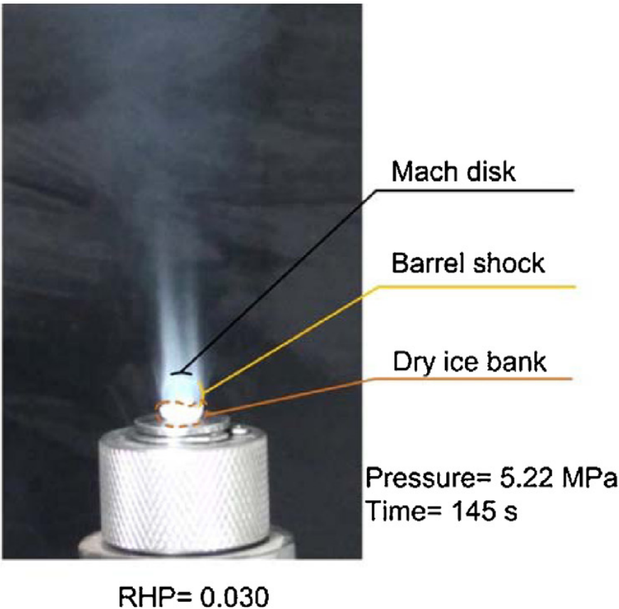
Figure 13: Photograph of $\text{CO}_{\text{2}}$ jet A. Reprinted from Figure 7 in Li et al. [42], copyright (2016), with permission from Elsevier.

(a) Mach number.

(b) Solid mass fraction. Liquid appears in the green area near the inlet.

(c) Temperature.

(d) Logarithmic density. $\rho_{0}=$1.82\text{\,}\mathrm{kg}\text{/}{\mathrm{m}}^{3}$$ corresponds to the initial state.

Figure 14: $\text{CO}_{\text{2}}$ jet A: Snapshots at $0.5\text{\,}\mathrm{ms}\text{/}$, where the barrel shock is in a steady state. Plane through $z=$0.025\text{\,}\mathrm{m}\text{/}$$. $200^{3}$ computational cells.

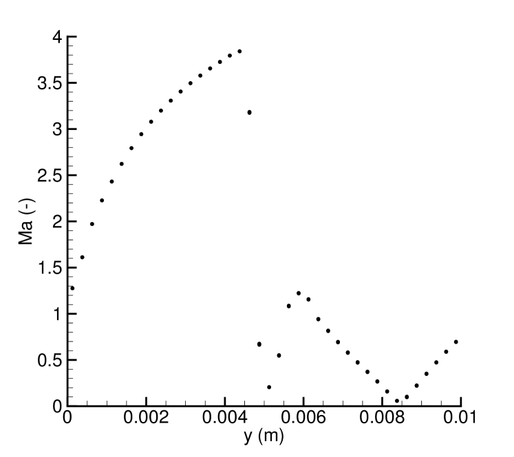
(a) Mach number.

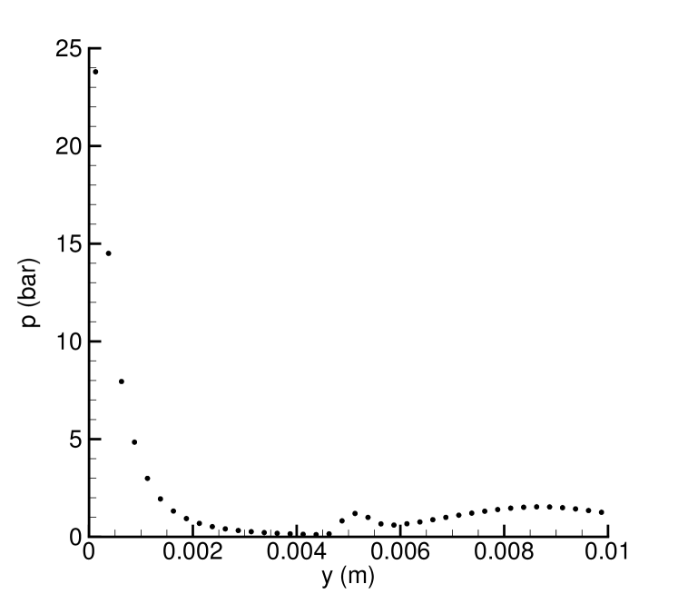
(b) Pressure.

Figure 15: $\text{CO}_{\text{2}}$ jet A: Mach number and pressure plotted along the jet centreline at $0.5\text{\,}\mathrm{ms}\text{/}$.

In Figure 15, the Mach number and the pressure are plotted along the jet centreline. It can be seen that the position of the Mach disk is $l_{\text{MD}}=$4.8\text{\,}\mathrm{mm}\text{/}$$. This position can also be estimated by the correlation recommended by Franquet et al. [43]:

$$l_{\text{MD}}=d_{\text{e}}\sqrt{\frac{p/p_{0}}{2.4}}\approx$4.7\text{\,}\mathrm{mm}\text{/}$.$$ (32)

This is in good agreement with the present result.

An accurate position of the Mach disk cannot be obtained from the photograph in Figure 13 or the description in Li et al. [42]. However, we estimate that the position of the Mach disk is roughly at half a centimetre in that photograph. Thus there is good agreement between the photograph and the present result. Further, in Figure 14(a), it can be seen that the boundary layer around the jet starts widening at about $4\text{\,}\mathrm{cm}\text{/}$. This is also in agreement with Figure 13. However, in that photograph, one can see ice at the nozzle exit, labelled “dry ice bank”. In view of the high $\text{CO}_{\text{2}}$ exit velocity, we find it unlikely that dry-ice particles deposit immediately at the exit. The ice may well be frozen moisture from the surrounding air.

6.2 Case B

Finally, we consider the $\text{CO}_{\text{2}}$ jet presented as Test B in Pursell [44].

6.2.1 Case description and computational set-up

The set-up is analogous to that in Case A, except that the orifice diameter is four times larger. The inlet condition corresponds to saturated gas. Pure $\text{CO}_{\text{2}}$ of temperature $T=$-3.5\text{\,}\mathrm{\SIUnitSymbolCelsius}\text{/}$$ and pressure $p=$31.0\text{\,}\mathrm{bar}\text{/}$$ is expanded through a round hole of diameter $d_{\text{e}}=$4\text{\,}\mathrm{mm}\text{/}$$. The Reynolds number at the inlet is $2\text{\times}{10}^{6}$. The initial temperature in the computational domain is assumed to be $T_{0}=$20\text{\,}\mathrm{\SIUnitSymbolCelsius}\text{/}$$.

The computational domain is a cube of edge length $10\text{\,}\mathrm{cm}\text{/}$, divided into an equidistant grid with 200 cells in each direction.

6.2.2 Results

Figure 16 shows contours of the absolute velocity plotted at $t=$0.28\text{\,}\mathrm{ms}\text{/}$$. The Mach-disk position is at $16.1\text{\,}\mathrm{mm}\text{/}$ and the width of the structure is $21.7\text{\,}\mathrm{mm}\text{/}$. In this case, the correlation (32) gives $l_{\text{MD}}\approx$14.4\text{\,}\mathrm{mm}\text{/}$$ for the Mach-disk position, which is a difference of $12\text{\,}\mathrm{\char 37\relax}\text{/}$ – somewhat larger than in Case A.

The experimental values found by Pursell [44] are $17.8\text{\,}\mathrm{mm}\text{/}$ and $21.9\text{\,}\mathrm{mm}\text{/}$, for the Mach-disk position and the ‘effective diameter’, respectively. Hence, the simulated Mach-disk position lies between that measured by Pursell and the one given by the correlation. The agreement is very good between the simulated and measured effective diameter. Further, the barrel-shock structure seen in Figure 16 closely corresponds to the photograph given in Figure 5(b) in Pursell [44].

Figure 16: $\text{CO}_{\text{2}}$ jet B: Absolute velocity in a plane through $z=$0.025\text{\,}\mathrm{m}\text{/}$$. Snapshot at $t=$0.28\text{\,}\mathrm{ms}\text{/}$$.

7 Conclusions

We have developed a high-order finite-volume method capable of handling single-phase, two-phase (gas-liquid) and three-phase (gas-solid-liquid) flow with discontinuities. The spatial and temporal discretization is similar to that of Coralic and Colonius [13], employing a fifth-order WENO scheme and a third-order strong-stability-preserving Runge–Kutta method. In the present case, however, the model formulation is based on the homogeneous equilibrium model. The fluid phase behaviour is calculated using a suitable EOS and assuming full local thermodynamic equilibrium. This approach requires special care in the implementation of the flash algorithms required to translate the state variables into primitive variables.

The method has been validated using various benchmark cases, showing robust behaviour and high-order convergence for smooth single- and two-phase flow. Further, the calculation of a turbulent air jet was validated by comparing with data from Deo et al. [41]. Finally, the method was employed to calculate a highly underexpanded $\text{CO}_{\text{2}}$ jet exhibiting phase transition and three-phase flow. To this end, the Span and Wagner [21] reference EOS was employed. The method was able to robustly and accurately capture the complex and intertwined thermo- and fluid dynamics. The shape and dimensions of the barrel shock closely corresponded with the observations of Pursell [44]. The position of the Mach disk was correctly predicted with reference to the correlation recommended by Franquet et al. [43], and good agreement was obtained with the photograph of Li et al. [42].

We intend to further develop the method and apply it for the calculation of complex $\text{CO}_{\text{2}}$ flows occurring in jets, process equipment and pipelines or wells.

Appendix A Characteristic decomposition for general EOS

Coralic and Colonius [13] perform reconstruction in the local characteristic variables. They calculate these by multiplying their vector of primitive variables with locally valid transformation matrices. The matrices they give are valid for the stiffened-gas EOS. Since the ideal-gas EOS is a special case of the stiffened-gas EOS, they are also valid for ideal gas. Here we present transformation matrices that can be used with a general EOSs.

We motivate the procedure for computing the local characteristic variables by first rewriting the system (1) into a quasi-linear form in terms of a set of variables $\boldsymbol{R}$,

$$\partial_{t}\boldsymbol{R}+\boldsymbol{A}\partial_{x}\boldsymbol{R}+\boldsymbol{B}\partial_{y}\boldsymbol{R}+\boldsymbol{C}\partial_{z}\boldsymbol{R}=\boldsymbol{0}.$$ (33)

Herein, $\boldsymbol{A}=\partial_{\boldsymbol{R}}\boldsymbol{F}$, $\boldsymbol{B}=\partial_{\boldsymbol{R}}\boldsymbol{G}$ and $\boldsymbol{C}=\partial_{\boldsymbol{R}}\boldsymbol{H}$ are the Jacobian matrices. Like Coralic and Colonius [13], we have omitted the diffusive fluxes and source terms as we are interested in the characteristics of the advective equation system. The vector $\boldsymbol{R}$ is

$$\boldsymbol{R}=\left[\rho,u_{x},u_{y},u_{z},s\right]^{\text{T}},$$ (34)

and the Jacobian matrices are

$$\boldsymbol{A}=\begin{bmatrix}u_{x}&\rho&0&0&0\\ \frac{c^{2}}{\rho}&u_{x}&0&0&\frac{1}{\rho}\left(\frac{\partial p}{\partial s}\right)_{\rho}\\ 0&0&u_{x}&0&0\\ 0&0&0&u_{x}&0\\ 0&0&0&0&u_{x}\\ \end{bmatrix},$$ (35)

$$\boldsymbol{B}=\begin{bmatrix}u_{y}&0&0&0&0\\ 0&u_{y}&0&0&0\\ \frac{c^{2}}{\rho}&0&u_{y}&0&\frac{1}{\rho}\left(\frac{\partial p}{\partial s}\right)_{\rho}\\ 0&0&0&u_{y}&0\\ 0&0&0&0&u_{y}\\ \end{bmatrix},$$ (36)

and

$$\boldsymbol{C}=\begin{bmatrix}u_{z}&0&0&0&0\\ 0&u_{z}&0&0&0\\ 0&0&u_{z}&0&0\\ \frac{c^{2}}{\rho}&0&0&u_{z}&\frac{1}{\rho}\left(\frac{\partial p}{\partial s}\right)_{\rho}\\ 0&0&0&0&u_{z}\\ \end{bmatrix},$$ (37)

where $c$ is the speed of sound.

The equation system (33), has one set of characteristic variables for each direction $x$, $y$ and $z$. Here we consider the $x$-direction only, as the treatment of $y$ and $z$ is analogous. The matrix $\boldsymbol{A}$ can be written in terms of a diagonal decomposition,

$$\boldsymbol{A}=\boldsymbol{P}\boldsymbol{\Lambda}\boldsymbol{P}^{-1}$$ (38)

where $\boldsymbol{\Lambda}$ is the diagonal matrix of eigenvalues and the columns of $\boldsymbol{P}$ are the right eigenvectors of $\boldsymbol{A}$.

$$\boldsymbol{\Lambda}=\begin{bmatrix}u_{x}&0&0&0&0\\ 0&u_{x}&0&0&0\\ 0&0&u_{x}&0&0\\ 0&0&0&u_{x}-c&0\\ 0&0&0&0&u_{x}+c\\ \end{bmatrix}$$ (39)

$$\boldsymbol{P}=\begin{bmatrix}0&0&-\frac{1}{c^{2}}\left(\frac{\partial p}{\partial s}\right)_{\rho}&-\frac{\rho}{c}&\frac{\rho}{c}\\ 0&0&0&1&1\\ 1&0&0&0&0\\ 0&1&0&0&0\\ 0&0&1&0&0\end{bmatrix}$$ (40)

$$\boldsymbol{P}^{-1}=\begin{bmatrix}0&0&1&0&0\\ 0&0&0&1&0\\ 0&0&0&0&1\\ -\frac{c}{2\rho}&\frac{1}{2}&0&0&-\frac{1}{2\rho c}\left(\frac{\partial p}{\partial s}\right)_{\rho}\\ \frac{c}{2\rho}&\frac{1}{2}&0&0&\frac{1}{2\rho c}\left(\frac{\partial p}{\partial s}\right)_{\rho}\end{bmatrix}$$ (41)

If we now assume that the matrices $\boldsymbol{P}$ and $\boldsymbol{P}^{-1}$ and locally frozen in time and space, and thus commute with the differential operators, we can write the $x$-direction part of (33) as

$$\partial_{t}\boldsymbol{X}=\boldsymbol{\Lambda}\partial_{x}\boldsymbol{X},$$ (42)

where

$$\boldsymbol{X}=\boldsymbol{P}^{-1}\boldsymbol{R}.$$ (43)

The equation system (42) has the form of a decoupled system of advection equations and is locally valid to to the extent that the local temporal and spatial variations in $\boldsymbol{R}$ are small. Thus $\boldsymbol{X}$ is a local approximation to the characteristic variables for advection in the $x$-direction.

We apply this approximation when performing reconstruction in the local characteristic variables. Before reconstruction to the cell edge quadrature points at $i+1/2,j,k$, we calculate the characteristic variables in all cells $\ell,m,n$ in the stencil,

$$\boldsymbol{X}_{\ell,m,n}=\boldsymbol{P}^{-1}_{i+1/2,j,k}\boldsymbol{R}_{\ell,m,n}.$$ (44)

using the same projection matrix $\boldsymbol{P}^{-1}_{i+1/2,j,k}$. The projection matrix is calculated using a simple arithmetic mean of the fluid state at $i,j,k$ and $i+1,j,k$.

After reconstruction, we have the characteristic variables at the quadrature points on the left and right side of the cell edge $i+1/2,j,k$. The variables $\boldsymbol{R}$ at these points are obtained by multiplying with the inverse projection matrix,

$$\boldsymbol{R}^{\text{L}}_{i+1/2,j_{\ell},k_{m}} =\boldsymbol{P}_{i+1/2,j,k}\boldsymbol{X}^{\text{L}}_{i+1/2,j_{\ell},k_{m}},$$ (45)

$$\boldsymbol{R}^{\text{R}}_{i+1/2,j_{\ell},k_{m}} =\boldsymbol{P}_{i+1/2,j,k}\boldsymbol{X}^{\text{R}}_{i+1/2,j_{\ell},k_{m}}.$$ (46)

References

- IPCC [2014] IPCC. Climate Change 2014: Synthesis Report. Contribution of Working Groups I, II and III to the Fifth Assessment Report of the Intergovernmental Panel on Climate Change. Geneva, Switzerland: IPCC, 2014. URL http://www.ipcc.ch/report/ar5/syr/.
- Munkejord et al. [2016] Munkejord ST, Hammer M, Løvseth SW. transport: Data and models – A review. Appl Energ 2016; 169:499–523. doi:10.1016/j.apenergy.2016.01.100.
- Witlox et al. [2014] Witlox HWM, Harper M, Oke A, Stene J. Validation of discharge and atmospheric dispersion for unpressurised and pressurised carbon dioxide releases. Process Saf Environ 2014; 92(1):3–16. doi:10.1016/j.psep.2013.08.002.
- Woolley et al. [2014] Woolley RM, Fairweather M, Wareing CJ, Proust C, Hebrard J, Jamois D, Narasimhamurthy VD, Storvik IE, Skjold T, Falle SAEG, Brown S, Mahgerefteh H, Martynov S, Gant SE, Tsangaris DM, Economou IG, Boulougouris GC, Diamantonis NI. An integrated, multi-scale modelling approach for the simulation of multiphase dispersion from accidental pipeline releases in realistic terrain. Int J Greenh Gas Con 2014; 27:221–238. doi:10.1016/j.ijggc.2014.06.001.
- Jamois et al. [2015] Jamois D, Proust C, Hebrard J. Hardware and instrumentation to investigate massive releases of dense phase . Can J Chem Eng 2015; 93(2):234–240. doi:10.1002/cjce.22120.
- Hammer et al. [2013] Hammer M, Ervik Å, Munkejord ST. Method using a density-energy state function with a reference equation of state for fluid-dynamics simulation of vapor-liquid-solid carbon dioxide. Ind Eng Chem Res 2013; 52(29):9965–9978. doi:10.1021/ie303516m.
- Wareing et al. [2013] Wareing CJ, Woolley RM, Fairweather M, Falle SAEG. A composite equation of state for the modeling of sonic carbon dioxide jets in carbon capture and storage scenarios. AIChE J 2013; 59(10):3928–3942. doi:10.1002/aic.14102.
- Wareing et al. [2014] Wareing CJ, Fairweather M, Falle SAEG, Woolley RM. Validation of a model of gas and dense phase jet releases for carbon capture and storage application. Int J Greenh Gas Con 2014; 20:254–271. doi:10.1016/j.ijggc.2013.11.012.
- Woolley et al. [2013] Woolley RM, Fairweather M, Wareing CJ, Falle SAEG, Proust C, Hebrard J, Jamois D. Experimental measurement and Reynolds-averaged Navier–Stokes modelling of the near-field structure of multi-phase jet releases. Int J Greenh Gas Con 2013; 18:139–149. doi:10.1016/j.ijggc.2013.06.014.
- Falle [1991] Falle SAEG. Self-similar jets. Mon Not R Astron Soc 1991; 250(3):581–596. doi:10.1093/mnras/250.3.581.
- Titarev and Toro [2004] Titarev VA, Toro EF. Finite-volume WENO schemes for three-dimensional conservation laws. J Comput Phys 2004; 201(1):238–260. doi:10.1016/j.jcp.2004.05.015.
- Jiang and Shu [1996] Jiang GS, Shu CW. Efficient implementation of weighted ENO schemes. J Comput Phys 1996; 126(1):202–228. doi:10.1006/jcph.1996.0130.
- Coralic and Colonius [2014] Coralic V, Colonius T. Finite-volume WENO scheme for viscous compressible multicomponent flows. J Comput Phys 2014; 274:95–121. doi:10.1016/j.jcp.2014.06.003.
- Balay et al. [2016] Balay S, Abhyankar S, Adams MF, Brown J, Brune P, Buschelman K, Dalcin L, Eijkhout V, Gropp WD, Kaushik D, Knepley MG, McInnes LC, Rupp K, Smith BF, Zampini S, Zhang H, Zhang H. PETSc Web page. 2016. URL http://www.mcs.anl.gov/petsc.
- Menikoff and Plohr [1989] Menikoff R, Plohr BJ. The Riemann problem for fluid flow of real materials. Rev Mod Phys 1989; 61(1):75–130. doi:10.1103/RevModPhys.61.75.
- Menikoff [2007] Menikoff R. Empirical equations of state for solids. In: Horie Y, editor, Shock Wave Science and Technology Reference Library, vol. 2, pp. 143–188. Berlin: Springer, 2007; doi:10.1007/978-3-540-68408-4_4.
- Saurel et al. [2008] Saurel R, Petitpas F, Abgrall R. Modelling phase transition in metastable liquids: application to cavitating and flashing flows. J Fluid Mech 2008; 607:313–350. doi:10.1017/S0022112008002061.
- Zein et al. [2010] Zein A, Hantke M, Warnecke G. Modeling phase transition for compressible two-phase flows applied to metastable liquids. J Comput Phys 2010; 229(8):2964–2998. doi:10.1016/j.jcp.2009.12.026.
- Rodio and Abgrall [2015] Rodio MG, Abgrall R. An innovative phase transition modeling for reproducing cavitation through a five-equation model and theoretical generalization to six and seven-equation models. Int J Heat Mass Tran 2015; 89:1386–1401. doi:10.1016/j.ijheatmasstransfer.2015.05.008.
- Dumbser et al. [2013] Dumbser M, Iben U, Munz CD. Efficient implementation of high order unstructured WENO schemes for cavitating flows. Comput Fluids 2013; 86:141–168. doi:10.1016/j.compfluid.2013.07.011.
- Span and Wagner [1996] Span R, Wagner W. A new equation of state for carbon dioxide covering the fluid region from the triple-point temperature to 1100 K at pressures up to 800 MPa. J Phys Chem Ref Data 1996; 25(6):1509–1596. doi:10.1063/1.555991.
- Aursand et al. [2016] Aursand E, Dumoulin S, Hammer M, Lange HI, Morin A, Munkejord ST, Nordhagen HO. Fracture propagation control in pipelines: Validation of a coupled fluid-structure model. Eng Struct 2016; 123:192–212. doi:10.1016/j.engstruct.2016.05.012.
- Talemi et al. [2016] Talemi RH, Brown S, Martynov S, Mahgerefteh H. Hybrid fluid-structure interaction modelling of dynamic brittle fracture in steel pipelines transporting streams. Int J Greenh Gas Con 2016; 54(2):702–715. doi:10.1016/j.ijggc.2016.08.021.
- Landau and Lifshitz [1987] Landau LD, Lifshitz EM. Fluid Mechanics, Course of Theoretical Physics, vol. 6. 2nd ed. Oxford, UK: Butterworth Heinemann, 1987. ISBN 0-7506-2767-0.
- Peng and Robinson [1976] Peng DY, Robinson DB. A new two-constant equation of state. Ind Eng Chem Fund 1976; 15(1):59–64. doi:10.1021/i160057a011.
- Ely and Hanley [1981] Ely JF, Hanley HJM. Prediction of transport properties. 1. Viscosity of fluids and mixtures. Ind Eng Chem Fund 1981; 20(4):323–332. doi:10.1021/i100004a004.
- Poinsot and Lele [1992] Poinsot T, Lele SK. Boundary conditions for direct simulations of compressible viscous flow. J Comput Phys 1992; 101:104–129. doi:10.1016/0021-9991(92)90046-2.
- Sutherland and Kennedy [2003] Sutherland JC, Kennedy CA. Improved boundary conditions for viscous, reactive, compressible flows. J Comput Phys 2003; 191:502–524. doi:10.1016/S0021-9991(03)00328-0.
- Toro and Billett [2000] Toro EF, Billett SJ. Centred TVD schemes for hyperbolic conservation laws. IMA J Numer Anal 2000; 20(1):47–79. doi:10.1093/imanum/20.1.47.
- Toro [1999] Toro EF. Riemann solvers and numerical methods for fluid dynamics. 2nd ed. Berlin: Springer-Verlag, 1999. ISBN 3-540-65966-8. doi:10.1007/b79761.
- Ketcheson and Robinson [2005] Ketcheson DI, Robinson AC. On the practical importance of the SSP property for Runge-Kutta time integrators for some common Godunov-type schemes. Int J Numer Meth Fl 2005; 48(3):271–303. doi:10.1002/fld.837.
- Giljarhus et al. [2012] Giljarhus KET, Munkejord ST, Skaugen G. Solution of the Span-Wagner equation of state using a density-energy state function for fluid-dynamic simulation of carbon dioxide. Ind Eng Chem Res 2012; 51(2):1006–1014. doi:10.1021/ie201748a.
- Henderson [2000] Henderson LF. General laws for propagation of shock waves through matter. In: Ben-Dor G, Igra O, Elperin T, editors, Handbook of Shock Waves, vol. 1, chap. 2, pp. 144–183. San Diego, CA, USA: Academic Press, 2000; .
- Toselli and Widlund [2005] Toselli A, Widlund OB. Domain Decomposition Methods — Algorithms and Theory. Springer Berlin Heidelberg, 2005. ISBN 978-3-540-20696-5. doi:10.1007/b137868.
- Balay et al. [1997] Balay S, Gropp WD, McInnes LC, Smith BF. Efficient management of parallelism in object oriented numerical software libraries. In: Arge E, Bruaset AM, Langtangen HP, editors, Modern Software Tools in Scientific Computing. Birkhäuser Press, 1997; pp. 163–202.
- Ervik et al. [2014] Ervik Å, Munkejord ST, Müller B. Extending a serial 3D two-phase CFD code to parallel execution over MPI by using the PETSc library for domain decomposition. In: CFD2014: The 10th International Conference on Computational Fluid Dynamics In the Oil & Gas, Metallurgical and Process Industries. SINTEF, 2014; URL http://www.sintef.no/globalassets/project/cdf2014/docs/official_proceedings_cfd2014-redusert-filstr.pdf.
- Balsara and Shu [2000] Balsara DS, Shu CW. Monotonicity preserving weighted essentially non-oscillatory schemes with increasingly high order of accuracy. J Comput Phys 2000; 160(2):405–452. doi:10.1006/jcph.2000.6443.
- Woodward and Colella [1984] Woodward P, Colella P. The numerical simulation of two-dimensional fluid flow with strong shocks. J Comput Phys 1984; 54(1):115–173. doi:10.1016/0021-9991(84)90142-6.
- Kemm [2016] Kemm F. On the proper setup of the double Mach reflection as a test case for the resolution of gas dynamics codes. Comput Fluids 2016; 132:72–75. doi:10.1016/j.compfluid.2016.04.008.
- Shi et al. [2002] Shi J, Hu C, Shu CW. A technique of treating negative weights in WENO schemes. J Comput Phys 2002; 175(1):108–127. doi:10.1006/jcph.2001.6892.
- Deo et al. [2007] Deo RC, Nathan GJ, Mi J. Comparison of turbulent jets issuing from rectangular nozzles with and without sidewalls. Exp Therm Fluid Sci 2007; 32(2):596–606. doi:10.1016/j.expthermflusci.2007.06.009.
- Li et al. [2016] Li K, Zhou X, Tu R, Xie Q, Yi J, Jiang X. An experimental investigation of supercritical accidental release from a pressurized pipeline. J Supercrit Fluid 2016; 107:298–306. doi:10.1016/j.supflu.2015.09.024.
- Franquet et al. [2015] Franquet E, Perrier V, Gibout S, Bruel P. Free underexpanded jets in a quiescent medium: A review. Prog Aerosp Sci 2015; 77:25–53. doi:10.1016/j.paerosci.2015.06.006.
- Pursell [2012] Pursell M. Experimental investigation of high pressure liquid release behaviour. In: Hazards XXIII – Institution of Chemical Engineers Symposium Series, vol. 158. Southport, UK, 2012; pp. 164–171.