Spin-wave beam propagation in ferromagnetic thin film with graded refractive index: mirage effect and prospective applications

Abstract

Using analysis of iso-frequency contours of the spin-wave dispersion relation, supported by micromagnetic simulations, we study the propagation of spin-wave (SW) beams in thin ferromagnetic films through the areas of the inhomogeneous refractive index. We compare the transmission and reflection of SWs in areas with gradual and step variation of the SW refractive index. In particular, we show the mirage effect for SWs with narrowing SW beam width, and an application of the gradual modulation of the SWs refractive index as a diverging lens. Furthermore, we study the propagation of SWs in ferromagnetic stripe with modulated refractive index. We demonstrate that the system can be considered as the graded-index waveguide, which preserves the width of the SW beam for a long distance – the property essential for prospective applications of magnonics.

I Introduction

Spin-waves (SWs) are promising information carriers considered for efficient and low energy consuming information processing devices–magnonic units, being able to supplement or even replace standard CMOS circuits Bernstein et al. (2010); Nikonov and Young (2013); Krawczyk and Grundler (2014); Chumak et al. (2014). However, before practical utilization of SWs, methods for efficient excitation, transduction, and control of propagating SWs in nanoscale planar structures need to be developed. Although SWs are characterized by complex dispersion relation, many phenomena and practical solutions known from photonics can be exploited and transferred to magnonics Demidov et al. (2008); Stigloher et al. (2016). In photonics, control of light propagation with the design of spatially varied refractive index has found broad spectra of applications, ranged from fibers to metamaterials Saleh et al. (1991); Cai and Shalaev (2009); Solymar and Shamonina (2009). Especially profitable are graded-index (GI) materials, i.e., materials with a gradual change of the refractive index Hecht (1998). Design of the refractive index topography enables manipulation of the direction, velocity, and phase of the propagating waves. A naturally occurring optical phenomenon related to the gradual decrease of the refractive index is the mirage Hecht (1998). This effect takes place when light bends near a warmed-up region (e.g., a ground or a road), where, due to a gradient of the air temperature, the gradual decrease of the refractive index occurs. A well-known example of the mirage is a Fata Morgana. In fiber communication, additional dielectric cladding to the core is used to improve transmission properties. It protects the transmitted signal from leaking energy by reducing the influence of any roughness and irregularities of the outer surfaces of the fiber. The refractive index between cladding and core region can be changed either step-like or continuously, providing step-index and GI fibers, respectively. Usage of GI fibers reduces modal dispersion and significantly improves the efficiency of signal transmission, especially in multimode fibers Hecht (1998); Senior and Jamro (2009).

In magnonics, there are many ways to modulate SW RI. That can be done by modification of materials properties, such as the saturation magnetization, the exchange stiffness, or the magnetic anisotropy, but also by structural design (geometrical pattern), a change of the magnetic field magnitude or the magnetic configuration. All these properties and related refractive index values can be varied in a continuous way. Very good example of such non-uniformity is the demagnetizing field naturally existing at the edges of ferromagnetic films Gruszecki et al. (2014, 2015); Perez and Lopez-Diaz (2015) or a noncollinear magnetization Davies et al. (2015); Xing and Zhou (2016); Yu et al. (2016). The gradual change of the refractive index can be also introduced during device fabrication by nanostructuralization, ion implantation, or voltage Kakizakai et al. (2017). Furthermore, it is possible to modulate refractive index dynamically by a change of the external magnetic field, e.g., using a magnetic field generated by DC current Houshang et al. (2016); Demokritov et al. (2004); Hansen et al. (2007); Ahmed et al. (2017), the voltage across the film Kakizakai et al. (2017), or temperature Vogel et al. (2015); Busse et al. (2015).

The influence of non-uniformity of the static external magnetic field on propagating SWs has already been studied. However, the normal incidence of magnetostatic SWs onto a region with a perturbed profile of the static external magnetic field with collinearly Demokritov et al. (2004); Hansen et al. (2007); Kostylev et al. (2007); Neumann et al. (2009) or noncolinearly Hauser et al. (2016) magnetized thin films has been considered. Recently, we have reported an investigation of SW beam reflection from the vicinity of the interface with gradual refractive index due to the demagnetizing field Gruszecki et al. (2014, 2015). Also, the SW propagation in noncollinear magnetization has been exploited to demonstrate GI magnonics as a promising field of research for utilization Davies et al. (2015).

A prospective application of magnetic media with the gradual change of the refractive index in magnonics is the guiding of SWs. In the recent theoretical papers guiding along the domain walls was considered Xing and Zhou (2016); Wagner et al. (2016), also the confinement in the region between domain walls with chirality appearing due to presence of the Dzyaloshinskii-Moriya interaction was studied Yu et al. (2016); Garcia-Sanchez et al. (2015). Nonetheless, an oblique incidence of SWs onto a region with a gradual change of magnetic properties in ferromagnetic films and GI magnonic waveguides have not yet been extensively explored Zubkov and Shcheglov (1999, 2007); Vashkovsky et al. (1990), and we contribute to this field in this paper.

In the paper, using iso-frequency dispersion contours analysis Lock (2008) in order to develop ray optics approximation for SWs, supported by micromagnetic simulations, we study the SW beam propagation in thin ferromagnetic films and waveguides, which are made from thin yttrium iron garnet (YIG) film. YIG is a dielectric magnetic material highly suitable for magnonic applications due to its low damping Serga et al. (2010). Recently, fabrication of very thin YIG films with thicknesses down to tens of nanometers, preserving low damping Sun et al. (2012, 2013); Hauser et al. (2016); Krysztofik et al. (2017a), which can be patterned in nanoscale Liu et al. (2014); Pirro et al. (2014); Krysztofik et al. (2017b) has been demonstrated. For the sake of simplicity, our attention is concentrated on the investigation of thin YIG films, out-of-plane (OOP) magnetized by the external magnetic field. The change of the refractive index is obtained by variation of the magnitude of the static effective magnetic field. Nonetheless, the model can be extended for an in-plane magnetized film, after taking into account proper dispersion relation. The analytical predictions are validated by micromagnetic simulations. In particular, we show, that with a decrease (increase) of the internal magnetic field value $H$, the SW refractive index increases (decreases). We define conditions for total internal reflection and show how that phenomenon depends on $\mathrm{grad}H$. Interestingly, for a slow increase of $H$ in space, we observe a mirage effect for SWs. For a rapid change of $H$ value, we get the significant lateral shift of the SW beam along the interface. Moreover, comparison of the results obtained for gradual and step changes of the refractive index in the ferromagnetic stripe suggests, that GI waveguides can offer improved transmission of the SW beam.

The paper is organized as follows. In Sec. II we present the analytical model and the micromagnetic simulations. The obtained results for the extended thin YIG film and stripe waveguides are discussed in Sec. III. Conclusions are provided in Sec. IV.

II Model and methods

II.1 Spin-wave dynamics

We consider a thin ferromagnetic film with the thickness ($L_{z}$) much smaller than the lateral dimensions of the film ($L_{z}\ll L_{x},L_{y}$). The film is saturated with the static external magnetic field $\mathbf{H}$. Magnetization dynamics is described by the Landau-Lifshitz-Gilbert (LLG) equation of motion for the magnetization vector $\mathbf{M}$ Gilbert (2004):

$$\frac{\mathrm{d}\mathbf{M}}{\mathrm{d}t}=-\frac{\left|\gamma\right|\mu_{0}}{1+\alpha^{2}}\mathbf{M}\times\mathbf{H}_{\mathrm{eff}}-\frac{\alpha\left|\gamma\right|\mu_{0}}{M_{\mathrm{S}}\left(1+\alpha^{2}\right)}\mathbf{M}\times\left(\mathbf{M}\times\mathbf{H}_{\mathrm{eff}}\right),$$ (1)

where $\alpha$ is the damping parameter, $\gamma$ is the gyromagnetic ratio, $\mathbf{H}_{\mathrm{eff}}$ is the effective magnetic field, $M_{\mathrm{S}}$ is magnetization saturation. The first term in the LLG equation describes the precessional motion of the magnetization around the effective magnetic field and the second term enriches that precession by damping. The effective magnetic field, in general, can consist of many terms. In this paper we consider the contributions of the external magnetic field, the exchange field $\mathbf{H}_{\mathrm{ex}}$ and the dipolar field $\mathbf{H}_{\mathrm{d}}$: $\mathbf{H}_{\mathrm{eff}}=\mathbf{H}+\mathbf{H}_{\mathrm{ex}}+\mathbf{H}_{\mathrm{d}}$.

In the case of OOP uniformly magnetized thin film the SW dispersion relation is given by Kalinikos and Slavin (1986); Stancil and Prabhakar (2009):

$$\omega^{2}=\left(\omega_{\mathrm{H}}+l_{\mathrm{ex}}^{2}\omega_{\mathrm{M}}k^{2}\right)\left(\omega_{\mathrm{H}}+l_{\mathrm{ex}}^{2}\omega_{\mathrm{M}}k^{2}+\omega_{\mathrm{M}}F\left(kL_{z}\right)\right)$$ (2)

where: $\omega=2\pi f$ is the angular frequency of SWs, $f$ is the frequency, $\mu_{0}$ is the permeability of vacuum, $\omega_{\mathrm{H}}=\left|\gamma\right|\mu_{0}(H-M_{\mathrm{S}})$, $\omega_{\mathrm{M}}=\gamma\mu_{0}M_{\mathrm{S}}$, and the exchange length $l_{\mathrm{ex}}=\sqrt{2A/(\mu_{0}M_{\mathrm{S}}^{2})}$, $A$ is the exchange constant, $k$ is the wave number and

$$F\left(x\right)=1-\frac{\left(1-\text{e}^{-x}\right)}{x}.$$ (3)

If $kL_{z}\gg 1$, the dispersion relation can be simplified to the following equation:

$$\omega^{2}=\left(\omega_{\mathrm{H}}+l_{\mathrm{ex}}^{2}\omega_{\mathrm{M}}k^{2}\right)\left(\omega_{\mathrm{H}}+l_{\mathrm{ex}}^{2}\omega_{\mathrm{M}}k^{2}+\omega_{\mathrm{M}}\right).$$ (4)

It is clear from Eq. (2), that the SW dispersion relation is isotropic for any frequency in the OOP magnetized film. This makes the analysis simpler and we will study only OOP magnetized thin films and stripes in this paper. In the case of in-plane magnetized films at low frequencies, where dipolar contribution dominates, the dispersion relation is anisotropic. Nevertheless, with increasing frequency, the iso-frequency contours smoothly transform through elliptical to almost circular at high frequencies, where SW dynamic is determined by the exchange interactions Zubkov and Shcheglov (2007); Lock (2008). Thus, the implementation of the analytical model developed below for OOP configuration to the in-plane magnetized thin films can be done by taking the analytical dispersion relation for SW in the in-plane magnetized films from Ref. Kalinikos and Slavin (1986) instead of Eq. (2).

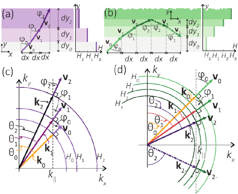
Figure 1: Schematic representation of the gradual bending of obliquely incident SW onto the region with increased [(a), (c)], and decreased [(b), (d)] value of the external magnetic field $H$. The alternate iso-frequency contours in (c) and (d) correspond to the alternate regions of decreasing and increasing values of the internal magnetic field $H_{i}$ in (a) and (b), respectively. The wave vectors $\textbf{k}_{i}$, vectors of the group velocities $\textbf{v}_{i}$, and their angles with respect to the $y$-axis, $\theta_{i}$ and $\varphi_{i}$, respectively, are indicated for each magnetic field segment $i$. The vertical dashed lines in (c) and (d) mark the conservation of the tangential component of the wave vector $k_{\|}$ at successive refractions and reflection. The insets on the right side of (a) and (b) correspond to $H$ values in accordingly marked regions.

II.2 Ray optic approximation

Let us analyze SWs propagation in a medium with slow, but a stepwise change of the internal magnetic field value along the $y$-axis from $H_{0}$, as shown schematically in the insets in Fig. 1 (a) and (b). We assume, that the dispersion relation obtained for a uniform thin film magnetized by the homogeneous in space external magnetic field (Eq. 2) can be used in each segment $i$ of the constant magnetic field $H_{i}$. SW ray propagating through an area with a gradual change of the internal magnetic field will be gradually bent due to the change of the magnetic field resulting in the variation of the SWs refractive index [see Fig. 1 (c) and (d)].

The bending of SW ray can be estimated from the conservation of the tangential to the interface component of the wave vector $k_{\|}$, $k_{i,\|}=k_{i+1,\|}$ Stigloher et al. (2016). As the interface, we refer to the $xz$ planes being perpendicular to the gradient of the magnetic field, which separates two successive segments with different magnetic fields, $H_{i}$, and $H_{i+1}$. Schematically it is shown in Fig. 1(c) and (d). To model SW beam propagation we will consider SW ray which can be treated as a curve on which are laying centroids of the SW beam. Rays follow the changes of the SWs group velocity direction ($\mathbf{v}_{i}$) as it is shown in Fig. 1(a) and (b) where $H$ increases and decreases along the $y$-axis, respectively. If we mark the angle of SW beam propagation by $\varphi$ (the angle of ($\mathbf{v}_{i}$) with respect to the $y$-axis) we can write

$$dy=\cot\varphi(y)dx,$$ (5)

and the function defining SW ray path $y\left(x\right)$ can be expressed in the recursive form:

$$y_{N}=y_{N-1}+\cot\varphi\left(y_{N-1}\right)dx$$ (6)

where $y_{N}=y\left(x_{N}\right)$, $x_{N}=x_{0}+Ndx$ and SW starts propagation from the point $\left(x_{0},y_{0}\right)$ with the angle of incidence $\varphi_{0}\equiv\varphi(y_{0})$. The direction of propagation, $\varphi$, is related to the direction of the energy transfer, i.e., the direction of the group velocity vector ($\mathbf{v}_{\mathrm{g}}=\nabla_{\mathbf{k}}\omega(\mathbf{k})$, where $\omega(\mathbf{k})=\omega(k_{x},k_{y})$ is a dispersion relation). The group velocity is normal to the iso-frequency contours. In the case of isotropic dispersion (considered in the paper), the iso-frequency contours are circular and the direction of the group and phase velocities are equal $\varphi=\theta$ where $\theta=\cot^{-1}k_{y}/k_{x}$. The angle of incidence can be expressed as

$$\cot\varphi(k_{x},k_{y})=\frac{v_{\mathrm{g},y}}{v_{\mathrm{g},x}}=\frac{\frac{\partial}{\partial k_{y}}\omega\left(k_{x},k_{y}\right)}{\frac{\partial}{\partial k_{x}}\omega\left(k_{x},k_{y}\right)}$$ (7)

where $v_{\mathrm{g},n}$ is $n$-th component of the group velocity. The initial conditions for the incident SW are known, hence a value of $k_{x}$ and angular frequency, $\omega$ at the starting point of SW are known. The normal component of the wavevector $k_{y}\left(\omega,H\right)$, can be calculated from Eq. (2) numerically or analytically. Exemplary iso-frequency contours lines for different values of the internal magnetic field $H_{i}$ with marked directions of group velocities corresponding to the fixed value $k_{\|}$ are shown in Fig. 1 (c) and (d).

Apart from refraction at the interface, there is possible also reflection. If the variation of the magnetic field between successive segments is small, most of the SW energy is transmitted (in the analytical model transmission is considered only), unless total reflection condition is fulfilled. In total reflection, there are no available solutions corresponding to the given $k_{\|}$ of the incident wave at some value of the internal magnetic field, e.g., in Fig. 1 (d) $|\textbf{k}_{3}|<k_{2,\|}$. In such a case SW is reflected from the interface, see Fig. 1(b) and (d) where such a situation is presented at the interface between $H_{2}$ and $H_{3}$. According to the law of reflection $\theta_{\mathrm{inc}}=\theta_{\mathrm{ref}}$ and $k_{y,\mathrm{ref}}=-k_{y,\mathrm{inc}}$, where superscripts “inc” and “ref” refer to the incident and reflected waves, respectively. Taking into account both, the bending and reflection of SWs, we can predict the SWs ray path for the conserved tangential component of the wavevector to the interface (aligned along the $x$-axis, $k_{x}=\mathrm{const.}$) using the following procedure:

$$dy=\begin{cases}\cot\varphi(y)dx&\mathrm{if\,}k\left(\omega,H\left(y\right)\right)\geq k_{x}\\ -\cot\varphi(y-dy)dx&\mathrm{if\,}k\left(\omega,H\left(y\right)\right)<k_{x}.\end{cases}$$ (8)

A similar model of the SWs propagation in a medium with a gradual change of the $\mathbf{H}$ caused by the demagnetizing field induced in the vicinity of the film’s edge was presented in Ref. Gruszecki et al. (2015). However, that model was valid only for isotropic SWs dispersion. This limitation is removed here due to the analysis of the group velocity direction instead of the wave vector.

II.3 Micromagnetic simulations

Micromagnetic simulations have been proven to be an efficient tool for the calculation of SW dynamics in ferromagnetic materials. Presented results were obtained using the MuMax3 Vansteenkiste et al. (2014) which solves time-dependent LLG equation (1) with included Landau damping term with the finite difference method. In simulations, we consider an oblique SW beam propagation in YIG thin film saturated by an OOP magnetic field. We assume typical magnetic parameters of YIG at 0K, it is $A=0.4\times 10^{-11}$ J/m, $M_{\mathrm{S}}=0.194\times 10^{6}$ A/m, $\gamma=176$ rad GHz/T and the value of damping $\alpha=0.0005$. The system of size $L_{x}\times L_{y}\times L_{z}$ was discretized with cuboid elements of dimensions $l_{x}\times l_{y}\times L_{z}$. Lateral dimensions of the single cell $l_{x}\times l_{y}$ and film thickness $L_{z}=10$ nm are less than the exchange length of YIG, $13$ nm. The simulations have been performed for two geometries: i) 6 $\mu$m $\times$ 4 $\mu$m $\times$ 10 nm discretized with the cell of lateral dimensions $2\times 2$ nm² for high-frequency exchange SWs and ii) 32 $\mu$m$\times$4 $\mu$m$\times$10 nm discretized with the cell of size $8\times 8$ nm² for SWs of lower frequency (15 GHz).

Every simulation comprises two parts. First, we get the equilibrium static magnetic configuration, which in our study is always OOP magnetization. Then, the results of the first stage are used in the dynamic part of simulations, which are aimed at obtaining the steady-state. SWs are continuously generated in the form of a Gaussian beam which propagates through the film. At the edges of the film $x=0$ and $x=L_{x}$, absorbing boundary conditions are applied . SW beams are excited by means of the spatially non-uniform dynamic external magnetic field at a given frequency and the spatial profile designed to excite the SW beam of appropriate width. The profile of the dynamic magnetic field used to excite the SW beam is similar to the profile generated by a coplanar waveguide with modulated width Gruszecki et al. (2016) multiplied by the Gaussian function changing its value along the axis of the coplanar waveguide. The exact description of the SWs’ beam excitation can be found in Ref. Gruszecki et al. (2017). After sufficiently long time of continuous excitation, when the beam is clearly visible and doesn’t change qualitatively in time, a steady-state is achieved. The data necessary for further analysis are stored. From the stored micromagnetic simulations results rays corresponding to the excited SW beam are extracted. Firstly, the time average SW intensity colormaps are obtained for simulation according to the equation: $I(x,y)=\frac{f}{4}\int_{0}^{4/f}\left[m_{x}\left(x,y,t\right)\right]^{2}dt$, where $m_{x}$ is normalized component of the magnetization vector. Then, the Gaussian fitting is applied to get ray line coordinates (details can be found in Ref. Gruszecki et al. (2014)). Those ray lines are directly compared with the results of the analytical model.

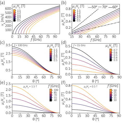
Figure 2: (a) The group velocity of SWs in the OOP magnetized YIG film of thickness 10 nm in dependence on frequency, plotted for several values of the homogeneous, static external magnetic field, $H_{0}$. (b) Critical external magnetic field $H_{\mathrm{cr}}$ in dependence on SWs frequency for the angle of incidence 60° and several values of the external magnetic field (solid lines), and also for $\mu_{0}H_{0}=0.5$ T and the angle of incidence 50° (black dash-dotted line), and 70° (black dashed line). $H_{\mathrm{cr}}$ in dependence on the angle of incidence and several values of $H_{0}$ for SWs of frequency, in (c) for 100 GHz and in (d) for 15 GHz. $H_{\mathrm{cr}}$ in dependence on the angle of incidence and several values of SWs frequency for (e) $\mu_{0}H_{0}=1.5$ T and (f) $\mu_{0}H_{0}=0.5$ T.

III Results

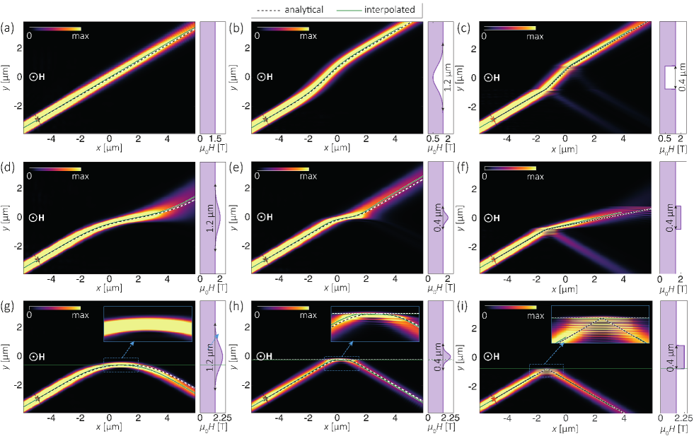
Figure 3: The micromagnetic simulations results presenting SWs intensity maps obtained for SW beams of frequency $f=100$ GHz incident under the angle $\theta=60$° in the $10$ nm thick YIG film. Solid green lines and dashed black lines correspond to the results interpolated from simulations and calculated using the analytical model, respectively. The static magnetic field (directed OOP) depends only on the $y$ coordinate. Its profile is presented in the insets on the right side of each figure. In (g)-(i), the horizontal overlapping lines correspond to the plane of reflection and their positions obtained from the analytical model and extracted from micromagnetic simulations perfectly agree. The insets in right top corners of (h) and (i) present zoomed in regions of the simulated area marked via dashed green rectangle. (a) SW beam propagation in the medium with uniform $H$; incline SW beam propagation through the region with the (b) gradual and (c) step decrease of the magnetic field. (d) and (e) gradually increased $H$ value up to 2.0 T at $y=0$ with a different gradient of $H$ changes; (f) step-index change of $H$ up to 2.0 T in the central region of the film. (g) and (h) gradually increased $H$ value up to 2.25 T for $y=0$ with different profiles of $H$; (i) step-index change of $H$ up to 2.25 T in the central region of the film. In (d)-(e) SW beam is spread due to small field increase, this $H$ modulation effectively works as an diverging lens; in (e) the small part of SW beam energy is also reflected; in (f) a part of the energy is reflected at both first and second interface. In (g)-(i) the total internal reflection of SW beam is visible. (g) The total internal reflections at the region with the gradually changing refractive index is referred to as a mirage. In (h) is visible a large shift between the incident and reflected beam spots, at some range, SW beam propagates parallel to the interface.

III.1 Analytical model

In OOP magnetized thin film the SW ray angle with respect to the $y$-axis is given by

$$\cot\varphi(y)=\cot\theta(y)=\frac{k_{y}}{k_{x}}=\frac{\sqrt{k^{2}\left(\omega,H\left(y\right)\right)-k_{x}^{2}}}{k_{x}},$$ (9)

where the value of $k\left(\omega,H\left(y\right)\right)$ can be calculated numerically from the dispersion relation Eq. (2). The results of the analytical analysis of the SW rays are shown in Fig. 1(a) and (b) for the increased and decreased internal magnetic field, respectively.

The knowledge about the group velocity of SWs during their propagation through the film is important from an application point of view. Exemplary results showing how $v_{\mathrm{g}}$ depends on the SWs frequency for different values of the external magnetic field are presented in Fig. 2(a). It is shown, that $v_{\mathrm{g}}$ for OOP configuration monotonously increases (apart from the region of dominating magnetostatic interactions at low frequencies, invisible in the figure)Stancil and Prabhakar (2009) with an increase of the frequency and decrease of the external magnetic field value. Therefore, SWs falling at a region with decreased $H$, and thus the increased refractive index, accelerates. That situation is opposite to optics, where an increase of the refractive index is related to a decrease of the group velocity of electromagnetic waves.

The effect of total internal reflection is important for wave applications, especially in designing of the waveguides. We will analyze the total internal reflection of SWs in the OOP magnetized film with spatially modulated magnitude of the static external magnetic field $H(y)=H_{0}+H^{\prime}(y)$, where $H^{\prime}(y)$ is its modulation, which in the case under investigation, depends only on the $y$ coordinate. Therefore, we will analyze the critical field $H_{\mathrm{cr}}$ at which the total internal reflection takes place in dependence on frequency, $H_{0}$, and the angle of incidence. The results for $\mu_{0}H_{0}=$ 0.5-1.5 T with an interval 0.2 T and $\varphi=60\text{\textdegree}$, and additionally, for angles of incidence 50° and 70° at $\mu_{0}H_{0}=0.5$ T are shown in Fig. 2(b). It is visible that with the increase of $\varphi$ the smaller value of the field $H_{\mathrm{cr}}$ is required to obtain total internal reflection. Furthermore, the greater $\varphi$ the smaller slope of $H_{\mathrm{cr}}\left(f\right)$, and interestingly, these dependencies are linear.

The dependencies of $H_{\mathrm{cr}}$ on the angle of incidence for different values of $H_{0}$ and $f$ are in details presented in Fig. 2(c)-(f). In Fig. 2(c) and (d) are dependencies of $H_{\mathrm{cr}}$ on the angle of incidence for SWs at frequencies 100 GHz and 15 GHz, respectively, and for different values of $H_{0}$. It is visible, that while the angle of incidence increases, the value of $H_{\mathrm{cr}}$ decreases. Moreover, the higher value of $H_{0}$ the smaller $H_{\mathrm{cr}}$ is needed to obtain total internal reflection. It is, because, while $H$ increases the FMR (ferromagnetic resonance) frequency increases as well. Therefore, the greater length of wavevector (frequency is much higher than the FMR frequency) the higher value of $H_{\mathrm{cr}}$ is required to obtain total internal reflection. In Fig. 2(e) and (f) are presented dependencies of $H_{\mathrm{cr}}$ on the angle of incidence for $\mu_{0}H_{0}=$ 1.5 and 0.5 T, respectively, for different values of $f$. It is shown, that the higher frequency, the larger modulation of $H^{\prime}(y)$ is needed to obtain total internal reflection, what is consistent with previous analysis.

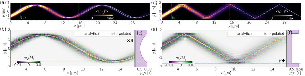
Figure 4: Spin-wave beam propagating under the angle of 60° at frequency $f=15$ GHz in $10$ nm thick and 4 $\mu$m wide YIG stripe in presence of gradual (a)-(c) and step (d)-(f) changes of the external magnetic field across the stripe’s widths. The respective profiles of the magnetic field across the stripe are shown in (c) and (f). In (a) and (d) the SWs intensity obtained from micromagnetic simulations is shown; in (b) and (e) the amplitude of SWs from the fragment of the structures presented in (a) and (d) (marked by the green rectangle with dashed sides), respectively, are plotted. The dashed red lines show the result of the ray model which match well with the ray extracted from micromagnetic simulations, marked with the solid-yellow lines.

III.2 Micromagnetic simulations

The predictions of the analytical model we validated by means of micromagnetic simulations. Those simulations were performed for i) high-frequency $f=100$ GHz exchange dominated SWs and ii) lower frequency SWs, $f=15$ GHz.

In Fig. 3 we show the SW intensity maps (the square of the dynamic component of the magnetization averaged over time: $\left\langle m_{x}^{2}\left(x,y,t\right)\right\rangle_{1/f}$). The results are presented for the exchange dominated SW beams of the beam width c.a. 700 nm and wavelength 33.6 nm (at 100 GHz) incident under the angle 60° at the region with varied magnetic field $H\left(y\right)=H_{0}+H^{\prime}\left(y\right)$, where $\mu_{0}H_{0}=1.5$ T and $H^{\prime}\left(y\right)$ is a Gaussian function. Additionally, we show SW rays obtained from the analytical model (black-dashed lines) from Eq. (8) and extracted from the MS results (green-solid line) for different profiles of $H^{\prime}\left(y\right)$ in (a)-(i). Overall, the very good agreement between micromagnetic simulations and the analytical model is found.

Accordingly with the model predictions in Fig. 1(a) the decrease of $H$ results in the gradual decrease of the angle of refraction, see Fig. 3(b) and (c). It causes the shift of the transmitted beam along the $x$-axis with respect to the case of unbent SW beam [Fig. 3(a)]. In the case of gradually decreasing $H\left(y\right)$ the SW beam reflections from the nonuniform region are not visible [Fig. 3(b)], whereas in the case of step-index change of $H\left(y\right)$ the reflected SW beams are apparent [Fig. 3(c)]. In the case of step-index change of $H\left(y\right)$, the interference pattern of the incident and reflected waves is visible as horizontal stripes with higher and lower intensities near the interface.

The increase of $H(y)$ causes the increase of the angle of refraction [Fig. 3(d)-(i)], which is also according to the model estimation shown in Fig. 1(a). When the increase of the magnetic field is slow and the maximal value of $H\left(y\right)$ is smaller than $H_{0}+H_{\mathrm{cr}}$, the refracted SW beam is spread, see Fig. 3(d). Hence, that region with increased $H$ can be treated as a diverging lens for SWs in analogy to optics Hecht (1998). For more abrupt changes of $H\left(y\right)$, clearly visible reflected SW beams appears [Fig. 3(e)]. In the limit of the step-index change of $H\left(y\right)$ the incident SW beam is split into transmitted and pronounced reflected SW beams, see Fig. 3(f).

For higher maximal values of the external magnetic field, exceeding the condition for total internal reflection $\max\left(H\left(y\right)\right)>H_{0}+H_{\mathrm{cr}}$, the incident beam is totally reflected [Fig. 3(g)-(i)]. It is noteworthy that the magnetic field at which the total internal reflection takes place is almost identical in the case of micromagnetic simulations and analytical model, see two overlapping horizontal dashed lines in Fig. 3(g)-(i). These horizontal lines correspond to the value of the external magnetic field $H=H_{0}+H_{\mathrm{cr}}$ and can be referred to as the interface at which total internal reflection takes place. Interestingly, for the slow increase of $H(y)$, the equivalent of the mirage effect for SWs is apparent [see Fig. 3(g)]. It means, that the wavefronts of incident SW beam are gradually bent without reflection, and the interference pattern near the interface is not visible.

For the rapid change of the $H(y)$ magnitude, the interference pattern near the area of the varied magnetic field is present, pointing at the reflection of waves. In this scenario, the SW ray near the interface becomes almost parallel to its line for some distance, see Fig. 3(h). It means, that between the incident and reflected SW beam spots appears lateral shift along the interface of value almost 1 $\mu$m. One may call this phenomenon as Goos-Hanchen effect for SWs Gruszecki et al. (2014); Goos and Hänchen (1947) of surprisingly high value. However, we fully recreated this effect using ray optics approximation only (see the dashed black line), whereas the literature Goos-Hanchen effect is a wave phenomenon, defined as a lateral shift between the incident and reflected beam spots due to phase change occurring at the interface Artmann (1948). It means, the Goos-Hanchen effect cannot be explained by the use of ray optics approximation, therefore, the observed lateral shift shouldn’t be referred to as the Goos-Hanchen shift, although, the observed phenomenon looks equivalently in the far field. For the step change of $H(y)$ [Fig. 3(i)], neither lateral shift nor bending are visible. The interference pattern is clearly apparent and there is no transmission to the upper part of the sample.

In the last part of our study, we verify analytical predictions for lower frequency SWs and the ferromagnetic stripe of the finite width. We analyze the SW beam at the frequency $f=15$ GHz (wavelength 115 nm) with the beam width 680 nm propagating in the 10 nm thick and 4 $\mu$m wide YIG stripe OOP magnetized by the external magnetic field. The value of $H(y)$ in the middle part is set as $\mu_{0}H_{0}=0.5$ T and its magnitude gradually increases when moving to the stripe edges up to $\mu_{0}H\left(w\right)=0.58$ T near the sides of the stripe, at a distance $w=1.6$ $\mu$m from the center of the stripe [see Fig. 4(c)]. The quadratic change of the field $H\left(y\right)=H_{0}+H_{\mathrm{m}}^{\prime}y^{2}/w^{2}$, where $\mu_{0}H_{\mathrm{m}}^{\prime}=0.08$ T, is assumed.

In Fig. 4(a) the SW beam propagates under the angle 60° with respect to the $y$-axis counted in the middle part of stripe and is multiple times reflected in the considered part of the waveguide. Under the assumption of the realistic value of the damping in YIG, the SW beam propagates for a distance up to 30 $\mu$m with reasonable intensity. The bending of the wavefronts in the region with the gradually increased magnetic field is demonstrated in Fig. 4(b), which is similar to the observation made in Fig. 3(g) for high-frequency SWs. The ray of the propagating SW beam obtained from the analytical model, Eq. (8), is shown with the red dashed line. The satisfactory agreement between analytical and simulation results is found at the beginning part of the waveguide, but this negligible discrepancy, increases with a distance, pointing out that wave effects, which are not taken into account in the ray model, exist in the propagation through GI media, and accumulate with a distance.

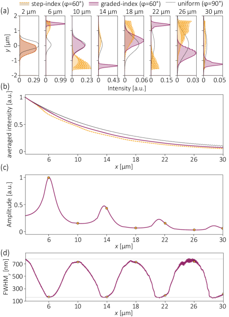
Figure 5: (a) Spin-wave beam profile across the width of stripe presented in Fig. 4 for several values of $x$. Solid violet and dashed yellow lines have been obtained for the SW beam profiles excited with $\varphi=60^{\circ}$ and propagating in the GI and the step index stripes, respectively. The thin black dashed line corresponds to the SW beam of the same width but propagating along the $x$-axis ($\varphi=90^{\circ})$ in the uniform magnetic field. The SWs intensity is normalized to the maximal intensity in the whole waveguide for all simulations. (b) The averaged intensity of SWs across the stripe’s width as the function of $x$ for two different profiles of the external magnetic field: step-index (dash-dotted magenta line), and GI (dashed yellow line). These results are compared with SW beam propagating along the $x$-axis in the uniformly magnetized stripe. (c) Maximal amplitude of the SW beam in GI stripe in dependence on $x$. (d) SW beam’s width (full width at half maximum) evolution in the GI stripe in dependence on the $x$ coordinate. Golden dots in (c) and (d) correspond to the profiles of SW beam in GI stripe presented in (a).

For a comparison, micromagnetic simulations have been performed for the step-index change of $H\left(y\right)$ at $y=\pm w$, see the field profile in Fig. 4(f). The SW beam in such a system [see Fig. 4(d) and (e)] can propagate in the form of the narrow beam for a shorter distance, than in the GI waveguide. The additional simulation has been performed also for the SW beam of the same profile in the beam waist propagating along the $x$-axis ($\varphi=90^{\circ}$) in the waveguide saturated by the uniform external magnetic field of value $\mu_{0}H_{0}=0.5$ T. The results of simulations are presented in Fig. 5(a), where profiles of intensities of SW beams propagating in above described three waveguides (with GI, step-index and constant profile of the magnetic field) at eight different distances along the $x$-axis are shown. It is clear that the SW beam propagating in the GI waveguide preserves its width for a much longer distance than other two waveguides. For instance, at $x=26$ $\mu$m the SW beam width is comparable with that at $x=2$ $\mu$m, whereas for step-index waveguide SW beam is spread across the whole width of the waveguide. Interestingly, the SW beam in GI waveguide is much narrower, than the input beam, in the areas where the total internal reflection occurs (see profile for $x=6$ $\mu$m).

Furthermore, we analyze the change of the averaged intensity of SW beams along the waveguide’s width with increasing $x$ for different $H\left(y\right)$ profiles, see Fig. 5 (b). For all profiles of $H\left(y\right)$ the dependencies are similar because it is due to damping constant $\alpha$ in Eq. 1. One can observe, that decay of the SW beam amplitde excited with $\varphi=90^{\circ}$ is slightly slower than for beams excited with $\varphi=60^{\circ}$ in the GI and step-index waveguides. However, the difference results from different optical paths of the beams in the analyzed examples, i.e., the shortest path is obtained for the SW beam excited with $\varphi=90^{\circ}$ in a waveguide magnetized by the uniform field $H(y)=H_{0}$, and the longest for the SW beam excited with $\varphi=60^{\circ}$ propagating in the step-index fiber. SW beam propagating in the GI waveguide, due to its bending, possess the moderate effective length of the beam ray.

Finally, we analyze in details SW beam behavior in GI waveguide. In Fig. 5(c) and (d) the SW beam amplitude and the full width at half maximum (FWHM_y) taken along the $y$-axis, respectively, are plotted in dependence on $x$. The local maxima in Fig. 5(c) correspond to the SWs beam narrowing while it propagates near the waveguide edges. In the region near the critical value of $H$ SWs intensity is around 3 times larger than in the central part of the waveguide. Therefore, the more pronounced maxima, the more collimated SW beam is. This is confirmed by the FWHM${}_{y}\left(x\right)$, which oscillates between its maximal width (located near the center of the waveguide, FWHM${}_{y}=780$ nm) and the minimal width (located near the critical value of the $H$, FWHM${}_{y}=160$ nm). Any systematic beam’s spreading along the $x$ is visible and the ratio between maximal and minimal widths is kept being equal 4. Overall, it means that the stripe with GI modulation of $H\left(y\right)$ preserves the best transmission properties from all analyzed cases.

The significant difference in SW beam propagation between the stripe with the gradual and step change of the static magnetic field, proofs that the stripes with graded refractive index are promising candidates for transmitting signals carried by SWs. The system under investigation can be referred to as a wide, multimode GI waveguide for SWs. We believe the proposed system can be a good playground to study SW beam guiding and can be directly used for an experimental demonstration of the investigated effects, e.g., using recently experimentally validated in Ref. Körner et al. (2017) method of SW beams excitation.

IV Summary

We have studied SW beam propagation in the ferromagnetic film and waveguide with a gradual change of the magnetic field. These structures can be referred to as magnonic GI media, for which non-uniformity of the refractive index is introduced by the variation of the external magnetic field magnitude. For the sake of simplicity, we performed all investigations for the out-of-plane magnetized thin YIG films. Nevertheless, the study can be extended into other materials and other magnetic configurations. We have proposed the ray optic approximation to describe SW beam propagation through an area of the ferromagnetic film with the gradual variation of the magnetic field value. We have successfully verified the analytical model by micromagnetic simulations for high and relatively low-frequency SWs in an exchange regime, for which the magnetostatic effects are negligible. We have demonstrated bending of the SW beam propagating obliquely through regions with GI, the total internal reflection, and the mirage effect with narrowing of the SW beam. We have also demonstrated that a region with the inhomogeneous magnetic field value can be used to obtain a diverging SW lens. Thin ferromagnetic stripe with an inhomogeneous magnetic field across its width has been used to study GI materials for SW guiding. The obtained results have been compared with results for the stripe with a step-index change of the external magnetic field. We show, that the stripe with the gradual modulation of the SW refractive index possesses better transmission properties than the step-index stripe. Interestingly, SW beam propagating in the GI stripe is periodically narrowed in the region of the reflection at areas with the internal field fulfilling the condition for total internal reflection, and then again spreads. Ultimately, any systematic beam spreading has not been observed for stripe with GI, as opposed to the step-index stripe, or SW beam propagating along the stripes axis. It points out, that this approach can be used to transmit SW beam without beam widening for very long distances, limited only by damping. We believe, that the use of SWs waveguides with additional GI cladding shall significantly reduce the influence of defects at the edges of the ferromagnetic stripes, reduce spreading of the SW beam width, and enhance the transmission. Further investigations are necessary for the optimization of the multi- and single-mode SW waveguides, and for other magnetization configurations.