Expelled grains from an unseen parent body around AU Mic

Abstract

Context. Recent observations of the edge-on debris disk of AU Mic have revealed asymmetric, fast outward-moving arch-like structures above the disk midplane. Although asymmetries are frequent in debris disks, no model can readily explain the characteristics of these features.

Aims. We present a model aiming to reproduce the dynamics of these structures, more specifically their high projected speeds and their apparent position. We test the hypothesis of dust emitted by a point source and then expelled from the system by the strong stellar wind of this young, M-type star. In this model, we make the assumption that the dust grains follow the same dynamics as the structures, i.e. they are not local density enhancements.

Methods. We perform numerical simulations of test particle trajectories to explore the available parameter space, in particular the radial location $R_{0}$ of the dust producing parent body and the size of the dust grains as parameterized by the value of $\beta$ (ratio of stellar wind and radiation pressure forces over gravitation). We consider both the case of a static and an orbiting parent body.

Results. We find that, for all considered scenarii (static or moving parent body), there is always a set of ($R_{0},\beta$) parameters able to fit the observed features. The common characteristics of these solutions is that they all require a high value of $\beta$, of around 6. This means that the star is probably very active and the grains composing the structures are sub-micronic, in order for observable grains to reach such high $\beta$ values. As for the location of the hypothetical parent body, we find it to be closer-in than the planetesimal belt, around $8\pm 2$ au (orbiting case) or $28\pm 7$ au (static case). A nearly periodic process of dust emission appears, of 2 years in the orbiting scenarii, and 7 years in the static case.

Conclusions. We show that the scenario of sequential dust releases by an unseen, point-source parent body is able to explain the radial behaviour of the observed structures. We predict the evolution of the structures to help future observations to discriminate between the different parent body configurations that have been considered. In the orbiting parent body scenario, we expect new structures to appear on the northwest side of the disk in the coming years.

1 Introduction

AU Mic is an active M-type star, in the $\beta$ Pictoris moving group, with an age of 23 $\pm$ 3 Myr (Mamajek & Bell 2014). Its debris disk, seen almost edge-on, has been imaged for the first time by Kalas et al. (2004) in the optical. The dust seen in scattered light has been shown to originate from collisional grinding of planetesimals arranged in a belt at $\sim$35-40 au (Augereau & Beust 2006; Strubbe & Chiang 2006; Schüppler et al. 2015). The belt was later resolved by millimeter imaging (Wilner et al. 2012; MacGregor et al. 2013). Because the star is very active, the dynamics of the dust grains is believed to be strongly affected by the stellar wind.

Recently, Boccaletti et al. (2015) have revealed five fast-moving, arch-like, vertical features in this disk in scattered light imaging with HST/STIS (Schneider et al. 2014) and VLT/SPHERE (Beuzit et al. 2008) at three different epochs. The five structures, named A to E, are shown in Figure 1. They are identified in the 2010, 2011 and 2014 images, except for the A structure which was too close to the star in 2010. Curiously, these structures are all located on one single side of the disk and they all show an outward migration. For the D and E structures, the velocities are such that these features could match asymmetries identified in earlier, multiple wavelength observations (Liu 2004; Krist et al. 2005; Metchev et al. 2005; Fitzgerald et al. 2007). Although they move outward, the arch-like structures seem stable in shape over a time span of a few years.

Figure 1: 2010 and 2011 HST/STIS and 2014 VLT/SPHERE images of the debris disk of AU Mic. The five structures are identified in the bottom panel.

The projected speeds derived from the observations are displayed in Figure 2. One can see that they increase with rising distance to the star. The two outermost, at least, are exceeding the local escape velocity. There is currently no theorical framework to readily explain this behaviour (see e.g. Matthews et al. 2014, for a recent review on debris disks). Any dynamical process involving copious amount of gas, such as radiation-driven disk winds which may allow to reach high velocities are excluded by the low amount of gas remaining around AU Mic (Roberge et al. 2005 fixed an upper limit of H₂ mass at 0.07 $M_{\oplus}$). Vertical resonances with a planetary companion can form arch-like structures, but they stay on a Keplerian orbit (analogous to the case of Saturn’s moons, see e.g. Weiss et al. 2009). Lindblad resonances can induce spiral density arms phase-locked with a perturber, but if each structure corresponds to an arm, they would be observed on both sides of the disk. Concentric eccentric rings resulting from massive collisions of asteroid-like objects can produce local intensity maxima (e.g. Kral et al. 2015), but this process requires a time scale of 100 years, while the structures escape the system in tens of years.

Figure 2: Apparent speeds of the structures in the AU Mic debris disk derived from the observations (Tabs. 2 and 5). The gray region shows the escape velocities for stellar masses ranging from 0.3 to 0.6 M_⊙, the dotted line corresponding to a mass of 0.4 M_⊙.

In this study, we aim to reproduce the observed high speeds and apparent positions of the structures. We leave aside in this paper the origin of the vertical elevation of the structures. In Section 2 we describe our model. There, we assume that the NW/SE asymmetry can be explained by a local process of dust release. This hypothetic emission source will be refered to as parent body in the following, without further specification. Boccaletti et al. (2015) , for instance, proposed that this could correspond to a planet, which magnetosphere or dust circumplanetary ring would be interacting with the stellar wind. The dust released by the parent body is exposed to the stellar wind. The resulting wind pressure can put this dust on unbound trajectories, achieving the observed high projected speeds. In Section 3, we explore the case of a static parent body, that would for example mimic a source of dust due to a giant collision (e.g. Jackson et al. 2014; Kral et al. 2015) or a localised dust avalanche (Chiang & Fung 2017), and the case of an orbiting parent body, for example, a young planet. However, we emphasize that we do not suppose any specific dust production process in our study. Instead, we focus on the dynamical evolution of the dust right after its release, and any dust production mechanism will have to comply with the constraints we derive on the dust properties and dynamics. We discuss our findings, the influence of the parameters, and the implications in Section 4.

2 Model

We develop a model that aims to investigate the dynamics of dust particles released by a singular parent body and affected by a strong stellar wind pressure force. Throughout this paper, we make the important assumption that the observed displacements correspond to the actual proper motion of the particles, and not to a wave pattern, which implies that the particles are supposed to have the same projected speeds as the observed structures. We seek to discuss if this assumption could yield to scenarii that allow to reproduce the observed speeds in the AU Mic debris disk, and which conditions must be fulfilled.

2.1 Parent body

To break the symmetry of the disk, we need an asymmetric process of dust production. The dust arranged in the fast-moving structures is thus assumed to be locally released by an unresolved, unknown source: the ”parent body”. This hypothetical parent body will not be described further, but we note that it must be massive enough to produce a significant amount of dust, although it should remain faint enough to be undetected with current instrumentation. Actually, the upper mass limit is fixed by the non detection of point source in SPHERE imaging. This implies a compact parent body smaller than 6 Jupiter masses beyond 10 au (see Methods of Boccaletti et al. 2015). The process of dust production is neither described in this model, except that it must be sporadic otherwise we would observe one single, continuous feature. We can thus exclude the flares of the star for being the trigger events responsible for the arch formation as they are too frequent (0.9 flare per hour following Kunkel 1973).

The parent body is assumed to be at a distance $R_{0}$ from the star in the plane of the main disk. When supposed to be revolving around the star, its orbit is considered to be circular. The dust particles are released with the local Keplerian speed.

2.2 Pressure forces

Figure 3: $\beta$ values as a function of grain size. The material used for $\beta_{\mathrm{PR}}$ is M1 of Schüppler et al. (2015). Two hypothesis for the mass-loss rate of the star are shown (solid and dashed lines). The horizontal solid black line is the upper limit for bound trajectories assuming zero eccentricity for the parent body, and the dashed line is the limit between ”normal” and ”abnormal” parabolic trajectories (see Sec. 2.3).

Supposing that the observed velocities correspond to the effective speeds of the particles, that means they accelerate outwards once released, to finally exceed the escape velocity. As the particle size decreases, they are more affected by the pressure coming from the stellar wind. The radiation pressure is also more efficient although it remains low because AU Mic is an M-type star. These processes can accelerate outward the particles, provided the total pressure force exceeds the gravitational force.

The two pressure forces will be described by a single parameter noted $\beta$ in the following. It is the ratio of the wind plus radiation forces to the gravitational force

$$\beta=\frac{||\mathbf{F}_{\rm SW}||+||\mathbf{F}_{\rm PR}||}{||\mathbf{F}_{\rm grav}||}=\beta_{\rm SW}+\beta_{\rm PR},$$ (1)

under the assumption that the grain velocity $v$ is such that $v\ll c$ and $v\ll V_{\rm sw}$ where $c$ is the light speed in vacuum and $V_{\mathrm{sw}}$ is the wind speed. $\mathbf{F}_{\rm SW}$ is the force exerted by the stellar wind on the particle. $\mathbf{F}_{\rm PR}$ is the radiation force, taking into account the radiation pressure and the Poynting-Robertson drag. $\mathbf{F}_{\rm grav}$ is the gravitational force of the star. For typical silicate submicrometer-sized grains, $\beta$ ranges from $\sim 10^{-1}$ to a few tens (see Fig. 1 of Schüppler et al. 2015 and Fig. 11 of Augereau & Beust 2006).

The two contributions to $\beta$ can be estimated with, for example, Eq. 28 of Augereau & Beust (2006) and Eq. 6 of Strubbe & Chiang (2006), respectively:

$$\beta_{\rm SW} = \frac{3}{32\pi}\frac{\dot{M}_{\star}V_{\mathrm{sw}}C_{\mathrm{D}}}{GM_{\star}\rho s},$$ (2)

$$\beta_{\rm PR} = \frac{3}{16\pi}\frac{L_{\star}\langle Q_{\mathrm{PR}}\rangle}{c\,GM_{\star}\rho s},\mathrm{\,\,\,with\,\,\,}\langle Q_{\mathrm{PR}}\rangle=\dfrac{\int_{\lambda}F_{\lambda}Q_{\mathrm{PR}}\mathrm{d}\lambda}{\int_{\lambda}F_{\lambda}\mathrm{d}\lambda},$$ (3)

where $\dot{M}_{\star}$ is the stellar mass loss rate, $C_{\mathrm{D}}$ the dimensionless free molecular drag coefficient which has a value close to 2, $G$ the gravitational constant, $M_{\star}$ the mass of the star, $\rho$ the grain volumetric mass density, $s$ the grain radius, $L_{\star}$ the stellar luminosity, $Q_{\mathrm{PR}}$ the dimensionless radiation pressure efficiency (that depends on the grain size, composition and wavelength), and $F_{\lambda}$ the stellar flux at wavelength $\lambda$.

$\beta_{\rm PR}$ is independent on the grain’s distance to the star ($r$), but $\beta_{\rm SW}$ can slightly depend on $r$ (e.g. Fig. 11 in Augereau & Beust 2006). In this study, we will neglect this effect. $\beta$ is highly size-dependent. For sufficiently large grains ($s\gtrsim 1\mu$m in the case of AU Mic), $\beta$ varies as $s^{-1}$ (Schüppler et al. 2015). For smaller grain sizes, the relationship between $\beta$ and $s$ is more complex (e.g. Fig. 1 in Schüppler et al. 2015) and depends both on the grain composition, the stellar mass loss rate $\dot{M}_{\star}$ and the stellar wind speed $V_{\mathrm{sw}}$. With $\dot{M}_{\star}=50\,\dot{M}_{\odot}$ and $V_{\mathrm{sw}}=V_{\mathrm{sw,\odot}}$, the blowout size (grains with $\beta=0.5$, assuming zero eccentricity for the parent body) is 0.04 $\mu$m (Fig. 3). This size jumps to 0.35 $\mu$m if the stellar mass-loss rate is increased to $300\,\dot{M}_{\odot}$. These values are consistent with those reported in Tab. 2 of Schüppler et al. (2015) although they slightly differ because of minor differences in the assumed stellar properties.

2.3 Particles behaviour

The trajectory of a grain released from a parent body strongly depends on the $\beta$ value. For a parent body on a circular orbit, the released $0<\beta<0.5$ dust particles remain on bound orbits, with eccentricities increasing with $\beta$, while the $0.5<\beta<1$ particles are placed on parabolic orbits. Dust particles with $\beta>1$ will, on the other hand, follow unbound, ”abnormal” parabolic trajectories, as described for example in Krivov et al. (2006). These $\beta>1$ grains are of particular interest in the context of the AU Mic debris disk because their velocity continuously increases while moving outwards, until it reaches an asymptotic value that can be evaluated by considering the total energy per unit of mass of the particle at a distance $r$ from the star:

$$e_{m}=\frac{1}{2}v^{2}-\frac{GM_{\star}}{r}(1-\beta),$$ (4)

where $M_{\star}(1-\beta)$ is the apparent mass of the star. The particle is supposed to be released with the Keplerian velocity $v_{0}=\sqrt{GM_{\star}/R_{0}}$ at radius $R_{0}$. Evaluating Eq. 4 in $R_{0}$ thus yields:

$$e_{m}=\frac{GM_{\star}}{2R_{0}}(2\beta-1)\,.$$ (5)

Therefore, the asymptotic speed reached by the dust particle far away from the star (valid for $\beta>0.5$) is given by:

$$v_{\infty}=v(r\rightarrow\infty)=\sqrt{(2\beta-1)\frac{GM_{\star}}{R_{0}}}=v_{0}\sqrt{2\beta-1}.$$ (6)

For the $0.5<\beta<1$ grains, $v_{\infty}$ is smaller than $v_{0}$. In this case, the asymptotic value of the velocity is reached by upper values and the speed decreases with the distance from the star. The $\beta\leavevmode\nobreak\ >\leavevmode\nobreak\ 1$ grains, on the other hand, reach the asymptotic value of the velocity by lower values, and $v$ increases with $r$. This behaviour is illustrated in Fig. 4. As shown in Fig. 2, the observed apparent speeds are not compatible with bound orbits at least for the structures D and E. An unbound orbit is equivalent to $\beta>0.5$ in the model. Furthermore, the global trend of increasing velocity with the distance to the star is only reproduced by trajectories with $\beta>1$ (see Fig. 4).

Figure 4: Module of the velocity as a function of the distance from the star for a particle released with the Keplerian speed at 8 au . The solid curves correspond to $\beta$=0.3 (blue), 0.7 (green), 1.5 (red) and 5.6 (cyan). The horizontal dashed lines are the asymptotic values of the velocity derived from Eq. 6.

Table 1: Documented stellar parameters of AU Microscopii (GJ803, HD~197481)

Parameter	Value	Reference
Spectral type	M1Ve	Torres et al. (2006)
Age	$23\pm 3$ Myr	Mamajek & Bell (2014)
Distance	9.94 $\pm$ 0.13 pc	Perryman et al. (1997)
Mass ($M_{\star}$)	0.3-0.6 M⊙	Schüppler et al. (2015)
Wind speed ($V_{\mathrm{sw}}$)	$4.5\times 10^{5}$ m/s	Strubbe & Chiang (2006)

The strength of the pressure forces on the grains, characterized by $\beta$, and the released position of the grains, $R_{0}$, are two key parameters in this model, and some constraints on their values and relationship can be anticipated. For instance, should the grains be on bound orbits ($\beta<0.5$), their apoastron $r_{a}=(1-2\beta)^{-1}R_{0}$ should be sufficiently large for the particles to reach the position of the furthest structures, around 50 au in projection (structure E). Noting $r_{E}$ the apparent position of the E structure, the condition $r_{a}\gtrsim r_{E}$ yields a strict lower limit on $\beta$:

$$\beta>\frac{r_{E}-R_{0}}{2r_{E}}.$$ (7)

Nevertheless, we anticipate unbound orbits with high $\beta$ values to best fit the observed speeds, and a power law linking $\beta$ and $R_{0}$ can be approximated analytically. The trajectories of grains with $\beta$ values much larger than 1 are almost radial and the limit speed reached by the particle is given by Eq. 6. The data points to reproduce are apparent speeds at projected distances. Let us take the pair ($r_{D},v_{D}$) for the D structure as an example, and note $\alpha$ the angle between the observer and the direction of propagation of the particle. For a given projected distance $r_{D}$, the greater the released distance to the star $R_{0}$, the smaller the $\alpha$ angle. In a simple approximation, we can write that $\sin\alpha=r_{D}/(xR_{0})$ by considering the right triangle where $r_{D}$ is the side opposed to the angle $\alpha$ and assuming the hypothenuse is $x$ times $R_{0}$. Using Eq. 6 and the above approximation, the apparent speed writes:

$$v_{D}\simeq v_{\infty}\,\sin\alpha\propto v_{0}\sqrt{2\beta-1}\cdot\frac{r_{D}}{R_{0}}\propto R_{0}^{-3/2}\sqrt{2\beta-1}.$$ (8)

Therefore, we expect that, for a given observed velocity, the best fits solutions will obey the following relationship between $\beta$ and $R_{0}$:

$$(2\beta-1)\propto R_{0}^{3},$$ (9)

as displayed as black lines in Figs. 6a, 7 and 8a.

Figure 5: Left: Sketch of the static case, seen from above. Right: Sketch of the orbiting case, seen from above. In this case, the structure B is used as the reference structure. Note that the features are not necessarily emitted in the alphabetical order.

Table 2: Apparent separations from the star (in arcseconds) of the maximum elevation from midplane of the five arch-like structures, named A to E, observed in the AU Mic debris disk in 2010, 2011 and 2014. In 2010, the A structure is angularly too close to the star for being detectable. For consistency among all the features, the uncertainties on the positions of the features A and B in 2011 have been re-estimated to twice their values, as published in Boccaletti et al. (2015). The next four rows give the positions of brightness enhancements (and not the maximum elevation positions) identified in 2004 and a posteriori associated to the D and E structures. The last row shows the mean positions and uncertainties on the structures seen in 2004.

Date	A	B	C	D	E	Reference
2014.69	1.017 $\pm$ 0.025	1.714 $\pm$ 0.037	2.961 $\pm$ 0.073	4.096 $\pm$ 0.049	5.508 $\pm$ 0.074	Boccaletti et al. (2015)
2011.63	0.750 $\pm$ 0.025	1.384 $\pm$ 0.025	2.554 $\pm$ 0.025	3.491 $\pm$ 0.025	4.912 $\pm$ 0.208	Boccaletti et al. (2015)
2010.69	-	1.259 $\pm$ 0.037	2.459 $\pm$ 0.049	3.369 $\pm$ 0.061	4.658 $\pm$ 0.245	Boccaletti et al. (2015)
2004.75	-	-	-	2.52	3.22	Fitzgerald et al. (2007)
2004.58	-	-	-	2.52	3.12	Liu (2004)
2004.51	-	-	-	2.21	3.22	Metchev et al. (2005)
2004.34	-	-	-	2.62	3.32	Krist et al. (2005)
2004.545 $\pm$ 0.147	-	-	-	2.468 $\pm$ 0.154	3.220 $\pm$ 0.071

2.4 Parameters and numerical approach

We adopt the stellar parameters listed in table 1. The stellar mass is not precisely determined, and we will take $M_{\star}$= 0.4 M_⊙, consistent with Schüppler et al. (2015) and the previous literature. The impact of the assumed stellar mass on the results will be discussed in Sec. 4.2.2. For the wind speed, we adopt the value in the literature of 450 km/s, assumed to be constant with the distance from the star (see Strubbe & Chiang 2006; Schüppler et al. 2015).

Once these values are set, the particles’ trajectories are fully determined by two parameters: the radius $R_{0}$ at which the grains are released, and the pressure to gravitational force ratio, $\beta$. To keep the problem simple, we suppose that all particles are submitted to the same pressure force, meaning that we consider only one particle size and a time-averaged value. The case of a range of $\beta$ values is discussed in Sec. 4.2.3. In our model, we assume that the dust release process takes place inside of the planetesimal belt that is found to be located at 35–40 au. We consider 40 values of $R_{0}$ ranging from 3 to 42 au, with a linear step of 1 au. $\beta$ is dependent upon the stellar activity. AU Mic is supposed to be on active state 10% of the time, with several eruptions per day. Augereau & Beust (2006) found values of $\beta$ ranging from 0.4 in quiet state to 40 in flare state, with a temporal average value of typically 4 to 5 (see their Fig. 11). In our case, we consider 40 values of $\beta$ ranging from 0.3 to 35 with a geometric progression by step of $\times 1.13$, and thus including bound orbits. It has been analytically demonstrated that considering a time-averaged value of $\beta$ does not change the dust dynamics (see Appendix C of Augereau & Beust 2006), and we have numerically checked this behaviour.

For numerical purpose, we work on a grid of ($R_{0}$, $\beta$) values and optimize the values of the other parameters to minimize a $\chi^{2}$. The trajectories are initially calculated for each pair ($R_{0}$, $\beta$) on the grid. A 4^th order Runge-Kutta integrator, with a fixed, default time-step equal to one hundredth of a year is used. The time resolution on the parent body orbit will nevertheless be reduced to 0.1 year for numerical purpose in the case of an orbiting parent body. The calculation of a trajectory stops after two revolutions for the particle or for the parent body (if the particle has an unbound trajectory), or earlier if the dust particle goes further than 200 au from the star. Then the computed trajectories are rotated with respect to the observer to account for projection effects. Another parameter $\theta$ is thus introduced, corresponding to the angle between the release point of the particle and the line of sight.

Two models are used in the following: a model that assumes that the parent body is static, and another where the parent body is rotating. In both cases, the parent body intermittently emits dust particles. In the static parent body model, the source of dust is static with respect to the observer as illustated in the left panel of Figure 5. The particles are all emitted with the same angle $\theta$ with respect to the observer, follow the same trajectory and differ only by their release dates. In the other model, the parent body moves on its orbit, assumed circular, between each dust release event. Thus the angle of observation $\theta$ is linked to the release dates as shown in the right panel of Figure 5. Two structures emitted with a time difference $\delta t$ will be seen at an angle of $\omega\,\delta t$ from each other where $\omega$ is the parent body angular velocity. We set apart a structure that we call reference structure. The angle of observation $\theta$ is defined with respect to this reference structure and all angles for the other structures are then deduced from the emission date.

In summary, the two models have a total 8 independent parameters: $R_{0}$, $\beta$, $\theta$ and five dust release dates (one for each structure). For each fixed ($R_{0}$, $\beta$) pair, the code finds the position of the parent body that best matches the observations documented in Table 2 by adjusting the angle $\theta$ and the dust release dates. This is done by minimizing a $\chi^{2}$ value that takes into account the uncertainties on the positions, and also on the observing date in the specific case of the 2004 observations.

3 Results

We use the model described in the previous section to reproduce the apparent positions of the five structures observed at three epochs: 2010, 2011 and 2014, see Table 2. We do not consider at this stage the 2004 observations because the positions of the structures have not been derived using the same approach as for the other epochs. The consistency of our findings with the 2004 data is discussed in Sec. 4. We first consider the simple case of a static parent body (Sec. 3.1). Then, we assume the parent body is revolving on a circular orbit around AU Mic (Sec. 3.2).

3.1 Static parent body

3.1.1 Nominal case

(a) Mean $\chi^{2}_{r}$ map of the fit to five structures (b) Best fits to the apparent positions as a function of observing date (c) Map of the angle of emission with respect to the observer. (d) Best fits to the velocities as a function of apparent position

Figure 6: Static parent body. Modeling results in the case of a static parent body. Upper left: Map of the reduced $\chi^{2}$ ($\chi^{2}_{r}$) obtained by fitting the position of the five structures. The solid and dashed black lines show the expected power law trends (Eq. 9) along the two families of solutions, each scaled to go through the best fits identified by the black crosses. The branch of largest $R_{0}$ values corresponds to trajectories going away from the observer, while the other branch identifies the solutions pointing to the observer (see also Fig. 15). The area under the dotted white line are solutions excluded by Eq. 7. Bottom left: Map of the angle of emission, taking with respect to the observer. Upper Right: Projected positions as a function of time. The solid lines correspond to trajectories going away from the observer, while the dashed lines are trajectories pointing toward the observer (see also deprojected trajectories seen from above in Fig. 15). Bottom right: Same as Fig. 2, overlaid with the best fit solutions (black crosses in panel (a)).

Figure 7: Static parent body. Mean $\chi^{2}_{r}$ map for a parent body with an eccentricity of 0.3.

The simplest case to consider is that of a static parent body with active periods during which it releases dust particles. The reduced $\chi^{2}_{r}$ map of the fit to the apparent positions of the five structures over time is displayed in Figure 6a. It shows two branches of solutions, that both follow the expected trend, namely $\beta$ raising as $R_{0}^{3}$ (Eq. 9, solid and dashed black lines in Fig. 6a). As can be seen in Figure 6c, the branch of solutions with the smallest $R_{0}$ values corresponds to particles expelled out from the AU Mic system toward the observer ($0\degr\leq\theta\leq 90\degr$), while the branch with the largest $R_{0}$ values, that also contains the smallest $\chi^{2}_{r}$ values, corresponds to grains moving away from the observer ($90\degr\leq\theta\leq 180\degr$). This is illustrated in Figure 15. The best fit is obtained for the $\beta$ $\simeq$ 10.4 bin of the grid, corresponding to particles on unbound, abnormal parabolic trajectories as anticipated in Sec. 2.3.

The likeliest values of $R_{0}$ and $\beta$ are derived using a statistical inference method, by first transforming the map of unreduced $\chi^{2}$ into a probability map assuming a Gaussian likelihood function ($\propto\exp(-\chi^{2}/2$)), and then by obtaining marginalised probability distributions for the parameters by projection onto each of the dimensions of the parameter space (see for example Figs. 16 and 17 in the orbiting case). This gives $\beta=10.5^{+21.6}_{-4.5}$, $R_{0}=28.4^{+7.9}_{-6.8}$ au and $\theta=165\pm 6\degr$ (1$\sigma$ uncertainties). The simulation closest to these values in the grid of models (right black cross in Fig. 6a, $\chi^{2}_{r}$= 0.9) is shown in figures 6b and 6d, and the release dates of particles are documented in Table 3.1.2. It shows a quasi-periodic behaviour of about 7 years, with the structures the closest to the star in projection being the youngest. Interestingly, we note that in this model, the dust forming the A structure is released in mid-2011, which would be consistent with the non-detection of that feature in the 2010 HST/STIS data.

(a) Mean $\chi^{2}_{r}$ of the fit to five structures (b) Best fits to the apparent positions as a function of observing date

Figure 8: Orbiting parent body. Modeling results of the position adjustement of all the structures in the case of an orbiting parent body (nominal case, see Sec. 3.2.1). Left: $\chi^{2}_{r}$ map averaged over the five references (see text). Right: projected trajectories for the five structures assuming each of the structure is a reference for the fit. This shows that the fits are essentially independent of the assumed reference structure. The black lines are the apparent positions of the parent body.

3.1.2 Eccentric orbits

At first glance, the case of a static parent body might appear a less physical situation than the case of an orbiting parent body. It could nevertheless correspond to a high density region of large velocity dispersion in the aftermath of a giant collision. As shown by Jackson et al. (2014) for example, the collision produces a swarm of large objects, passing through the same position in space, that will in turn become the parent bodies of the observed dust grains. This could mimic a static parent body, but importantly, the grains may be released from parent bodies on eccentric orbits. This will affect their initial velocity. Therefore, we test the impact of the parent body’s eccentricity on the results by considering dust particles released at the pericenter position of parent body’s orbit.

We arbitrarily consider parent bodies with an eccentricity of $e=0.3$. The corresponding $\chi^{2}_{r}$ map is displayed in Figure 7b. The eccentricity lowers the limit between bound and unbound trajectories in terms of $\beta$. The total energy per mass unit becomes $e_{m}=\frac{GM_{\star}}{2R_{0}}(2\beta-1+e)$. In our case, the bound trajectories correspond to $\beta<0.35$. The limit between normal and abnormal parabolic trajectories stay the same, $\beta$ = 1. The power law of equation 9 is also modified, leading to $(2\beta-1+e)\propto R_{0}^{3}$. Introducing an eccentricity globally improves the fits (lower $\chi^{2}_{r}$) at small $\beta$ values, but does not change significantly the best solutions. The likeliest values of $\beta$ and $R_{0}$ are respectively $12.1^{+17.7}_{-4.5}$ and $31.8^{+7.9}_{-4.8}$ au.

Table 3: Release dates (in years) of the structures A to E for the best fit for all the models considered. The last row shows the average over the five reference structures. Uncertainties are derived from the dispersion of the results.

	A	B	C	D	E
Static: $\beta=10.4,R_{0}=28$ au
Structure A as a reference	2011.6 $\pm$ 0.1	2005.0 $\pm$ 0.1	1996.2 $\pm$ 0.1	1990.3 $\pm$ 0.1	1982.2 $\pm$ 0.1
Structure B as a reference	2011.6 $\pm$ 0.1	2005.0 $\pm$ 0.1	1996.2 $\pm$ 0.1	1990.3 $\pm$ 0.1	1982.2 $\pm$ 0.1
Structure C as a reference	2011.6 $\pm$ 0.1	2005.0 $\pm$ 0.1	1996.1 $\pm$ 0.1	1990.2 $\pm$ 0.1	1982.1 $\pm$ 0.1
Structure D as a reference	2011.5 $\pm$ 0.1	2004.9 $\pm$ 0.1	1996.1 $\pm$ 0.1	1990.1 $\pm$ 0.1	1982.0 $\pm$ 0.1
Structure E as a reference	2011.4 $\pm$ 0.1	2004.8 $\pm$ 0.1	1996.0 $\pm$ 0.1	1990.0 $\pm$ 0.1	1981.9 $\pm$ 0.1
Average	2011.6 $\pm$ 0.1	2005.0 $\pm$ 0.1	1996.1 $\pm$ 0.1	1990.2 $\pm$ 0.1	1982.1 $\pm$ 0.1

Orbiting free: $\beta=6.4,R_{0}=8$ au      Structure A as a reference 2004.2 $\pm$ 0.6 2003.3 $\pm$ 0.9 1989.0 $\pm$ 0.7 1989.6 $\pm$ 0.7 1990.6 $\pm$ 0.7 Structure B as a reference 2003.7 $\pm$ 0.8 2002.9 $\pm$ 0.4 1988.4 $\pm$ 0.6 1989.0 $\pm$ 0.5 1990.0 $\pm$ 0.5 Structure C as a reference 2003.4 $\pm$ 0.6 2002.5 $\pm$ 0.6 1988.0 $\pm$ 0.3 1988.6 $\pm$ 0.1 1989.6 $\pm$ 0.2 Structure D as a reference 2004.9 $\pm$ 0.6 2003.9 $\pm$ 0.5 1989.8 $\pm$ 0.1 1990.5 $\pm$ 0.2 1991.6 $\pm$ 0.1 Structure E as a reference 2004.0 $\pm$ 0.6 2003.1 $\pm$ 0.5 1988.8 $\pm$ 0.2 1989.4 $\pm$ 0.2 1990.4 $\pm$ 0.2 Average 2004.1 $\pm$ 0.7 2003.1 $\pm$ 0.6 1989.1 $\pm$ 0.5 1989.3 $\pm$ 0.4 1990.6 $\pm$ 0.4

Orbiting frontward: $\beta=24.4,R_{0}=17$ au      Structure A as a reference 2000.8 $\pm$ 0.2 1999.4 $\pm$ 0.1 1997.2 $\pm$ 0.1 1995.8 $\pm$ 0.2 1994.1 $\pm$ 0.2 Structure B as a reference 2000.2 $\pm$ 0.1 1998.9 $\pm$ 0.1 1996.8 $\pm$ 0.1 1995.4 $\pm$ 0.1 1993.7 $\pm$ 0.2 Structure C as a reference 2000.4 $\pm$ 0.1 1999.1 $\pm$ 0.1 1996.9 $\pm$ 0.1 1995.5 $\pm$ 0.1 1993.8 $\pm$ 0.1 Structure D as a reference 2000.4 $\pm$ 0.2 1999.1 $\pm$ 0.1 1996.9 $\pm$ 0.1 1995.5 $\pm$ 0.1 1993.8 $\pm$ 0.1 Structure E as a reference 2000.3 $\pm$ 0.2 1999.0 $\pm$ 0.2 1996.9 $\pm$ 0.1 1995.5 $\pm$ 0.1 1993.8 $\pm$ 0.1 Average 2000.4 $\pm$ 0.2 1999.2 $\pm$ 0.1 1996.9 $\pm$ 0.1 1995.5 $\pm$ 0.1 1993.8 $\pm$ 0.1

Orbiting backward: $\beta=5.6,R_{0}=8$ au      Structure A as a reference 1990.7 $\pm$ 0.2 1991.1 $\pm$ 0.1 1992.1 $\pm$ 0.1 1993.0 $\pm$ 0.1 1994.5 $\pm$ 0.2 Structure B as a reference 1990.0 $\pm$ 0.1 1990.4 $\pm$ 0.1 1991.3 $\pm$ 0.1 1992.2 $\pm$ 0.1 1993.5 $\pm$ 0.1 Structure C as a reference 1989.7 $\pm$ 0.1 1990.1 $\pm$ 0.1 1991.0 $\pm$ 0.1 1991.8 $\pm$ 0.1 1993.1 $\pm$ 0.1 Structure D as a reference 1990.0 $\pm$ 0.1 1990.4 $\pm$ 0.1 1991.3 $\pm$ 0.1 1992.2 $\pm$ 0.1 1993.6 $\pm$ 0.1 Structure E as a reference 1989.6 $\pm$ 0.2 1990.0 $\pm$ 0.1 1990.8 $\pm$ 0.1 1991.6 $\pm$ 0.1 1993.0 $\pm$ 0.1 Average 1990.0 $\pm$ 0.2 1990.7 $\pm$ 0.2 1991.4 $\pm$ 0.2 1992.1 $\pm$ 0.2 1993.5 $\pm$ 0.3

3.2 Orbiting parent body

3.2.1 Nominal case

We now consider the case of a parent body on a circular orbit. We assume an anti-clockwise orbit when the system is seen from above as illustrated in Fig. 9 for example, but it was numerically checked that considering a clockwise orbit yields similar results, as expected (the $x$-axis is an axis of symmetry for the problem). The five structures are supposed to correspond to activity periods, when dust is released, occuring at different positions of the parent body on its orbit (Fig. 5, right panel). Therefore, each structure has its own trajectory although these are all self-similar in shape because they share the same $R_{0}$ and $\beta$ values. For each ($R_{0}$, $\beta$) pair, we adjust the observed positions of the structures as a function of time, alternately considering each of the five structures as a reference structure in the fitting process (see Sec. 2.4 for details). This yields five fits to the data for any ($R_{0}$, $\beta$) pair, that appeared to be consistent with each other, although with slight differences, and the results were averaged to derive a single $\chi^{2}_{r}$ map.

The results for an orbiting parent body are shown in Figure 8. The $\chi^{2}_{r}$ map evidences a region of best fits with $\beta$ values similar to those found in the case of a static parent body, but for a dust release source much closer-in. The likeliest values derived using the statistical inference method described in Sec 3.1 are $\beta=6.3^{+3.0}_{-2.4}$ and $R_{0}=7.7^{+1.0}_{-1.5}$ au. The closest solution in our grid of models is represented by the black cross on left panel of Fig. 8, namely $\beta=6.4$ and $R_{0}=8$ au ($\chi^{2}_{r}=1.7$). The corresponding projected trajectories for the five structures are displayed in the right panel of Fig. 8, showing an excellent agreement with the observations, independent of the reference structure used. We note, however that the solutions are very close in terms of $\chi^{2}_{r}$, and that additional observations are necessary to constrain the trajectory better.

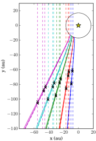
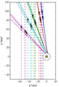
(a) Model without constraint (b) Particles going toward the observer (c) Particles going away from the observer

Figure 9: Orbiting parent body. Trajectories of the particles seen from above for the five structures in the case of a rotating parent body (see Secs. 3.2.1 and 3.2.2 for details). For each structure, five similar trajectories, sometimes superimposed, are displayed corresponding to best fits obtained when the reference structure is varied in the model. The color-coding is the same as in previous figures. The solid black circle is the trajectory of the parent body. The crosses correspond to the observing dates.

From these results, we can derive a dust release date for each of the structures for the best fit model. These are listed in Table 3.1.2 (labelled ”Orbiting free”), where the uncertainties combine the dispersion on the best ten percent pairs for a given reference structure, and the dispersion within the fits with the five different reference structures. In this model, the C structure appears first (in $\sim$1989), followed by D and E with an almost 1-year periodicity. These three trajectories point in a direction opposite to the observer. Structures A and B, on the other hand, are released much later, early 2000, about 10 to 15 years after structure E. Their trajectories are furthermore oriented toward the observer. A face-on view of the five trajectories is displayed in the left panel of Figure 9.

Although the 1-year periodicity for the C to E structures could provide some hints on the origin of the dust release process, the specific behaviour of the A and B structures is calling for staying cautious as about the interpretation of the model. This motivates us to test in the following the case of grouped release events for all the structures, in a time span shorter than a quarter of the parent body orbital period.

3.2.2 Grouped release events

We keep exploring the case of an orbiting parent body, but we now force the structures to be emitted more closely in time than previously. This is numerically achieved by limiting the accessible range of dust release dates to a quarter of the parent body orbital period. This leads to considering two situations: the case of five trajectories all oriented toward the observer on one hand, and five trajectories all moving away from the observer in the other hand.

It turns out that none of these scenarii yields better fits to the data based on a $\chi^{2}_{r}$ criterium, as one could anticipate since these situations where numerically considered in the nominal case (previous section). The best fit to the positions of the structures in time with particles forced to be emitted in the direction of the observer is shown in the middle panel of Fig. 9. It corresponds to $\beta=24.7^{+10.6}_{-2.9}$, $R_{0}=17.3^{+4.7}_{-3.0}$ au, and the corresponding dust release dates are reproduced in Table 3.1.2. The fits with different reference structures are consistent with each other. The values of $\beta$ and $R_{0}$ are significantly larger than those obtained in the nominal orbiting case (Sec. 3.2.1). The upper limit on $\beta$ is in fact reaching the upper bound of the explored range in our simulations (see Fig. 18), and we checked that expending this range increases the best $\beta$ value, as well as the corresponding $R_{0}$ value in accordance to Eq. 9. The reduced $\chi^{2}_{r}$ of about 3.6 is worse than in the nominal orbiting case, but it is interesting to note that a dust release periodicity of about 1.5 years does appear in this model, with the structures at the largest projected distances from the star being the oldest (release dates between about 1994 and 2000 for the E to A structures, respectively).

The case of particules forced to be pulled away from the observer yields quite different results. The best fit is obtained for $\beta=5.6^{+4.8}_{-3.6}$ and $R_{0}=8.1^{+2.0}_{-3.1}$ au (see Fig. 9c), with a reduced $\chi^{2}_{r}$ value around 3.5. In this case, the dispersion in the parameter values due to the use of different reference structures is larger than before, as can be seen on the right panel of Fig. 9. Overall, the mean $\beta$ and $R_{0}$ values are similar than in the nominal case (Sec. 3.2.1). The dust release dates are documented in Table 3.1.2. It shows that the periodicity is a little smaller than one year and the closest structures in projection are the oldest in this model, with structure A appearing in $\sim$1990 and the last structure (E) in $\sim$1994.

In summary, even if the grouped emission solutions are not the best based on the $\chi^{2}_{r}$ criterium, they present the conceptual advantage of a periodicity.

4 Discussion

Figure 10: Left: Likeliest values of $\beta$ depending on the model. ”2010 2014” is the nominal orbiting case (Sec. 3.2.1), ”2004 2014” is the same model taking into account the 2004 observations (Sec. 4.2.1), ”0.7 M_⊙” is the model with a stellar mass of 0.7 M_⊙ (Sec. 4.2.2), ”Front” and ”Back” are the grouped solutions (Sec. 3.2.2), ”Static” is the model of a static parent body (Sec. 3.1.1) and ”Eccentric” is the model discussed in Sec 3.1.2. Right: Same for the dust release position $R_{0}$.

4.1 Comparison between models

The simulations reproduce the general trend of increasing projected velocities of the structures with increasing distance to the star. This behaviour can be explained by an outward acceleration of the particles being pushed away by a stellar wind pressure force that significantly overcomes the gravitational force of the star. The static and nominal orbiting parent body models provide equally good fits to the data. Figure 10 provides a digest of the $\beta$ and $R_{0}$ values found in this study, along with the error bars at 1$\sigma$ and 3$\sigma$. Our model requires the stellar wind to be strong enough to achieve $\beta$ values between typically 3 and 10. In the static case, the dust seems to originate from a location just inside the planetesimal belt, at 25–30 au from the star, while in the case of an orbiting parent body, the best fit model is obtained for a dust release distance to the star $R_{0}$ of about 8 au. The release dust events are less than 30 years old, dating back to the late 1980’s for the oldest, while the most recent features would have been emitted in the mid-2000 at the latest in the case of an orbiting parent body, and as late as mid-2011 in the case of a static parent body. Some periodicity does appear in the simulations, but these depend on the model assumptions and current data are not sufficient to disentangle between the various scenarii considered in this study. For instance, the static parent body model shows a $\sim$7 year periodicity, while some 1 to 2 year periodicities are noticed when considering an orbiting parent body, with a possible 10-15 year inactivity period in the best fit model (Fig. 9a).

In the case of an unconstrained orbiting parent body, the best fit model suggests that the C structure is older than the D structure that is itself older than the E structure (Tab. 3.1.2 and Fig. 9a). The observations would naively suggest the opposite, namely that the closest structures are the youngest. Indeed, the vertical amplitude of the arch-like structures seems to decrease with increasing apparent position (Boccaletti et al. 2015), suggesting for example a damping process when the structures move outwards. The observed increase of the radial extent of the arches would also support this conclusion, although projections effects could also explain this behaviour. In fact, independent of the scenarii displayed in Fig. 9, the orientation of the trajectories with respect to the observer are such that, should the arches have the same shape, their apparent radial extent would increase with increasing projected distance to the star, as observed. This criterion does not allow to exclude one scenario, but ongoing follow up observations could constrain the orientation of the structures with respect to the line of sight.

It is also worth mentioning that the case of grouped release events toward the observer (Fig. 9b) does yield surprising results that must be taken with care. For this case, the best fits tend to be obtained for the largest possible $\beta$ values in our grid of models and extending the range of $\beta$ values does confirm this trend. However, we note that the improvement in terms of $\chi^{2}_{r}$ is limited, and that fixing for instance $\beta$ to about 6 would correspond to $R_{0}$ values close to 10 au ($\chi_{r}^{2}=4.6$, see Fig. 18a), in better agreement with the other models. Therefore, in the following discussion, we will adopt $\beta=6\pm 1$ and $R_{0}=8\pm 2$ au as representative values in the case of an orbiting parent body, independently of whether the release events are grouped or not.

Figure 11: Orbiting parent body. Left: Spatial extent of the arches if they were composed of particles with different $\beta$ values emitted at the same date. Right: Spatial extent of the structures if they were composed of particles released continuously during 0.4 year. The dashed black line corresponds to the apparent position of the parent body.

4.2 Critical assessement of the model

To assess the robustness of the model results, we evaluate in the following the impact of some assumptions on our findings.

4.2.1 Consistency with the 2004 observations

We have so far ignored the 2004 measurements since the arch-like features are not detected as such in these data sets. The presumed 2004 locations of the D and E features documented in Table 2 correspond to reported positions of brightness maxima in the literature rather than maximum elevations. On the other hand, these data greatly increase the time base and this provides an opportunity to check if the brightness maxima identified in 2004 would be consistent with the dynamics of the D and E features that we inferred. We derived best fits to the 2004, 2010, 2011 and 2014 data altogether by considering the case of an orbiting parent body, with no restriction on the period of emission, a situation similar to the nominal case in Sec. 3.2.1. The likeliest values of $\beta$ and $R_{0}$ are reported in Figure 10 for comparison with those obtained previously. We find that adding the 2004 observations reduces the error bars but has a marginal impact on the best values of the parameters (model labelled ”2004 2014” in the figures). The best fit is indeed obtained for $\beta=7.0^{+2.0}_{-1.8}$ and $R_{0}=8.2^{+0.9}_{-1.2}$ au. This compares well with the values derived from the best fit to the 2010–2014 data set, and introducing new data to the fit only yields a small increase of the reduced $\chi^{2}_{r}$ (2.4 vs 1.7). Therefore, we conclude that the 2004 brightness assymmetries in the 2004 images can be associated with structures D and E, as proposed in Boccaletti et al. (2015). A more appropriate evaluation of these features will be presented in Boccaletti et al. (in prep.).

4.2.2 Stellar parameters

A parameter that can affect the modeling results is the stellar mass. The uncertainty on the estimation of AU Mic’s mass leads us to examine the impact of an heavier star. We consider again the case of an orbiting parent body with no constraint on the emission dates as in Sec. 3.2.1, and we change the stellar mass from 0.4 M_⊙ to 0.7 M_⊙ (labelled ”0.7 M_⊙” in Fig. 10). The best value of $\beta$ is essentially not affected ($5.4^{+4.3}_{-2.5}$), but $R_{0}$ is increased to $9.7^{+1.6}_{-2.0}$ au such that the orbital period is kept nearly constant with respect to the case of a lower stellar mass. In the 0.7 M_⊙ case, the parent body has an orbital period of 36.1 years, against 33.8 years in the solution of Section 3.2.1. It means that the time interval between each dust release event is most significant than the radius of emission. Overall, it shows that the uncertainty on the mass of the star does not significantly impact our main conclusions.

Another stellar parameter that can affect the simulations is the stellar wind speed, here assumed to be equal to the escape velocity at the surface of the star, following the approach by Strubbe & Chiang (2006) and Schüppler et al. (2015). Although observations (Lüftinger et al. 2015) and models (Wood et al. 2015) exist for the stellar wind of main-sequence solar-like stars of various ages, the constraints are very scarce for an active, young M-type star like AU Mic. In the literature, the values are either computed based on the escape velocity, or by considering the temperature at the base of the open coronal field lines together with the Parker’s hydrodynamical model (1958). This leads to wind speed values that can vary by a factor of up to 3 from a model to another. We have numerically checked that multiplying by a factor of 10 our adopted value of 450 km/s for the wind speed only changes marginally the dust dynamics. This is true as long as the dust speed is neglectible with respect to the wind speed (see Sec. 2.2). As a consequence, the inferred best $\beta$ and $R_{0}$ parameters are not affected by the exact $V_{\rm sw}$ value assumed in the model. However, the connection between $\beta$ and the grain size depends on the wind speed, as discussed in Sec. 4.3.

4.2.3 $\beta$ distribution and event duration

Our model intrinsically assumes that the observed features labelled A to E are made of grains of a single size (unique $\beta$ value) and that the dust release events are sufficiently short in time to be considered as instantaneous. In the case of an orbiting parent body, the best fit value for $\beta$ shows a $1\sigma$ uncertainty of about 30%. That suggests a limited dispersion in $\beta$ values. This is illustrated in the left panel of Figure 11 where it is shown that $\Delta\beta/\beta$ of about 1/3 can be tolerated as long as the D and E features are concerned, but the model becomes increasingly inconsistent with the observations when considering the features located closer and closer to the star. For the A, B, and C structures, we observe an overlap which would connect the features, contradicting the observations. This very much suggests that either the arch-likes features are formed of grains with a narrow size distribution, and/or that their cross sectional area is dominated by grains in a narrow size range (see also Sec. 4.3).

Likewise, assuming for example that the dust release events last a few months significantly widens the range of apparent trajectories as illustrated in Figure 11 (right panel, $\Delta t=\pm 0.2$ year). However, this behaviour is still compatible with the observations, since the structures are not mixed together, and have a radial extent compatible with the one obtained here. This suggests that the emission process can occur during a few months, as long as it stay shorter than the time difference between two consecutive structures (0.6 year in this case).

Therefore, the on-going follow up on this system will be critical to further constrain the $\beta$ distribution and the duration of release events.

4.3 Grain size and mass loss rate

Figure 12: Product of the mass loss rate with the wind speed vs grain size for the likeliest values of $\beta$ obtained in our simulations. The gray areas correspond to the dispersion of $\beta$ in the orbiting cases. For simplicity, our assumed value of wind speed of 450 km/s is labelled $V_{\rm sw,\odot}$. The colored vertical lines indicate, for each observing wavelength, the range of grain sizes corresponding to the smallest grains that efficiently scatter light ($s\sim\lambda/2\pi$ ) and which should dominate the flux for any ”non-exotic” grain size distribution in the clumps (see Sec. 4.3 for details).

Our best fit value for $\beta$ (about 6.3 in the case of a free orbiting parent body) is large enough to consider that the contribution of the radiation pressure to the dynamics of the grains forming the arch-like features can be neglected. Indeed, the low luminosity of the star makes $\beta_{\rm PR}$ never exceeding 0.3 as can be seen in Fig. 10 of Augereau & Beust (2006). Therefore, we can assume $\beta\simeq\beta_{\mathrm{SW}}$, and as a consequence, the link between $\beta$ and the grain size $s$ is degenerated with the mass loss rate $\dot{M}_{\star}$ and the stellar wind speed $V_{\rm sw}$, such that $\beta\propto\dot{M}_{\star}V_{\rm sw}/s$ (Eq. 2). This is illustrated in Figure 12, using dust composition M1 of Schüppler et al. (2015) ($\rho$ = 1.78 g.cm^-3, see their Tab. 2).

In this context it is interesting to question which grain sizes are probed by the visible/NIR scattered light observations. For the purpose of the discussion, we can approximate the dimensionless scattering efficiency $Q_{\mathrm{sca}}$ by a constant for grains much larger than the observing wavelength (geometric optics, $x\gg 1$ where $x=2\pi s/\lambda$ is the size parameter), and $Q_{\mathrm{sca}}\propto x^{4}$ for small grains in the Rayleigh regime ($x\ll 1$). The differential scattering cross section, that writes $Q_{\mathrm{sca}}\pi s^{2}\mathrm{d}n(s)$, is proportional to $s^{6+\kappa}\mathrm{d}s$ for $x\ll 1$ and $s^{2+\kappa}\mathrm{d}s$ for $x\gg 1$ when considering a power law differential grain size distribution $\mathrm{d}n\propto s^{\kappa}\mathrm{d}s$ with a lower cut-off size $s_{\mathrm{min}}$. For any value of $\kappa$ such as $-7<\kappa<-3$, as for instance the classical collisional ”equilibrium” size distribution in $\kappa=-3.5$ , the scattering cross section will be dominated by grains such as $s\sim\lambda/2\pi$ (i.e. $x\sim 1$). The ranges of grain sizes that these correspond to are displayed in Figure 12 for the HST/STIS (broad-band, 0.2–1.1 $\mu$m), SPHERE/IRDIS (J-band) and SPHERE/ZIMPOL (I’-band) observations, and are typically of the order of $\sim 0.1\,\mu$m. In order for grains of this size to reach our likeliest $\beta$ value of $\sim 6$, we need the $\dot{M}_{\star}\times V_{\rm sw}$ to reach values as high as a few $10^{3}$ the solar analog. Such values are at least 20 times greater than the 50 $\dot{M}_{\odot}\times V_{\rm sw,\odot}$ derived by Schüppler et al. (2015) from collisional modelling of the overall disk. However, such very large values cannot be fully ruled out because there is a large spread of $\dot{M}_{\star}V_{\rm sw}$ estimates reported in the literature for M-type stars, including values 3 to 4 orders of magnitude larger than the solar case (see e.g. Vidotto et al. 2011, and references therein). The global trends of $\dot{M}_{\star}$ decreasing with age and increasing with stellar activity (Wood et al. 2005) favor a high mass-loss rate in the case of AU Mic.

It remains to be checked, however, whether the apparent positions and velocities are sensitive to the observing wavelength, which is difficult to conclude with current data because the spectral range of the observations is limited. With a collisional grain size distribution, one would indeed expect that the structures at visible wavelengths might be formed of smaller grains with larger $\beta$ values than the structures observed in the near-infrared (smaller $\beta$ values). An alternative would be that the size distribution is very narrow, which can be schematically described by a steep size distribution with a minimum size cutoff. For $\kappa<-7$, the scattering cross section is always dominated by the smallest grains of the size distribution ($s_{\mathrm{min}}$), regardless of the observing wavelength. In this case, the features’ measured positions and velocities would be the same at all wavelengths, and all images could be dominated by the same grain sizes, which could be much smaller than 0.1 $\mu$m and thus requiring relatively moderate $\dot{M}_{\star}V_{\rm sw}$, typically 10² the solar value. This would be consitent with the blue color of the overall disk, indicating a cross sectional area dominated by submicrometer-sized grains, while micrometer-sized grains would produce gray scattering (Augereau & Beust 2006; Fitzgerald et al. 2007; Lomax et al. subm.).

We conclude that either the features are formed of grains with a size distribution that is consistent with being collisional, thus requiring a high stellar mass-loss rate; or that they are formed of grains in a very narrow range around very small sizes ($\ll 0.1\mu$m) allowing moderate mass-loss rate but requiring a physical explanation for the presence of such a large amount of nano-grains and the relative absence of slightly bigger grains (because the size distribution is extremely peaked around $s_{\mathrm{min}}$).

4.4 Detected and undected features

4.4.1 Future positions of observed features and parent body

Our model yields constraints onto the spatial and temporal origin of the grains forming the fast-moving features. This can be used to predict the future positions of the structures and offers an opportunity to better isolate, with upcoming observations, a best scenario out of the four discussed in this study and summarized in Fig. 13. Nevertheless, this figure clearly shows that the differences in apparent positions of the features according to the various scenarii start to become significant at least a few years after the most recent data used in this paper.

The predicted positions of the features for each model are documented in Table 4. In 2020 for instance, the predicted positions differ by typically a few au (a few 0.1$\arcsec$) which is in principle large enough to reject some of the proposed scenarii. However, we warn that these plausible positions of the features are idealized and do not take into account the uncertainties on the model parameters. In summary, the apparent trajectories of the known structures need to be followed in time and can be compared to our model predictions, but this might not be enough to identify within the next few years the most realistic scenario among the four presented in this paper.

Interestingly, we note that, if its orbit is exactly seen edge-on, the unseen parent body should have transited, or will at some point transit in front of the star. In all the parent body orbiting models, we expect it to have transited during the 2000–2014 time period, if its orbit is anti-clockwise. The free orbiting case predicts that the transit occured in 2008.5, the frontward orbiting case predicts it in 2007.1 and the backward orbiting case in 2010.7. Light curves of the star taken during this period could evidence this hypothetic transit (although AU Mic is active). If the orbit is clockwise, the next transit is planned in 2026.4 in the free case, in 2062.5 in the frontward case, and in 2028.6 in the backward case.

Table 4: Prediction of position (in arcsecond) for the five structures. The uncertainties correspond to the dispersion due to the reference structure chosen.

Date	Model	A	B	C	D	E
2015.0	Static	1.04 $\pm$ 0.01	1.78 $\pm$ 0.01	3.09 $\pm$ 0.03	4.09 $\pm$ 0.04	5.55 $\pm$ 0.02
	Orbiting free	1.03 $\pm$ 0.01	1.83 $\pm$ 0.02	2.97 $\pm$ 0.04	4.08 $\pm$ 0.03	5.63 $\pm$ 0.03
	Orbiting frontward	0.98 $\pm$ 0.01	1.69 $\pm$ 0.01	3.10 $\pm$ 0.02	4.20 $\pm$ 0.02	5.62 $\pm$ 0.01
	Orbiting backward	0.99 $\pm$ 0.03	1.66 $\pm$ 0.04	3.05 $\pm$ 0.01	4.19 $\pm$ 0.02	5.65 $\pm$ 0.01
2017.0	Static	1.24 $\pm$ 0.02	2.05 $\pm$ 0.01	3.42 $\pm$ 0.05	4.44 $\pm$ 0.07	5.93 $\pm$ 0.06
	Orbiting free	1.18 $\pm$ 0.02	2.11 $\pm$ 0.03	3.23 $\pm$ 0.05	4.44 $\pm$ 0.05	6.13 $\pm$ 0.04
	Orbiting frontward	1.08 $\pm$ 0.01	1.88 $\pm$ 0.01	3.44 $\pm$ 0.02	4.63 $\pm$ 0.02	6.17 $\pm$ 0.02
	Orbiting backward	1.10 $\pm$ 0.03	1.83 $\pm$ 0.04	3.35 $\pm$ 0.01	4.60 $\pm$ 0.04	6.23 $\pm$ 0.02
2020.0	Static	1.58 $\pm$ 0.03	2.49 $\pm$ 0.01	3.93 $\pm$ 0.08	4.98 $\pm$ 0.12	6.49 $\pm$ 0.12
	Orbiting free	1.41 $\pm$ 0.04	2.55 $\pm$ 0.06	3.62 $\pm$ 0.06	4.98 $\pm$ 0.08	6.90 $\pm$ 0.06
	Orbiting frontward	1.24 $\pm$ 0.01	2.17 $\pm$ 0.02	3.95 $\pm$ 0.03	5.29 $\pm$ 0.03	6.99 $\pm$ 0.03
	Orbiting backward	1.26 $\pm$ 0.04	2.08 $\pm$ 0.04	3.80 $\pm$ 0.03	5.23 $\pm$ 0.06	7.11 $\pm$ 0.05
2025.0	Static	2.25 $\pm$ 0.04	3.28 $\pm$ 0.04	4.82 $\pm$ 0.16	5.91 $\pm$ 0.21	7.45 $\pm$ 0.53
	Orbiting free	1.81 $\pm$ 0.07	3.30 $\pm$ 0.11	4.28 $\pm$ 0.07	5.89 $\pm$ 0.12	8.18 $\pm$ 0.11
	Orbiting frontward	1.50 $\pm$ 0.01	2.66 $\pm$ 0.02	4.81 $\pm$ 0.04	6.39 $\pm$ 0.05	8.38 $\pm$ 0.04
	Orbiting backward	1.53 $\pm$ 0.04	2.50 $\pm$ 0.05	4.54 $\pm$ 0.05	6.26 $\pm$ 0.09	8.58 $\pm$ 0.10

Figure 13: Apparent positions of the features as a function of the observing date for the 4 optimal cases discussed in Sec. 3.

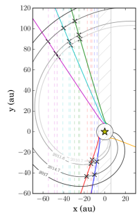
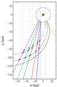
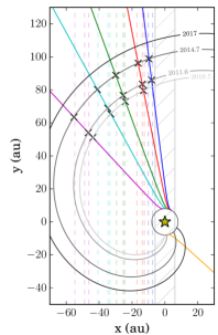
(a) Model without constraint (b) Particles going toward the observer (c) Particles going away from the observer

Figure 14: Orbiting parent body. Trajectories of the particles seen from above averaged over the five reference structures (see Secs. 3.2.1 and 3.2.2 for details). The color-coding is the same as in previous figures. The orange trajectory is the one of fictive particles released in 2012. The solid black circle is the trajectory of the parent body. The crosses correspond to the observing dates. The gray lines are the position of the dust in 2010.7, 2011.6, 2014.7 and 2017 (from the fainter to the darker), if it was continuously emitted by the parent body on its orbit. The hatched area roughly corresponds to the masked inner region in case of STIS imager.

4.4.2 Missing and future features

The observed structures are recent, and the dust release events occurred several times over the last 25–30 years. Some scenarii are characterized with a pseudo periodic behaviour, which allows us to predict new structures to appear. Therefore, it is crucial to determine whether some additional features will be, or should have been, detected. In the static case for instance, we expect any new feature to be localized on the same side of the disk (southeast), and to be emitted with an about 7-year periodicity (Sec. 3.1.1). This suggests that the next feature in the static case would be emitted in between 2018 and 2020, and the evolution of its apparent position and projected speed should be similar to feature A, but shifted in time by about 7 years. Perhaps more importantly, should any new structure be detected on the northwest side of the disk, the static parent body model would immediately be discarded.

To follow hypothetic new structures in the case of an orbiting parent body, we overplot in Figure 14 snapshots of the dust grain positions at specific observing dates as if they were emitted continuously from the parent body. In the parent body rotating frame, these positions would correspond to streaklines. At a given observing date, any previously released structure should be located on this line. In the parent body orbiting model with ungrouped released events, the model suggests a low or non-activity period between about 1990 and 2000. Structures that would have been emitted during this time period would be located between 20 and 90 au in apparent separation from the star, on the southeast side of the disk. Structures emitted after the most recent feature (feature A in about 2004) would have been too close from the star until 2012 to be detected with available instrumentation (panel (a) of Figure 14). After this date, new structures would be observable on the northwest side and would have been seen with VLT/SPHERE in 2014. Their non detection could for instance suggest that the system entered a similar inactive period as in 1990-2000.

In the scenario where all structures are moving away from the observer, the most recent structure (feature E) has been emitted late 1993, and new structures possibly emitted during the 1994–2010 time period would be observable on the southeast side of the disk, as shown on panel (c) of Fig. 14. Their non-detection suggests either the process of dust release has stopped for at least 15 years, or the dust release process is much less efficient during that time interval, making the structures not observable (too faint, for example). Following the 2014 streakline, we also notice that no structure could be located further than 70 au from the star in apparent separation in the images used in this study. The features possibly emitted after about 2010 would have been too close to the star to be detected until now, and this model predicts that new features could become observable on the northwest side of the disk in upcoming observations.

In the case of an orbiting parent body with grouped emissions toward the observer, the oldest structure was emitted in late 1993. Older features would be located beyond the E structure in projection, and could have been too faint to be detected. Therefore, this model is consistent with the lack of more distant features in the HST/STIS images (the VLT/SPHERE field of view is limited to 6”), despite a possible 1.5 to 2 year pseudo-periodicity (Sec. 3.2.2). The model also suggests that the most recent structure (feature A) is emitted in 2000, and panel (b) of Figure 14 shows that any feature formed during the 2000–2010 time period would be essentially lying along the line of sight to the star, yielding very small projected separations, preventing their detection with the VLT/SPHERE and HST/STIS images used in this paper. Therefore, the parent body could have continued emitting periodically since 2000 while remaining consistent with the non-detection of additional features. We note however that GPI observations by Wang et al. (2015) identified a source possibly corresponding to a compact clump of dust, within the apparent position of the A feature, and that would be consistent with a new structure emitted in 2001.1. Structures possibly emitted after 2011 should have been observed on the northwest side of the disk in 2014 (see for example the orange trajectory for the position of hypothetic structures arbitrarily emitted in 2012). This suggests again that either the pseudo-periodicity is too loose to predict precisely the arrival of future structures, or that the emission process has stopped. We note, however, that this orbiting parent body model remains the most consistent with a periodic behaviour and the lack of detected features on the northwest side of the disk so far. Here again, a systematic monitoring is the key to address the actual evolution of the system.

5 Conclusion

We construct a model to reproduce the apparent positions of the structures observed in the debris disk of AU Mic, taking into account the stellar wind and radiative pressure onto the dust grains, assuming that we observe the proper motion of the dust. We do not investigate the possible physical process at the origin of the dust production, but consider two different dynamical configurations for the release of the observed dust: a common origin from a fixed location static with respect to the observer, or release from an hypothetical parent body on a Keplerian orbit. In all cases, we find that the dust seems to originate from inside the planetesimal belt, at typically 8 au from the star in the best orbiting-parent-body model, or 28 au in the static case. The high projected velocities mesured for each structure require that the observed grains have a high value of $\beta$ ($\sim 6$), the ratio of pressure and radiative forces on the gravitational force. Our study could not disentangle between all the scenarii considered based on the available observations. However, we are able to predict, for each scenario, the future behaviour of the structures and we discuss the hypothetic appearence of new structures, especially on the northwest side of the disk. For all the scenarii, we find a semi-periodic behaviour of dust release. We could also associate the brightness maxima observed in the 2004 images with the fast-moving structures resolved in the more recent high-contrast images. We suggest that the arch-like structures are either formed from $\sim 0.1\leavevmode\nobreak\ \mu$m-sized grains if the stellar wind is very strong, or from nanometer-sized grains ($\lesssim 20$ nm) with a very narrow size distribution, in the case of a more moderate stellar activity.

Our model does not provide direct constraints on the source of dust (parent body) nor on the circumstances that yield to a release event. We can however say that it must be somewhat periodic, and that every release event should last less than 6 months. Furthermore, it must produce a great amount of submicron-sized grains, possibly with a narrow size distribution. Our static parent body model could correspond to planetesimals and dust formed after a giant collision, while an orbiting parent body could correspond to an unseen planet or a local concentration of dust due to resonant trapping with a planet, for instance. A process of accretion onto the parent body, leading to ejection (see e.g. Joergens et al. 2013) can also be the origin of dust. The stellar wind plays a key role in our model and it is likely that the dust release events from the parent body are linked to the stellar activity. The stellar flares themself are much too frequent to be the triggering process responsible for the feature formation. We speculate that this could be linked to the inversion of the magnetic field sign of AU Mic, and could help forming arches (Sezestre & Augereau 2016; Chiang & Fung 2017). Overall, this model gives the base to a more complex model taking into account the vertical elevation of the structures that we will address in a future paper.

Appendix A Figures

Figure 15: Static parent body. Trajectories of the particles seen from above that best fit the apparent positions (dashed lines, color-coding similar to Fig. 6b,d) of five structures A, B, C, D and E in the case of a static parent body. It corresponds to the trajectories plotted in black in Fig. 6d, namely ($R_{0}$, $\beta$, $\theta$) = (28 au, 10.4, 165$\degr$) and (12 au, 10.4, 43$\degr$). The line of sight of observer is assumed to lie along the $y$-axis, in the direction of increasing $y$ values, with the northeast side of the disk being on the left.

Figure 16: Orbiting parent body. Normalized probability distributions of $\beta$. The vertical black line is the mean value, and the dashed area corresponds to the 1$\sigma$ distribution.

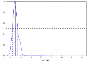
Figure 17: Orbiting parent body. Normalized probability distributions of $R_{0}$.

Table 5: Positions and speeds of the five structures (A to E) at different epochs derived from the data documented in Tab. 2. Any position corresponds to a mean value over time. The values in this table are plotted in Figure 2.

Epoch	Variable	A	B	C	D	E
2004-2010	x (au)	-	-	-	29.01	39.15
	$\delta$x (au)	-	-	-	0.58	0.90
	V (km/s)	-	-	-	6.91	11.02
	$\delta$V (km/s)	-	-	-	0.98	1.52
2004-2011	x (au)	-	-	-	29.62	40.42
	$\delta$x (au)	-	-	-	0.55	0.77
	V (km/s)	-	-	-	6.81	11.26
	$\delta$V (km/s)	-	-	-	0.81	1.17
2004-2014	x (au)	-	-	-	32.62	43.38
	$\delta$x (au)	-	-	-	0.57	0.36
	V (km/s)	-	-	-	7.56	10.62
	$\delta$V (km/s)	-	-	-	0.59	0.50
2010-2011	x (au)	-	13.14	24.91	34.09	47.56
	$\delta$x (au)	-	0.16	0.19	0.23	1.13
	V (km/s)	-	6.29	4.78	6.14	12.79
	$\delta$V (km/s)	-	1.59	1.96	2.35	11.44
2010-2014	x (au)	-	14.78	26.94	37.10	50.53
	$\delta$x (au)	-	0.18	0.31	0.27	0.90
	V (km/s)	-	5.36	5.91	8.56	10.01
	$\delta$V (km/s)	-	0.44	0.73	0.65	2.13
2011-2014	x (au)	8.78	15.40	27.41	37.71	51.79
	$\delta$x (au)	0.12	0.16	0.27	0.19	0.78
	V (km/s)	4.10	5.07	6.25	9.30	9.16
	$\delta$V (km/s)	0.38	0.49	0.84	0.60	2.40

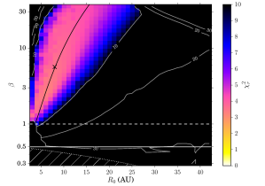
(a) Forward case (b) Backward case

Figure 18: Orbiting parent body. $\chi^{2}_{r}$ maps for the grouped release cases.