Stochastic locality and master-field simulations of very large
lattices

Abstract

In lattice QCD and other field theories with a mass gap, the field variables in distant regions of a physically large lattice are only weakly correlated. Accurate stochastic estimates of the expectation values of local observables may therefore be obtained from a single representative field. Such master-field simulations potentially allow very large lattices to be simulated, but require various conceptual and technical issues to be addressed. In this talk, an introduction to the subject is provided and some encouraging results of master-field simulations of the SU(3) gauge theory are reported.

1 Introduction

Numerical simulations of Euclidean lattice field theories usually proceed by generating an ensemble of representative fields through a Markov process. The ensemble averages of the observables of interest then provide stochastic estimates of their field-theoretical expectation values.

In lattice QCD, the field variables in distant regions of a physically large lattice fluctuate largely independently, a property that may be referred to as “stochastic locality”. Moreover, assuming periodic boundary conditions, their distribution is everywhere the same. The translation averages

$$\langle\!\langle{\mathcal{O}}(x)\rangle\!\rangle=\frac{1}{V}\sum_{z}{\mathcal{O}}(x+z)$$ (1)

of local observables ${\mathcal{O}}(x)$ (where $V$ denotes the number of lattice points and $z$ runs over the lattice) are thus expected to coincide with their field-theoretical expectation values,

$$\langle\!\langle{\mathcal{O}}(x)\rangle\!\rangle=\langle{\mathcal{O}}(x)\rangle+{\rm O}(V^{-1/2}),$$ (2)

up to statistical errors of order $V^{-1/2}$. These formulae also apply in the case of Wilson loops, products of local fields and other non-local observables, provided their localization range is much smaller than the linear extent of the lattice. On very large lattices, accurate results for the expectation values of all these observables may therefore conceivably be obtained from a single representative field.

Such master-field simulations need not require astronomical computer resources. The computer time required for the generation of $256$ statistically independent field configurations on an $L^{4}$ lattice or of a single field on a $(4L)^{4}$ lattice is roughly the same. Master-field simulations of QCD on lattices with $256^{4}$ points and physical extent in the range from $12$ to $25$ fm, for example, may thus very well be practically feasible at present and would obviously be very interesting. In this talk, various technical aspects of this new type of simulations are addressed and some first numerical studies are presented for illustration.

2 Statistical error estimation

The statistical errors of ensemble averages of the observables of interest are usually estimated from the variances and statistical correlations of the measured values of the observables UlliError . In master-field simulations, where the generated ensemble of fields contains a single field or at most a few fields on a physically large lattice, the error estimation must proceed in a different way. In particular, the correlations of the field variables in space must be taken into account.

2.1 Single-field error formula

Let ${\mathcal{O}}(x)$ be an observable localized in a region centered at the point $x$. For the derivation of the error formula it is helpful to imagine that a long simulation has been performed. The translation averages $\langle\!\langle{\mathcal{O}}(x)\rangle\!\rangle$ of the observable calculated in the course of the simulation are then distributed according to their field-theoretical distribution. In the limit of an infinitely long run, their average thus coincides with $\langle{\mathcal{O}}(x)\rangle$ and their mean square deviation from the average is given by

$$\bigl{\langle}\{\langle\!\langle{\mathcal{O}}(x)\rangle\!\rangle-\langle{\mathcal{O}}(x)\rangle\}^{2}\bigr{\rangle}=\frac{1}{V}\sum_{y}\langle{\mathcal{O}}(y){\mathcal{O}}(0)\rangle_{\rm c}.$$ (3)

In this equation, use has been made of the periodic boundary conditions and the translation invariance of the two-point correlation function of the observable. The subscript “c” indicates that the correlation function is the connected one.

Equation (3) provides an exact expression for the average mean square deviation of the translation average $\langle\!\langle{\mathcal{O}}(x)\rangle\!\rangle$ from the field-theoretic expectation value $\langle{\mathcal{O}}(x)\rangle$ in a master-field simulation. Since the correlation function in this expression falls off exponentially at large distances, the formula shows that the statistical errors in these simulations do in fact decrease proportionally to $V^{-1/2}$ as $V\to\infty$. Moreover, the proportionality constant is seen to be determined by the two-point correlation function of the observable considered and thus depends on the localization range of the latter and the relevant correlation lengths.

As it stands, Eq. (3) is not particularly useful, since the correlation function on the right is usually not known. One may, however, sum the correlation function up to some radius $R$,

$$\bigl{\langle}\{\langle\!\langle{\mathcal{O}}(x)\rangle\!\rangle-\langle{\mathcal{O}}(x)\rangle\}^{2}\bigr{\rangle}=\frac{1}{V}\Bigl{\{}\sum_{|y|\leq R}\langle{\mathcal{O}}(y){\mathcal{O}}(0)\rangle_{\rm c}+{\rm O}({\rm e}^{-mR})\Bigr{\}},$$ (4)

at the expense of an exponentially small systematic error, $m$ being some mass that characterizes the decay of the correlation function at large distances. The replacement of the correlation function through the corresponding translation average then leads to a formula

$$\bigl{\langle}\{\langle\!\langle{\mathcal{O}}(x)\rangle\!\rangle-\langle{\mathcal{O}}(x)\rangle\}^{2}\bigr{\rangle}=\frac{1}{V}\Bigl{\{}\sum_{|y|\leq R}\langle\!\langle{\mathcal{O}}(y){\mathcal{O}}(0)\rangle\!\rangle_{\rm c}+{\rm O}({\rm e}^{-mR})+{\rm O}(V^{-1/2})\Bigr{\}}$$ (5)

suitable for numerical evaluation. The last term on the right of this equation, i.e. the statistical “error of the error”, could be expressed through the four-point function of ${\mathcal{O}}(x)$ in a way similar to the error itself. Clearly, Eq. (5) assumes the existence of a window of values of $R$, where both the systematic error and the statistical error of the error are negligible.

2.2 Several master fields

In the case of a (usually small) ensemble $\{U_{1},\ldots,U_{n}\}$ of master fields, generated by letting the simulation algorithm run for some length of time, one first calculates the ensemble average

$$\overline{\vphantom{(}{\mathcal{O}}}(x)=\frac{1}{n}\sum_{k=1}^{n}\left.{\mathcal{O}}(x)\right|_{U=U_{k}}$$ (6)

of the observable ${\mathcal{O}}(x)$. The translation average $\langle\!\langle\overline{\vphantom{(}{\mathcal{O}}}(x)\rangle\!\rangle$ then provides an estimate of the expectation value $\langle{\mathcal{O}}(x)\rangle$ with variance

$$\bigl{\langle}\{\langle\!\langle\overline{\vphantom{(}{\mathcal{O}}}(x)\rangle\!\rangle-\langle{\mathcal{O}}(x)\rangle\}^{2}\bigr{\rangle}=\frac{1}{V}\Bigl{\{}\sum_{|y|\leq R}\langle\!\langle\overline{\vphantom{(}{\mathcal{O}}}(y)\overline{\vphantom{(}{\mathcal{O}}}(0)\rangle\!\rangle_{\rm c}+\ldots\,\Bigr{\}},$$ (7)

provided the autocorrelation functions of the observable are translation invariant and decay rapidly at large distances in space. These technical requirements are usually satisfied and certainly so, if the simulation algorithm is in the universality class of the (position-space) Langevin equation.

Clearly, if the fields $U_{1},\ldots,U_{n}$ are statistically independent, the variance (7) is exactly $n$ times smaller than the variance in the case of a single master field. Equation (7) however remains valid in presence of statistical correlations and these need not be determined, i.e. they are automatically taken into account and only the terms represented by the ellipsis depend on them.

2.3 Selected remarks

2.3.1 Application of the fast Fourier transform (FFT)

The correlation function on the right of the error formula (5),

$$\sum_{|y|\leq R}\langle\!\langle{\mathcal{O}}(y){\mathcal{O}}(0)\rangle\!\rangle_{\rm c}=\frac{1}{V}\sum_{|y|\leq R}\sum_{z}\bigl{(}{\mathcal{O}}(y+z)-\langle\!\langle{\mathcal{O}}(y)\rangle\!\rangle\bigr{)}\bigl{(}{\mathcal{O}}(z)-\langle\!\langle{\mathcal{O}}(0)\rangle\!\rangle\bigr{)},$$ (8)

may be evaluated in two steps. Assuming ${\mathcal{O}}(z)$ is known at all lattice points, the sum over $z$ can first be performed for all $y$ simultaneously using the FFT. The sum over $y$ may then be evaluated for all $R$ in the chosen range of values. As $V\to\infty$, the numerical effort required for the calculation of the sums in Eq. (8) thus scales like $V\ln V$.

2.3.2 “Dilute data”

In practice an observable ${\mathcal{O}}(z)$ may only be known on a sublattice of points $z$. The translation averages are, in these cases, taken over the sublattice and the sums in the error formulae then run over the sublattice too. Depending on the correlations of the observable in space, the restriction to the sublattice may or may not have a significant influence on the statistical errors.

2.3.3 Error correlations and propagation

The error formulae derived in this section straightforwardly generalize to the case of the statistical correlations of two or more primary observables. Bootstrap methods then provide a computationally efficient and convenient way to propagate the statistical errors to any secondary observables.

3 Sample calculations

The master-field simulations of the SU(3) gauge theory reported in this section mainly serve to demonstrate that the error formulae derived in the previous section work out in practice. In all cases, the Wilson plaquette action Wilson was used and the gauge fields were generated with the SMD algorithm (see sect. 4). Lattices of size up to $192^{4}$, with spacing $a$ equal to $0.10$ or $0.05$ fm, were simulated. The simulations of the largest lattices occupied $64$ nodes ($1536$ cores, $8.2$ TB total memory) of the FinisTerrae II machine at CESGA for about 10 days.

3.1 Reference flow time

Among the most easily accessible renormalized quantities in the pure gauge theory are the Yang-Mills action density $E(x)$ at gradient-flow time $t>0$ and the reference scale $t_{0}$ that derives from the latter WilsonFlow ; RenFlow . The action density $E(x)$ is a primary observable localized in a ball centered at $x$ with radius roughly equal to $\sqrt{8t}$ (at flow times near $t_{0}$, this is about $0.5$ fm in physical units).

Figure 1: Relative statistical error $\sigma$ of $\langle\!\langle E(x)\rangle\!\rangle$ at gradient-flow time $t\simeq t_{0}$, as determined by the first term on the right of the error formulae (5) and (7), respectively. The lines connecting the data points are drawn to guide the eyes. Except for the data labeled “avg”, which are obtained from an ensemble of $13$ fields, the data are from different single fields (the numbering of the fields corresponds to the one in Fig. 2).

The calculations of the action density and of the reference flow time reported here were performed on lattices of size $96^{4}$ and $192^{4}$ with spacing $a=0.10$ fm. On these lattices and at $t\simeq t_{0}$, the statistical errors of $\langle\!\langle E(x)\rangle\!\rangle$ safely reach a plateau as a function of the summation radius $R$ used in the error formulae (see Fig. 1). There is a small difference in the plateau height obtained in the case of the fields no 1 and 2, which gives an indication of the size of the error of the error on the $96^{4}$ lattice. Averaging the values of $E(x)$ measured on $n=13$ weakly correlated configurations has the expected effect of lowering the statistical error by the factor $n^{-1/2}$ (points labeled “avg” in Fig. 1). Even smaller errors are obtained when the lattice size is increased from $96^{4}$ to $192^{4}$. The (relative) error of the error then also goes down by about a factor $4$.

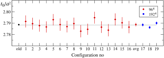
Figure 2: Values of the reference flow time $t_{0}$ obtained in master-field simulations. The point labeled “old” is from a previous traditional simulation CeEtAlTop and the one labeled “avg” from an ensemble of $13$ fields on the $96^{4}$ lattice. A least-squares fit of the single-field results was used to produce the horizontal line.

As shown by Fig. 2, the results for the reference flow time $t_{0}$ obtained in the master-field simulations reported here are statistically compatible among themselves and with an earlier traditional calculation. Given the estimated statistical uncertainties, the scattering of the points is certainly plausible and thus supports the conclusion that the errors are correctly estimated.

3.2 Topological susceptibility

Following ref. WilsonFlow , the topological susceptibility is defined by

$$\chi_{t}=\sum_{y}\langle q(y)q(0)\rangle,$$ (9)

where $q(x)$ is a lattice expression for the topological charge density at gradient-flow time $t>0$. In the tests conducted here, the so-called symmetric (“clover”) expression was used for the charge density and $t$ was set to the reference flow time $t_{0}$.

On large lattices, the susceptibility may be calculated by splitting the sum over $y$ in two parts,

$$\chi_{t}=\sum_{|y|\leq R}\langle q(y)q(0)\rangle+\delta(R)=\sum_{|y|\leq R}\langle\!\langle q(y)q(0)\rangle\!\rangle+\delta(R)+{\rm O}(V^{-1/2}),$$ (10)

where

$$\delta(R)=\sum_{|y|>R}\langle q(y)q(0)\rangle$$ (11)

is rapidly decaying at large $R$. The replacement of the field-theoretical correlation function in Eq. (10) by the translation average of the observable

$${\mathcal{O}}(x)=\sum_{|y|\leq R}q(x+y)q(x)$$ (12)

adds a statistical error of order $V^{-1/2}$ to the expression. A calculation of the susceptibility along these lines assumes that there exist values of $R$, where the systematic error $\delta(R)$ is small and which are much smaller than the linear extent of the lattice so that the statistical error is small too.

Master-field simulations are, by definition, simulations where the topological charge of the gauge field assumes some fixed value. Fixed-topology simulations are known to give results for local correlation functions that differ from their exact field-theoretical values by terms of order $V^{-1}$ BrowerEtAl ; AokiEtAl . These effects are parametrically smaller than the statistical errors, which shows that master-field simulations provide a solution to the infamous topology-freezing problem in lattice QCD if the physical size of the lattice is large enough.

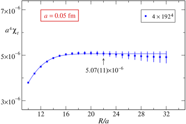
Figure 3: Master-field estimates of the topological susceptibility through the translation average of the observable (12) at two values of the lattice spacing. The smooth curves represent a fit of the data by a constant plus a deviation of the form (13). In these calculations, the systematic errors (11) are estimated to be negligible with respect to the statistical errors at $R/a\geq 13$ and $R/a\geq 22$, respectively.

As a function of the summation radius $R$, the first term on the far right of Eq. (10) reaches a plateau at about $0.8$ fm (see Fig. 3). Reflection positivity implies that the second term $\delta(R)$ is negative at asymptotically large values of $R$, but its analytic form is not known and certainly strongly influenced by the gradient-flow smoothing in the range of $R$, where the data in Fig. 3 significantly depart from the plateau value. The deviation is actually well represented by

$$\delta(R)=b\int_{|y|\geq R}{\rm d}^{4}y\,{\rm e}^{-cy^{2}}$$ (13)

in that range, with fitted parameters $b$ and $c$.

The results for the topological susceptibility in lattice units quoted in Fig. 3 coincide, within errors, with the values $7.884(9)\times 10^{-5}$ CeEtAlTop and $4.98(30)\times 10^{-6}$ ChowdhuryEtAl previously obtained at $a=0.10$ and $0.05$ fm, respectively, using traditional methods. At $a=0.10$ fm the results are very precise and their agreement is thus particularly impressive. It might however be difficult to reach a similar precision at $a=0.05$ fm with traditional simulations in view of the long autocorrelation times of the topological charge. Master-field simulations effectively bypass the problem and yield results with constant relative precision as $a\to 0$, if the lattice volume is held fixed in physical units.

3.3 Correlation function of the action density

The calculation of the connected correlation function of the Yang–Mills action density $E(x)$ in master-field simulations is, in principle, straightforward. As is the case in ordinary simulations, the signal-to-noise ratio decreases exponentially at large distances and projections to a definite spatial momentum further increase the statistical noise proportionally to the square root of the three-dimensional volume (see ref. KehFei for a recent discussion of the problem). The increase of the statistical noise through the momentum projection is however less severe in the case of hadron propagators without disconnected parts. Here the issue is avoided by considering the point-to-point correlation function of the action density.

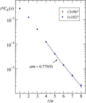
Figure 4: Master-field simulation results for the correlation function (15) of the action density at $a=0.10$ fm and gradient-flow time $t=0.36\times t_{0}$. The points obtained on the $96^{4}$ and $192^{4}$ lattices lie practically on top of each other. The full line represents an uncorrelated least-squares fit of the data on the larger lattice to the expected asymptotic form (20) of the correlation function. In the fit range, the statistical errors of $t^{4}C_{E}(r)$ determined by Eq. (18) are roughly constant and equal to $3.1\times 10^{-7}$ at $r/a=8$.

Since the latter includes a non-zero disconnected contribution, the calculation requires two primary observables, ${\mathcal{O}}_{1}(x)$ and ${\mathcal{O}}_{2}(x)$, to be chosen, one for the connected and the other for the disconnected part. In the present context, the observables should have a minimal localization range centered at $x$. Moreover, assuming an $L^{4}$ lattice, one would like to take advantage of the hyper-cubic symmetry of the lattice theory to reduce the statistical errors.

Considering these requirements, a possible choice of observables is

$${\mathcal{O}}_{1}(x)=\hbox{\normalsize$\frac{1}{4}$}\sum_{\mu=0}^{3}E(x+h_{+}\hat{\mu})E(x-h_{-}\hat{\mu}),\quad{\mathcal{O}}_{2}(x)=\hbox{\normalsize$\frac{1}{8}$}\sum_{\mu=0}^{3}\bigl{\{}E(x+h_{+}\hat{\mu})+E(x-h_{-}\hat{\mu})\bigr{\}},$$ (14)

where $\hat{\mu}$ denotes the unit vector in direction $\mu$ and the displacements $h_{\pm}$ are integer multiples of the lattice spacing. The (on-axis) correlation function at distance $r=h_{+}+h_{-}$ is then given by

$$C_{E}(r)=\langle\!\langle{\mathcal{O}}_{1}(x)\rangle\!\rangle-\langle\!\langle{\mathcal{O}}_{2}(x)\rangle\!\rangle^{2}$$ (15)

up to statistical errors of order $V^{-1/2}$. In order to minimize the localization region of the observables, $h_{+}$ is set to $r/2$ if $r$ is an even multiple of the lattice spacing and to $(r+a)/2$ otherwise.

The square of the associated statistical error,

$$\sigma_{E}(r)^{2}=\sum_{k,l=1}^{2}w_{k}w_{l}\,\hbox{cov}_{kl}(r),\quad w_{1}=1,\quad w_{2}=-2\langle\!\langle{\mathcal{O}}_{2}(x)\rangle\!\rangle,$$ (16)

is determined by the standard error-propagation rules and the $2\times 2$ covariance matrix

$$\hbox{cov}_{kl}(r)=\frac{1}{V}\sum_{|y|\leq R}\langle\!\langle\hat{{\mathcal{O}}}_{k}(y)\hat{{\mathcal{O}}}_{l}(0)\rangle\!\rangle,\quad\hat{{\mathcal{O}}}(x)\equiv{\mathcal{O}}(x)-\langle\!\langle{\mathcal{O}}(x)\rangle\!\rangle,$$ (17)

(with a properly chosen value of the summation radius $R$) of the primary observables. Insertion of Eq. (17) in Eq. (16) followed by a few lines of algebra then lead to the error formula

$$\sigma_{E}(r)^{2}=\frac{1}{V}\sum_{|y|\leq R}\langle\!\langle\tilde{{\mathcal{O}}}_{1}(y)\tilde{{\mathcal{O}}}_{1}(0)\rangle\!\rangle_{\rm c},\quad\tilde{{\mathcal{O}}}_{1}(x)\equiv\hbox{\normalsize$\frac{1}{4}$}\sum_{\mu=0}^{3}\hat{E}(x+h_{+}\hat{\mu})\hat{E}(x-h_{-}\hat{\mu}),$$ (18)

which is easy to memorize given that Eq. (15) may be written in the form

$$C_{E}(r)=\langle\!\langle\tilde{{\mathcal{O}}}_{1}(x)\rangle\!\rangle.$$ (19)

In the case of several master fields, the same formulae hold with ${\mathcal{O}}_{1}(x)$ and ${\mathcal{O}}_{2}(x)$ replaced by their ensemble averages (cf. subsect. 2.2).

At large distances, the correlation function decays exponentially,

$$C_{E}(r)\mathrel{\mathop{\propto}_{r\to\infty}}r^{-3/2}{\rm e}^{-mr},$$ (20)

where $m$ is the mass of the lightest scalar glueball. The data shown in Fig. 4 can actually be accurately represented by this asymptotic expression at distances $r\geq 0.4$ fm. Clearly, more reliable determinations of the scalar glueball mass would require the master-field simulations to be combined with other techniques such as the variational method and multilevel measurement algorithms.

4 Generation of master fields

The derivation of the error formulae in sect. 2 shows that any correct simulation algorithm may in principle be used for the generation of master fields. If only a single field is generated, all the computational work is done in what is often referred to as the “thermalization phase” in ordinary simulations. Several fields are generated as usual by running the algorithm for some length of time after thermalization. There are, however, important technical issues that must be addressed, some concerning the thermalization phase and others the use of global operations, which tends to be problematic on very large lattices.

4.1 Thermalization

4.1.1 Building configurations from small lattices

In order to reduce the computer time spent in the thermalization phase, it is common practice to construct the initial fields from thermalized fields on smaller lattices through periodic extension. Lattice extensions may proceed in several steps, from one lattice size to the next with intermediate thermalization runs, if initial fields for simulations of very large lattices are constructed.

The topological charge of the fields generated in this way however tends to grow proportionally to the lattice volume $V$, particularly so when the autocorrelation time of the charge is larger than the length of the intermediate thermalization runs. For fixed-topology effects to be of order $V^{-1}$, the value of the charge must be in the central range of the exact charge distribution BrowerEtAl ; AokiEtAl . Since the width of the distribution is of order $V^{1/2}$, this condition is then likely to be violated.

The problem can easily be avoided by extending the fields through reflections at the lattice planes rather than periodically. In this case, a duplication of the field in one or more dimensions, for example, produces a field with vanishing topological charge. One then ends up with master fields that satisfy the condition mentioned above with high probability.

4.1.2 Autocorrelations

To be able to judge whether the simulation has reached its asymptotic stationary state, the autocorrelation times of a representative set of observables must be known. Very accurate calculations of the autocorrelation times are not required and the possibly very large autocorrelation times of the topological charge can be ignored, since master-field simulations are anyway fixed-topology simulations. A sensible measure of autocorrelations, which may be used in this context, are the distances in simulation time, where the autocorrelation functions of the observables considered have decreased by, say, a factor $2$. These are easier to determine than the integrated autocorrelation times and less sensitive to any long tails of the autocorrelation functions caused by the freezing of the topological charge.

If a simulation algorithm is used that updates the field variables in physically distant regions essentially independently, as does the SMD algorithm discussed below, the autocorrelation functions of local observables can be expected to decay rapidly in space. Under these conditions, it is plausible that the autocorrelation times of observables with localization ranges up to a few times the basic correlation lengths capture the dynamics of the algorithm sufficiently well. Moreover, in the large-volume regime of QCD, their autocorrelation times should be weakly dependent on the lattice size (if the parameters of the theory and the algorithm are held fixed). They can, therefore, be estimated on lattices much smaller than the ones considered for the master-field simulations, where long simulations may be unaffordable.

4.2 Global operations

The use of global branch conditions and other global constructions is unnatural in local theories and should be reconsidered when very large lattices are simulated. Their implementation may, in any case, be increasingly challenging in large volumes for purely technical reasons.

4.2.1 Solver stopping criterion

At present all widely used algorithms for the solution of the lattice Dirac equation are Krylov space solvers with various preconditioners. If $D$, $\eta$ and $\psi$ denote the lattice Dirac operator, source field and current approximate solution of the equation, the solver program exits when the bound

$$\|\eta-D\psi\|_{2}\leq\rho\,\|\eta\|_{2},\qquad\|\eta\|^{2}_{2}\equiv\sum_{x}\eta(x)^{\dagger}\eta(x),$$ (21)

is satisfied, where the tolerance $\rho$ is some fixed small number such as $10^{-12}$.

The stopping criterion (21) alone does not guarantee that the residues $(\eta-D\psi)(x)$ of the calculated solutions are uniformly small. In lattice QCD simulations, where the norm of the source fields grows like $V^{1/2}$ with the lattice volume, large local inaccuracies of the solutions (and thus of the quark forces) are not excluded and might compromise the simulations. In principle the growth of the norm of the sources with the lattice size could be compensated by reducing the tolerance $\rho$, but the loss of significance in the calculation of the residues sets a lower limit (of about $10^{-14}$ if the fields are stored with 64 bit precision) on the tolerances that can be imposed in practice.

On very large lattices, the norm in Eq. (21) should thus be replaced by a uniform norm such as

$$\|\eta\|^{2}_{\infty}=\max_{x}\bigl{\{}\eta(x)^{\dagger}\eta(x)\bigr{\}}$$ (22)

and solvers for the Dirac equation must then be developed, which converge to uniformly accurate solutions. Alternating Schwarz procedures, local deflation and other algorithms that proceed locally are likely elements of such solvers, but much work will no doubt be required to find the right combinations of these methods.

4.2.2 HMC accept-reject step

Global decisions are also taken in the accept-reject step of the HMC algorithm, which corrects for the inexact numerical integration of the molecular-dynamics equations HMC . More precisely, the fields obtained at the end of the molecular-dynamics evolution are accepted with probability

$$P_{\rm acc}=\min\{1,{\rm e}^{-\Delta H}\},$$ (23)

where $\Delta H$ is the difference of the values of the Hamilton function at the beginning and the end of the evolution. If an integration scheme of order $p$ is used, $\Delta H$ roughly scales like

$$\Delta H\propto\epsilon^{p}V^{1/2}$$ (24)

with the integration step size $\epsilon$ and the lattice volume $V$. In order to preserve a reasonable acceptance rate, the step size must therefore be reduced proportionally to $V^{-1/2p}$ if the lattice volume is increased. More worrisome is the fact that there is a loss of significance proportional to $V$ when $\Delta H$ is calculated. On large lattices, the point where $\Delta H$ is obtained with barely any significant digits may then rapidly be reached if the fields are stored with 64 bit precision.

Both problems can be avoided by localizing the algorithm, i.e. by updating the field variables in subvolumes rather than all field variables at once. In the case of the pure gauge theory, for example, the link variables in any rectangular block of lattice points can be updated with the HMC algorithm, while keeping the other field variables fixed. The localization of the simulation is however highly non-trivial in presence of the sea quarks and it is only recently that a viable solution to the problem was found by Cè, Giusti and Schaefer Multilevel . So far the localized algorithm has been described for divisions of the lattice in (thick) time slices, but it is quite clear that algorithms localized in four dimensions can be constructed along the same lines.

4.3 SMD algorithm w/o accept-reject step

Simply dropping the accept-reject step is another possibility worth considering. The algorithm then becomes inexact and its long-time behaviour thus needs to be understood as well as the effects of the integration errors on the calculated expectation values. In the following, the stochastic-molecular-dynamics (SMD) algorithm Horowitz ; JansenLiu is discussed, which is closely related to the HMC algorithm and similarly efficient OpenBC , but more easily accessible to rigorous mathematical analysis.

4.3.1 SMD algorithm

The SMD algorithm largely coincides with the HMC algorithm. An update cycle starts with a refreshment of the momentum field $\pi$ and the pseudo-fermion fields $\phi$ (if any) according to

$$\pi \to c_{1}\pi+c_{2}\upsilon,\qquad c_{1}={\rm e}^{-\gamma\epsilon},\quad c_{1}^{2}+c_{2}^{2}=1,$$

$$\phi \to c_{1}\phi+c_{2}\chi,$$ (25)

where $\upsilon$ and $\chi$ are random momentum and pseudo-fermion fields with the appropriate Gaussian distributions. The algorithm has two parameters, the friction constant $\gamma$ and the simulation step size $\epsilon$, which are both assumed to be positive. In the second step of the update cycle, the molecular-dynamics equations for the momentum and the gauge field are integrated from the current simulation time $t$ to $t+\epsilon$. The accept-reject step normally applied at the end of the molecular-dynamics evolution is omitted here and the algorithm instead proceeds with the next update cycle.

The simulation step size $\epsilon$ is usually set to a fraction of unity and $\gamma$ is taken to be such that the accumulated refreshment of the fields practically amounts to a complete refreshment after running the algorithm for a few units of simulation time. Any symplectic reversible integrator, such as the highly efficient ones described in ref. OMF , may be used for the numerical integration of the molecular-dynamics equations.

4.3.2 Existence and uniqueness of a stationary state

Stochastic processes like the SMD algorithm need not converge to a unique stationary state. They can run away in non-compact directions of the field space, for example, or their long-time behaviour may depend on the initial distribution of the fields. Moreover, in the case of the SMD algorithm, there is no explicitly known candidate for the equilibrium distribution if the accept-reject step is dropped.

The theory of Markov processes on field spaces (and more general spaces) is a well developed and active research area in mathematics. In particular, there exists a form of Harris’ convergence theorem, established by Hairer and Mattingly HairerMattingly , which may be applied in the present context. Some work is however still required to show that the premises of the theorem are fulfilled SMDergodicity .

As a result one obtains a rigorous proof of the convergence of the SMD algorithm to a unique stationary state at large simulation times, assuming the following properties hold:

• The gauge action is a smooth function of the link variables.

• Sea quarks (if any) are included in the standard way, with operators in the pseudo-fermion actions that are bounded, strictly positive and smoothly dependent on the gauge field .

• A symplectic integrator of the separated type is used for the molecular-dynamics equations, where updates of the momentum and the gauge field alternate and the step sizes are proportional to the simulation step size $\epsilon$.

Convergence is then guaranteed if $\epsilon\leq\epsilon_{\rm max}$, where $\epsilon_{\rm max}>0$ depends on the chosen gauge action and the molecular-dynamics integrator, but not on the pseudo-fermion actions. While the theorem does not exclude astronomically large autocorrelation times, it asserts that the SMD algorithm without accept-reject step eventually simulates a well-defined (albeit not analytically known) probability distribution.

4.3.3 Empirical studies

Whether the SMD algorithm without accept-reject step is a viable choice in practice also depends on the size of the systematic errors that derive from the inexact integration of the molecular-dynamics equations. In order to gain some insight into this issue, the pure gauge theory was simulated on a $64^{4}$ lattice with spacing $a=0.05$ fm and periodic boundary conditions. The Wilson gauge action was used in this study and the molecular-dynamics equations were integrated with a highly efficient 4th-order scheme proposed by Omelyan et al. OMF [the one with step sizes given by their Eqs. (63) and (71)]. Following ref. OpenBC , the friction parameter $\gamma$ was set to $0.3$ in all runs.

With these choices, the rigorous bounds obtained in the course of the proof of the convergence theorem yield $\epsilon_{\rm max}\geq 0.06\times g_{0}^{2}$, where $g_{0}$ denotes the bare gauge coupling ($g_{0}^{2}\simeq 0.935$ on the simulated lattices). Rigorous estimates are usually far too pessimistic and up to at least $\epsilon=0.34$ no sign of an instability or slow convergence has ever been observed.

Figure 5: Relative deviation from their exact values of the expectation value of the plaquette, the expectation value of the action density at a physically small flow time $t$ and the reference flow time $t_{0}$ as a function of the simulation step size $\epsilon$. The full lines represent fits of the data by a constant times $\epsilon^{4}$. No significant dependence on $\epsilon$ of the autocorrelation times was observed in these runs and the lengths of the simulations were about $1.8\times 10^{4}$ units of molecular-dynamics time in all cases.

Since a 4th-order integrator for the molecular-dynamics equations was chosen, the effects of the integration errors on the simulation results are expected to be of order $\epsilon^{4}$. The data plotted in Fig. 5 suggest that they are very small and thus difficult to observe. Clearly visible effects are only seen in the case of the plaquette expectation value, while the statistical errors of the other quantities considered appear to be larger than the integration errors. Quantities sensitive to the ultraviolet fluctuations of the gauge field are actually likely to be the ones most strongly affected by the inexact integration of the molecular-dynamics equations, as is the case at leading order of perturbation theory NSPT .

The simulations reported in sect. 3 were all performed using the SMD algorithm as described here with simulation step size $\epsilon=0.1$. This value of the step size is in the range of step sizes one would use in HMC simulations, while the effects of the integration errors are safely negligible with respect to the quoted statistical errors. The SMD algorithm without accept-reject step thus proves to be a viable choice in the pure gauge theory, but the question will obviously have to be addressed again when the sea quarks are included in the simulations.

5 Calculation of hadron propagators

The calculation of translation averages of hadron propagators requires the latter to be computed at all possible source points or at least on a sublattice of points (cf. sect. 2.3.2). Since the Dirac equation must be solved a number of times for each source point, the total computational effort then scales like $V^{2}$ on large lattices.

However, as explained below, the quark propagators are not needed at arbitrarily large distances and they may consequently be obtained with an effort growing proportionally to $V$ rather than $V^{2}$. For illustration some algorithmic ideas are presented in this section, but there could very well be better ones and they should, in any case, be combined with variance reduction methods such as the one described in ref. Multilevel .

5.1 Basic strategy

The principal idea is to exploit the fact that the range of distances of interest normally extends up to at most a few fm and that the quark propagators fall off rapidly at large distances.

Beyond the short distance regime, where the falloff is power-like, the decay of the light-quark propagators is roughly described by

$$|S(x,y)|\propto\exp\bigl{\{}-\hbox{\normalsize$\frac{1}{2}$}m_{\pi}|x-y|\bigr{\}},$$ (26)

where $m_{\pi}$ denotes the mass of the pion at the chosen values of the bare parameters. There is ample empirical evidence that Eq. (26) holds gauge configuration by gauge configuration on physically large lattices. Differentiation of the propagator with respect to the gauge field then shows that the sensitivity of the propagator on the gauge field at lattice points far away from $x$ and $y$ is exponentially suppressed.

Up to small corrections, one therefore expects to be able to compute the quark propagators $S(x,y)$ by solving the Dirac equation in subvolumes of the lattice containing $x$ and $y$. The required shape and size of the subvolumes depends on the desired level of accuracy and the range of distances considered. In total the computational effort then scales proportionally the number of source points times the size of the subvolumes.

5.2 Domain decomposition

In practice a possible way to proceed starts from a division of the lattice into physically large blocks as in Fig. 6. Such blocks of lattice points may be regarded as lattices on their own with stochastic boundary conditions determined by the fields on the surrounding lattice.

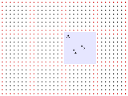
Figure 6: Example of a division of the lattice into disjoint rectangular blocks $\Lambda$ of lattice points. The subset $\partial\Lambda^{\ast}$ of points in a block $\Lambda$ with minimal distance from its boundaries (solid black lines) is referred to as the interior boundary of the block. In practice the blocks are taken to be several fm wide and normally contain many more points than shown in this sketch.

In the following, $D$ denotes the ${\rm O}(a)$-improved Wilson–Dirac operator and $S(x,y)$ the associated quark propagator on the full lattice in presence of a representative gauge field. The renormalized quark mass is assumed be positive at the chosen point in parameter space and the operator may include a twisted mass term to safely exclude accidental zero modes. The goal is then to accurately compute the propagators at source points $y$ near the center of the blocks and all $x$ at distances $|x-y|$ significantly smaller than the block edges.

On any given block $\Lambda$, let

$$D_{\Lambda}=P_{\Lambda}DP_{\Lambda},\qquad P_{\Lambda}\psi(x)=\begin{cases}\psi(x)&\hbox{if $x\in\Lambda$,}\\[2.15277pt] 0&\hbox{otherwise,}\\ \end{cases}$$ (27)

be the restriction of the Dirac operator to the block. When acting on block fields, $D_{\Lambda}$ coincides with the Dirac operator on $\Lambda$ with homogeneous Dirichlet boundary conditions. In particular, the work required for the computation of the Green function $S_{\Lambda}(x,y)$ of $D_{\Lambda}$ at all points $x\in\Lambda$ and any given source point $y\in\Lambda$ scales proportionally to the volume of $\Lambda$.

If $x$ and $y$ are not too close to the boundary of $\Lambda$, the propagator $S(x,y)$ is well approximated by the block propagator $S_{\Lambda}(x,y)$. It is possible to show this by decomposing the Wilson–Dirac operator according to

$$D=D_{b}+D_{h},\qquad D_{b}=\sum_{\Lambda}D_{\Lambda},\qquad D_{h}=\sum_{\Lambda}P_{\Lambda}D(1-P_{\Lambda}),$$ (28)

where $D_{h}$ is the sum of all hopping terms that go from one block to another. Clearly, $D_{b}$ is a sum of commuting operators and its Green function coincides with $S_{\Lambda}(x,y)$ on the block $\Lambda$. The identity

$$\frac{1}{D}-\frac{1}{D_{b}}=-\frac{1}{D_{b}}D_{h}\frac{1}{D}$$ (29)

then leads to the formula

$$S(x,y)-S_{\Lambda}(x,y)=-\sum_{z\in\partial\Lambda^{\ast}}S_{\Lambda}(x,z)(D_{h}S)(z,y),\qquad x,y\in\Lambda,$$ (30)

for the propagator difference. Recalling Eq. (26), the difference is thus seen to be exponentially suppressed with respect to $S(x,y)$ if both $x$ and $y$ are well inside the block.

5.3 Stochastic representation

Let $\eta$ be a random pseudo-fermion field with normal distribution on the interior boundaries $\partial\Lambda^{\ast}$ of the blocks $\Lambda$ (the set of points along the block boundaries in Fig. 6). Equation (30) may then be written in the form

$$S(x,y)=S_{\Lambda}(x,y)+\bigl{\langle}\phi_{\Lambda}(x)\otimes\chi(y)^{\dagger}\bigr{\rangle}_{\eta},\qquad\phi_{\Lambda}=-D_{\Lambda}^{-1}D_{h}\eta,\qquad\chi=(D^{\dagger})^{-1}\eta.$$ (31)

For each random field configuration and all points $x,y$ well inside $\Lambda$, the product of fields in the second term on the right of this formula is exponentially suppressed. A sample of a few random fields may therefore allow the term to be estimated to sufficient precision, in which case the quark propagators are obtained with a computational effort that scales proportionally to $V$ times the number of source points per block,

6 Conclusions

Master-field simulations extend the scope of numerical lattice QCD and are likely to have many interesting applications. They might sometimes be used in place of traditional simulations, where smaller lattices are simulated through large ensembles of representative fields, but whether this is profitable depends very much on the observables considered and the physics questions that are to be addressed. For computations of scattering phases for example, very large volumes are (somewhat paradoxically) not necessarily advantageous.

Apart from giving access to a new kinematic regime, master-field simulations provide a solution to the topology-freezing problem, which tends to affect lattice QCD simulations near the continuum limit. There are, however, still a few technical questions that must be addressed when the sea quarks are included in master-field simulations. In particular, global branch conditions tend to be problematic on very large lattices and should be critically reviewed. Methods based on domain decompositions and multilevel algorithms, on the other hand, are natural strategies on these lattices and are anyway recommended for reasons of algorithmic efficiency and ease of parallel processing.

In practice the memory requirements of master-field simulations can be challenging. On a $256^{4}$ lattice, for example, simulations of the SU(3) gauge theory require about $5$ TB of memory, and this figure easily rises to $100$ TB or more when the sea quarks are included in the simulations. Alternative program structures are however conceivable, where large parts of the lattice are visited in order, while the fields residing elsewhere are preserved on some storage devices other than the main memory. For reading and writing gauge-field configurations, the parallel I/O bandwidth offered by common HPC infrastructures is currently not a bottleneck.

I wish to thank the organizers of this year’s lattice conference for the kind invitation to present this work. Thanks also go to the University of Granada for hospitality at the Carmen de la Victoria, its wonderful guest house. While preparing this talk, I profited from inspiring discussions with Leonardo Giusti, and the first master-field simulations of some very large lattices could not have been completed before the conference without the help of Isabel Campos.

The simulations reported here were performed on a dedicated HPC cluster at CERN and on the FinisTerrae II machine provided by CESGA (Galicia Supercomputing Centre) to IFCA-CSIC in the framework of the H2020 project INDIGO-Datacloud (RIA 653549). FinisTerrae II was funded by the Xunta de Galicia and the Spanish MINECO under the 2007-2013 Spanish ERDF Programme. I am grateful to all these institutions for the generous support given to this work.

References

- (1) U. Wolff, Comput. Phys. Commun. 156, 143 (2004) [Erratum: ibid. 176, 383 (2007)]
- (2) K. G. Wilson, Phys. Rev. D10, 2445 (1974)
- (3) M. Lüscher, JHEP 1008, 071 (2010) [Erratum: ibid. 1403, 092 (2014)]
- (4) M. Lüscher, P. Weisz, JHEP 1102, 051 (2011)
- (5) M. Cè, C. Consonni, G.P. Engel, L. Giusti, Phys. Rev. D92, 074502 (2015)
- (6) R. Brower, S. Chandrasekharan, J.W. Negele, U.-J. Wiese, Phys. Lett. B560, 64 (2003)
- (7) S. Aoki, H. Fukaya, S. Hashimoto, T. Onogi, Phys. Rev. D76, 054508 (2007)
- (8) A. Chowdhury, A. Harindranath, J. Maiti, P. Majumdar, JHEP 1402, 045 (2014)
- (9) K.-F. Liu, J. Liang, Y.-B. Yang, arXiv:1705.06358
- (10) S. Duane, A. D. Kennedy, B. J. Pendleton, D. Roweth, Phys. Lett. B195, 216 (1987)
- (11) M. Cè, L. Giusti, S. Schaefer, Phys. Rev. D93, 094507 (2016); Phys. Rev. D95, 034503 (2017)
- (12) A. M. Horowitz, Phys. Lett. 156B, 89 (1985); Nucl. Phys. B280, 510 (1987); Phys. Lett. B268 247 (1991)
- (13) K. Jansen, C. Liu, Nucl. Phys. B453, 375 (1995) [Erratum: ibid. B459, 437 (1996)]
- (14) M. Lüscher, S. Schaefer, JHEP 1107, 036 (2011)
- (15) I. P. Omelyan, I. M. Mryglod, R. Folk, Comp. Phys. Commun. 151, 272 (2003)
-
(16)
M. Hairer, J. C. Mattingly,
Progr. Probab. 63, 109 (2011); also available at
http://www.hairer.org/papers/harris.pdf -
(17)
M. Lüscher,
unpublished notes (2017), available at
http://luscher.web.cern.ch/luscher/notes/smd-ergodicity.pdf - (18) M. Lüscher, S. Schaefer, Comput. Phys. Commun. 184, 519 (2013)
- (19) M. Dalla Brida, M. Lüscher, Eur. Phys. J. C77, 308 (2017)