Experimental entanglement of $25$ individually accessible atomic quantum interfaces

Abstract

A quantum interface links the stationary qubits in a quantum memory with flying photonic qubits in optical transmission channels and constitutes a critical element for the future quantum internet. Entanglement of quantum interfaces is an important step for the realization of quantum networks. Through heralded detection of photon interference, here we generate multipartite entanglement between $25$ (or $9$) individually addressable quantum interfaces in a multiplexed atomic quantum memory array and confirm genuine $22$ (or $9$) partite entanglement, respectively. This experimental entanglement of a record-high number of individually addressable quantum interfaces makes an important step towards the realization of quantum networks, long-distance quantum communication, and multipartite quantum information processing.

I Introduction

Stationary qubits carried by the ground states of cold atoms are an ideal memory for storage of quantum information, while flying photonic pulses are the best choice for the transmission of quantum information through the optical communication channels. A quantum interface can convert the stationary qubits into the flying photonic pulses and vice versa, and therefore generates an efficient link between the quantum memory and the optical communication channels hammerer2010quantum . A good quantum memory is provided by the hyperfine states of single atoms (ions) or the collective states of an atomic ensemble. Compared with single atoms or ions, the collective state of an atomic ensemble cannot be easily controlled for performing qubit rotations and qubit-qubit gate operations, and therefore it is not a convenient qubit for the realization of quantum computation. However, due to the collective enhancement effect, the collective state of an optically dense atomic ensemble has a unique advantage of strong coupling to the directional emission even in the free space, which generates an efficient quantum link between the atomic memory and the forward-propagating photonic pulses and hence provides an ideal candidate for the realization of the quantum interface duan2001long ; hammerer2010quantum ; kimble2008quantum . For implementation of quantum networks, long-distance quantum communication, and the future quantum internet, a promising way of scaling up is based on generating entanglement between these efficient quantum interfaces briegel1998quantum ; duan2001long ; kimble2008quantum ; hammerer2010quantum ; sangouard2011quantum ; collins2007multiplexed . Remarkable experimental advances have been reported towards this goal chou2005measurement ; chaneliere2005storage ; eisaman2005electromagnetically ; julsgaard2004experimental ; simon2007single ; de2008solid ; lan2009multiplexed ; choi2010entanglement ; saglamyurek2011broadband ; yang2016efficient ; chou2007functional . As the state of the art, up to four atomic ensemble quantum interfaces have been entangled through the heralded photon detection choi2010entanglement .

In this paper, we report a significant advance in this direction by experimentally generating multipartite entanglement between $25$, $16$, and $9$ individually addressable atomic quantum interfaces, and confirm genuine $22$, $14$, and $9$ partite entanglement respectively for these cases with a high confidence level by measuring the entanglement witness. Through programmable control and heralded detection of photon interference from a two-dimensional array of micro atomic ensembles, we generate and experimentally confirm the multipartite W-state entanglement, which is one of the most robust types of many-body entanglement and has applications in various quantum information protocols Wstate ; WT ; IonW ; haas2014entangled ; mcconnell2015entanglement . Tens to thousands of atoms in a single atomic ensemble have been entangled with a heralded photon detection haas2014entangled ; mcconnell2015entanglement . In those cases, however, the atoms are not separable or individually addressable and we do not have multipartite entanglement between individual quantum interfaces. In other experimental systems, up to $14$ ions monz201114 , $10$ photons wang2016experimental , and $10$ superconducting qubits song201710 have been prepared into genuinely entangled states. Those experiments generate multipartite entanglement between individual particles, but each particle alone cannot act as an efficient quantum interface to couple the memory qubits with the flying photons. Our experiment achieves multipartite entanglement between a record-high number of individually addressable quantum interfaces and demonstrates an important enabling step towards the realization of quantum networks, long-distance quantum communication, and multipartite quantum information processing briegel1998quantum ; duan2001long ; kimble2008quantum ; hammerer2010quantum ; sangouard2011quantum ; collins2007multiplexed ; Wstate ; WT .

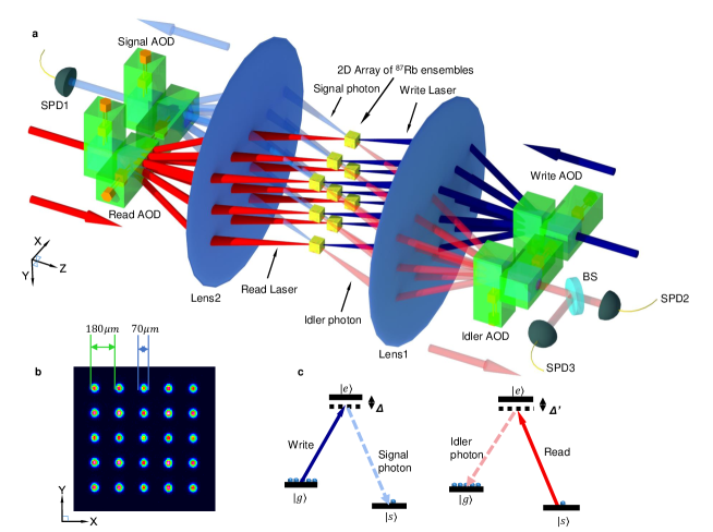
Figure 1: Experimental setup for generation and verification of multipartite entanglement between a 2D array of atomic quantum interfaces. a, We use a combination of the DLCZ scheme and the programmable AOD multiplexer to generate multipartite entanglement of the W-state type between the atomic spin waves in a 2D array of micro-ensembles. For clarity, we show a $3\times 3$ array, albeit we have also entangled $4\times 4$ and $5\times 5$ ensemble arrays. The write laser beam is split coherently into $9$ paths to simultaneously excite the $3\times 3$ ${}^{87}\mathrm{Rb}$ ensemble array by the write AOD multiplexer which contains two orthogonal deflectors placed in the X and Y directions. The lens after the AOD multiplexer focuses the beams and at the same time maps different angles of the deflected beams to different positions in a big atomic cloud forming individual micro-ensembles. The scattered signal photon modes are combined phase coherently by the lens 2 and the signal AOD de-multiplexer, and then coupled into a single-mode fiber with output detected by the single photon detector (SPD1). To verify multipartite entanglement, we use a programmable AOD multiplexer and de-multiplexer in the paths of the read beam and the idler photon mode to detect the atomic spin waves from different micro-ensembles in several complementary bases. To bound the double excitation probability, the idler photon mode is split by a 50/50 beam-splitter (BS) and detected by two single-photon detectors (SPD2 and SPD3) for registration of the three-photon coincidence (together with the SPD1). b, Illustration of the $5\times 5$ array from multiplexing of a laser beam at the position of the atomic ensemble. This image is obtained by shining a laser beam into the signal single-mode fiber which is multiplexed by the signal AOD and captured by a CCD camera at the position of atomic ensemble. The separation between adjacent signal modes is $180\,\mu$m both in X and Y directions, and the Gaussian diameter of both the signal and the idler modes is $70\,\mu$m. c, Relevant atomic energy levels and their couplings to the write/read laser beams and the signal/idler photon modes, with $|g\rangle\equiv|5S_{1/2},F=2\rangle$, $|s\rangle\equiv|5S_{1/2},F=1\rangle$, and $|e\rangle\equiv|5P_{1/2},F^{\prime}=2\rangle$. The write (read) laser beam is red detuned at $\Delta=10\,$MHz $(\Delta^{\prime}=0)$, respectively, at the center micro-ensemble.

II Results

II.1 Experimental setup

Our experimental setup is illustrated in Fig. 1. We divide a macroscopic ⁸⁷Rb atomic ensemble into a two-dimensional array of micro ensembles pu2017experimental . Each micro-ensemble is optically dense and thus can serve as an efficient quantum interface. Different micro-ensembles can be individually or collectively accessed in a programmable way through electric control of a set of cross-placed acoustic optical deflectors (AODs) lan2009multiplexed ; pu2017experimental , with details described in the Methods section. Programmable control of the experimental setup plays an important role for scalable generation of entanglement Prog .

We use a variation of the Duan-Lukin-Cirac-Zoller (DLCZ) scheme to generate multipartite entanglement between the two-dimensional array of micro atomic ensembles duan2001long . The information in each atom is carried by the hyperfine levels $|g\rangle\equiv|5S_{1/2},F=2\rangle$ and $|s\rangle\equiv|5S_{1/2},F=1\rangle$ in the ground-state manifold. All the atoms are initially prepared to the state $|g\rangle$ through optical pumping, and this initial state is denoted as $|0\rangle$ for each micro-ensemble. Through the DLCZ scheme, a weak write laser pulse can induce a Raman transition from $|g\rangle$ to $|s\rangle$, scatter a photon to the signal mode in the forward direction with an angle of $2^{\circ}$ from the write pulse, and excite a single atom into the corresponding collective spin-wave mode. This state with one collective spin-wave excitation is denoted as $|1_{i}\rangle$ for the $i$th micro-ensemble.

We generate multipartite entanglement of the W-state type between micro-ensemble quantum interfaces choi2010entanglement ; Wstate ; WT ; IonW ; haas2014entangled ; mcconnell2015entanglement . For $N$ micro-ensembles, an ideal W state has the form

$$|W_{N}\rangle=\frac{1}{\sqrt{N}}\sum_{i=1}^{N}e^{i\phi_{i}}|00\dots 1_{i}\dots 00\rangle,$$ (1)

where for the $i$th component we have a stable but adjustable phase factor $e^{i\phi_{i}}$ and a single collective spin-wave excitation in the $i$th micro-ensemble. The W state corresponds to a type of extremal multipartite entangled state most robust to the particle loss Wstate and has applications in implementation of quantum information protocols duan2001long ; kimble2008quantum ; Wstate ; WT ; IonW ; haas2014entangled ; mcconnell2015entanglement . To generate the W state entanglement between $N$ micro-ensembles, we split the write laser pulse into $N$ beams by the write AODs as shown in Fig. 1, and coherently combine the signal photon modes from $N$ micro-ensembles by the signal AODs with equal weight into a single direction which is coupled to a single-mode fiber for detection. When we register a signal photon by the detector, this photon is equally likely to come from each micro-ensemble, which has an atomic excitation in the corresponding spin-wave mode. The final state of $N$ micro-ensembles is described by the W state (1) in the ideal case as the AODs maintain coherence between different optical superposition paths.

II.2 Verification of multipartite entanglement

The experimentally prepared state differs from the ideal form (1) from contribution of several noises and imperfections. First, there is a small but nonzero probability to generate double or higher-order excitations of the photon-spin-wave pair. Second, the spin-wave mode could be in the vacuum state when we registered a photon due to the imperfect atom-photon correlation or the excitation loss in the atomic memory. Finally, even with exactly one spin-wave excitation, it may not distribute equally or perfectly coherently among $N$ micro-ensembles. The experimental state $\rho_{e}$ can be expressed as

$$\rho_{e}=p_{0}\rho_{0}+p_{1}\rho_{1}+p_{2}\rho_{2},$$ (2)

where $p_{0},p_{1},p_{2}$ and $\rho_{0},\rho_{1},\rho_{2}$ denote respectively the population and the corresponding density matrix with zero, one, and double excitations in the spin-wave modes. The state fidelity is defined as $F=\langle W_{N}|\rho_{e}|W_{N}\rangle=p_{1}\langle W_{N}|\rho_{1}|W_{N}\rangle$. In the above equation (2), we have cut the expansion to the second order excitations by neglecting tiny higher-order terms. If we assume a Poisson distribution for the number of excitations (which is the case for a parametric light-atom interaction under weak pumping), we can estimate the contribution of the higher order excitations from the measured $p_{2}/p_{1}$. Their influence turns out to be negligible to all our following results (see the supplementary materials S2 sm ).

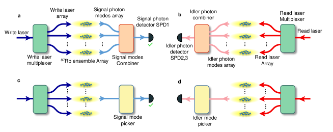
Figure 2: Programmable coupling configurations for entanglement generation and verification. a, The coupling configuration to generate multipartite entanglement, where the write AODs split the optical paths and the signal AODs coherently combine the paths. b, The detection configuration for the measurement of fidelity, where the read AODs deliver the read beams to all the micro-ensembles to transfer the atomic spin-wave excitations to idler photons and the idler AODs combine coherently the idler modes from different ensembles with equal weight for detection in the superposition basis. c,d The write and the read AODs in c and d are configured in the same way as those in a and b, but the signal and the idler AODs are programmed to successively detect the signal/idler photon from each individual micro-ensemble. The configurations c and d combined are used to calibrate the retrieval efficiency for each micro-ensemble, and the configurations a and d combined are used to detect the excitation population in each ensemble after the W state preparation (see the supplementary materials S2 for details sm ).

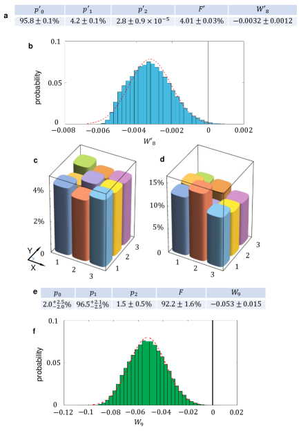
Figure 3: Entanglement verification for the $3\times 3$ array of atomic ensembles. a, The measured values, together with the $68\%$ confidence intervals (corresponding to the region within one standard deviation if the distribution is Gaussian), for the population $p^{\prime}_{0},p^{\prime}_{1},p^{\prime}_{2}$, the fidelity $F^{\prime}$, and the entanglement witness $W^{\prime}_{8}$ for the idler photon modes that are directly measured. The entanglement in the retrieved idler photon modes provides a lower bound to the entanglement in the collective spin-wave modes in different atomic ensembles. The optimized parameters in the witness $W^{\prime}_{8}$ are given by $\alpha^{\prime}_{8}=2.259\times 10^{-3}$, $\beta^{\prime}_{8}=0.7898$, and $\gamma^{\prime}_{8}=49.13$. b, The distribution of entanglement witness $W^{\prime}_{8}$, where $W^{\prime}_{8}<0$ implies 8-partite genuine entanglement. The probability with $W^{\prime}_{8}<0$ is $99.5\%$ from this measurement. c, The measured retrieval efficiency for each of the $3\times 3$ atomic ensemble array. d, The measured spin-wave excitation population in each of the $3\times 3$ atomic ensemble array after the W state preparation. e, The measured values, together with the $68\%$ confidence intervals for the population $p_{0},p_{1},p_{2}$, the fidelity $F$, and the entanglement witness $W_{9}$ for the collective spin-wave modes in different atomic ensembles after correction of the retrieval efficiency through the above measurements. The optimized parameters in the witness $W_{9}$ are given by $\alpha_{9}=0.369$, $\beta_{9}=0.889$, and $\gamma_{9}=0.268$. f, The distribution of entanglement witness $W_{9}$, where $W_{9}<0$ implies 9-partite genuine entanglement. The probability with $W_{9}<0$ is $99.98\%$ from this measurement.

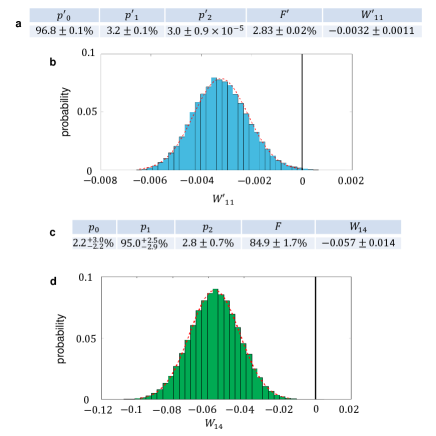
Figure 4: Entanglement verification for the $4\times 4$ array of atomic ensembles. a, The measured values, together with the $68\%$ confidence intervals, for the population $p^{\prime}_{0},p^{\prime}_{1},p^{\prime}_{2}$, the fidelity $F^{\prime}$, and the entanglement witness $W^{\prime}_{11}$, for the directly measured idler photon modes retrived from the $4\times 4$ atomic ensemble array. The optimized parameters in the witness $W^{\prime}_{11}$ are given by $\alpha^{\prime}_{11}=3.152\times 10^{-3}$, $\beta^{\prime}_{11}=0.6370$, $\gamma^{\prime}_{11}=58.14$. b, The distribution of entanglement witness $W^{\prime}_{11}$ for the $4\times 4$ idler photon modes. The probability with $W^{\prime}_{11}<0$ is $99.7\%$ from these measurements. c, The measured values, together with the $68\%$ confidence intervals, for the population $p_{0},p_{1},p_{2}$, the fidelity $F$, and the entanglement witness $W_{14}$, for the $4\times 4$ atomic ensemble array after correction of the retrieval efficiency. The optimized parameters in the witness $W_{14}$ are given by $\alpha_{14}=0.635$, $\beta_{14}=0.813$, $\gamma_{14}=0.240$. d, The distribution of entanglement witness $W_{14}$ for the $4\times 4$ case. The probability with $W_{14}<0$ is $99.997\%$ from these measurements.

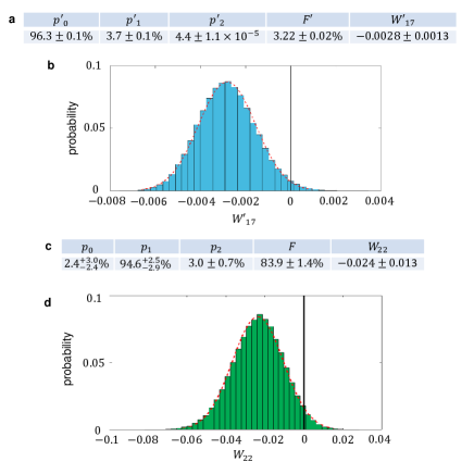
Figure 5: Entanglement verification for the $5\times 5$ array of atomic ensembles. a, The measured values, together with the $68\%$ confidence intervals, for the population $p^{\prime}_{0},p^{\prime}_{1},p^{\prime}_{2}$, the fidelity $F^{\prime}$, and the entanglement witness $W^{\prime}_{17}$, for the directly measured idler photon modes retrieved from the $5\times 5$ atomic ensemble array. The optimized parameters in the witness $W^{\prime}_{17}$ are given by $\alpha^{\prime}_{17}=3.317\times 10^{-3}$, $\beta^{\prime}_{17}=0.6516$, $\gamma^{\prime}_{17}=53.65$. b, The distribution of entanglement witness $W^{\prime}_{17}$ for the $5\times 5$ idler photon modes. The probability with $W^{\prime}_{17}<0$ is $98.4\%$ from these measurements. c, The measured values, together with the $68\%$ confidence intervals, for the population $p_{0},p_{1},p_{2}$, the fidelity $F$, and the entanglement witness $W_{22}$, for the $5\times 5$ atomic ensemble array after correction of the retrieval efficiency. The optimized parameters in the witness $W_{22}$ are given by $\alpha_{22}=0.550$, $\beta_{22}=0.840$, $\gamma_{22}=0.244$. d, The distribution of entanglement witness $W_{22}$ for the $5\times 5$ case. The probability with $W_{22}<0$ is $96.5\%$ from these measurements.

To verify multipartite quantum entanglement between $N$ quantum interfaces, we use entanglement witness to lower bound the entanglement depth $k$ ($k\leq N$) EDepth , which means the state $\rho_{e}$ has at least $k$-partite genuine quantum entanglement guhne2009entanglement . An entanglement witness appropriate for the W-type entangled state is given by $\mathcal{W}_{k}=\alpha_{k}P_{0}+\beta_{k}P_{1}+\gamma_{k}P_{2}-|W_{N}\rangle\langle W_{N}|$ guhne2009entanglement , where $P_{n}$ ($n=0,1,2$) denote the projectors onto the subspace with $n$ excitations in the spin-wave modes and the parameters $\alpha_{k},\beta_{k},\gamma_{k}\geq 0$ are numerically optimized (see the supplementary materials S1 sm ) such that for any state $\rho_{a}$ with entanglement depth less than $k$, the witness is non-negative, i.e. $\mathrm{tr}[\mathcal{W}_{k}\rho_{a}]=\alpha_{k}p_{0}+\beta_{k}p_{1}+\gamma_{k}p_{2}-F\geq 0$. Therefore, $\mathrm{tr}[\mathcal{W}_{k}\rho_{e}]<0$ serves as a sufficient condition to verify that we have at least $k$-partite genuine entanglement among the $N$ quantum interfaces. Note that this witness does not require $p_{0}+p_{1}+p_{2}=1$, so it also applies in the case with $p_{0}+p_{1}+p_{2}<1$ when we consider small higher-order excitations, although the corrections turn out to be negligible for all our following results sm ).

To bound the entanglement depth, we experimentally measure the fidelity $F$ and the population $p_{0},p_{1},p_{2}$. The detailed measurement procedure is explained in the supplementary materials S2 sm . The spin-wave excitation in each quantum interface is retrieved to the idler photon for detection by a read laser beam. Our measurement is directly on the state of the retrieved photon, which can be represented by a form similar to equation (2) for the spin-wave modes. Due to the limited retrieval efficiency, detector inefficiency, and the associated photon loss, the detected idler photon modes have much larger vacuum components, and their corresponding parameters are denoted as $F^{\prime}$ and $p^{\prime}_{0},p^{\prime}_{1},p^{\prime}_{2}$. Because this retrieval process is a local operation, the entanglement in the retrieved photonic modes provides a lower bound to the entanglement in the collective spin-wave modes in the atomic ensembles choi2010entanglement .

The fidelity $F^{\prime}$ and the populations $p^{\prime}_{0},p^{\prime}_{1},p^{\prime}_{2}$ of the idler photon are determined in the following way. We first measure the double excitation probability $p^{\prime}_{2}$ from the photon intensity correlation of the two single photon detectors in the idler modes, conditioned on a photon click in the signal mode. Then $p^{\prime}_{1},p^{\prime}_{0}$ and $F^{\prime}$ are measured by programming the four sets (write, signal, read, and idler) of AODs in different configurations as shown in Fig. 2 (see details in the supplementary materials S2 and figures S1-S4 there sm ). When we measure the population $p^{\prime}_{1}$, the idler AOD successively picks up the output photon mode of each individual micro-ensemble for detection; and as for the fidelity $F^{\prime}$, the idler AOD coherently combines the output idler modes from the $N$ micro-ensembles with equal weight to the single-mode fiber for detection, which gives an effective projection to the state $|W_{N}\rangle$. Note that the fidelity measurement is sensitive to the relative phase information between different idler photon modes as these modes interfere at the AODs through the coherent combination. After $F^{\prime}$ and $p^{\prime}_{0},p^{\prime}_{1},p^{\prime}_{2}$ are measured, we calibrate the retrieval efficiency for each micro-ensemble, and finally derive the fidelity $F$ and populations $p_{0},p_{1},p_{2}$ of the spin-wave modes from the measured idler photon statistics Chou2004 . The detailed conversion procedure is described in the supplementary materials S2 sm .

We have performed the entanglement preparation and verification experiments with $3\times 3$, $4\times 4$ and $5\times 5$ arrays of micro-ensembles. For $9$ individually addressable micro-ensembles, the results are shown in Fig. 3. We present the parameters for the idler photon state in Fig. 3a, and the probability to have $8$-partite entanglement is $99.5\%$ for the photon state. After conversion with the calibrated retrieval efficiency, we find that the state of the atomic micro-ensembles has a high fidelity of $F=(92.2\pm 1.6)\%$ to be in the $9$-partite W state. In Fig. 3d, we show the distribution of the entanglement witness $W_{9}=\mathrm{tr}[\mathcal{W}_{9}\rho_{e}]$ from the experimental data. From this distribution, we conclude with a confidence level of $99.98\%$ that we have generated genuine $9$-partite quantum entanglement among the $9$ atomic ensembles.

In Fig. 4 and Fig. 5, we show the experimental results for $16$ and $25$ micro-ensembles. In these cases, the fidelity is not high enough to prove all of them are genuinely entangled. The calibrated fidelities $F$ for the atomic states are $(84.9\pm 1.7)\%$ and $(83.9\pm 1.4)\%$, respectively. With more ensembles, it becomes harder to maintain the uniformity in the optical depth and the laser excitation probability for each ensemble, which causes the fidelity to decay. However, we can still use the entanglement witness to demonstrate a high entanglement depth. As shown in Fig. 4 and Fig. 5, for $16$ ensembles, we have confirmed $11$-partite entanglement in the retrieved idler photon modes with a confidence level of $99.7\%$ and $14$-partite entanglement between the spin-wave modes in the $16$ micro-ensembles with a confidence level of $99.997\%$ after correction with the calibrated retrieval efficiency; and for $25$ ensembles, we have confirmed $17$-partite entanglement in the retrieved photonic modes with a confidence level of $98.4\%$ and $22$-partite entanglement between the $25$ micro-ensembles with a confidence level of $96.5\%$.

III Discussion

Our experimental preparation of multipartite entanglement in a record-high number of individually addressable quantum interfaces represents a significant milestone in quantum state engineering. Through programming of AODs to control intrinsically stable optical interference paths, the entanglement preparation and verification techniques developed in this experiment are fully scalable to a larger number of quantum interfaces. It is feasible to use AODs to program and direct the focused laser beams to hundreds of micro-ensembles pu2017experimental . The number of entangled ensembles in our current experiment is basically limited by the size of the whole atomic cloud and the available optical depth. With the use of double magneto-optical traps for more efficient atom loading, we can significantly increase the size of the atomic cloud, the optical depth, and the retrieval efficiency for the stored photons. In that case, we should be able to get hundreds of micro-ensembles entangled by the same control setup and entanglement verification techniques reported in this experiment. Generation of multipartite entanglement between many individually addressable quantum interfaces demonstrates an important step towards the realization of quantum networks kimble2008quantum ; duan2001long , long-distance quantum communication duan2001long ; briegel1998quantum ; sangouard2011quantum , and multipartite quantum information processing kimble2008quantum ; choi2010entanglement ; Wstate ; WT .

Note Added. After post of this work to arxiv (arXiv:1707.09701), we became aware of related independent works in Refs. Simon2017 ; Gisin2017 , which report generation of multi-particle W state entanglement in solid-state ensembles. Compared with those experiments, we realized multipartite entanglement between spatially separated micro-ensembles of neutral atoms which are individually accessible by focused laser beams with programmable control of the AODs. We thank C. Simon for bringing Refs. Simon2017 ; Gisin2017 to our attention.

Materials and Methods

Experimental methods. A ⁸⁷Rb atomic cloud is loaded into a magneto-optical trap (MOT). For cooling and trapping of the atoms in the MOT, a strong cooling beam, red detuned to the D2 cycling transition $|g\rangle\equiv|5S_{1/2},F=2\rangle\rightarrow|5P_{3/2},F=3\rangle$ by $12\,$MHz, is used. The repumping laser, resonant to the $|s\rangle\equiv|5S_{1/2},F=1\rangle\rightarrow|5P_{3/2},F=2\rangle$ transition, pumps back those atoms which fall out of the cooling transition. The temperature of the atoms is about $300\,\mu$K in the MOT. The atoms are then further cooled by polarization gradient cooling (PGC) for $1\,$ms. The PGC is implemented by increasing the red detuning of the cooling laser to $60\,$MHz, and reducing the intensity to half of the value at the MOT loading stage. At the same time, the repumping laser intensity is decreased to $0.5\%$ of the value at the loading phase, and the magnetic gradient coil is shut off. The temperature is reduced to about $30\,\mu$K after this process and the size of the MOT remains almost the same. After the PGC some atoms are scattered to the $|s\rangle$ state, and we use a $100\,\mu$s repumping pulse to pump all the atoms back to $|g\rangle$. During the storage, the ambient magnetic field is not compensated, so the retrieval efficiency of the collective spin-wave excitation undergoes Larmor precession. In our case, the Larmor period is $5.8\,\mu$s. The time interval between the read and the write pulses is set to this Larmor period to achieve the highest retrieval efficiency for the idler photon.

The experimental sequence begins with a write pulse of $100\,$ns long, which is split by the write AODs to $N$ paths to excite the two-dimensional (2D) array of atomic ensembles. If no signal photon is detected, a clearance pulse identical to the read pulse will pump the atoms back to $|g\rangle$. The write-clearance sequence is repeated until a signal photon is detected. Upon detection of the signal photon, the corresponding collective spin-wave excitation is stored in the atomic ensemble for a controllable period of time and then retrieved by a read pulse to a photon in the idler mode. The conditional control of write/read pulses is implemented by a field-programmable gate array (FPGA). The signal or idler photons collected by the single-mode optical fiber are directed to a single-photon counting module (SPCM). The photon countings and their coincidence are registered through the FPGA.

Control of acoustic optical deflectors. The radio-frequency (RF) signal is generated by two $4$-channel arbitrary-waveform generators (AWG, Tektronix 5014C). One of the AWG supplies the RF for write, read, signal, and idler acoustic optical deflectors (AODs, AA DTSXY-400) in the $X$ direction, and the other supplies the RF for the AODs in the $Y$ direction. The outputs of the AWG channels are amplified by a $2\,$W RF amplifier (Mini-circuits, ZHL-1-2W) to drive the AODs.

The nonlinearity in the amplifier and the AODs could induce other unwanted frequency components, which cause imperfections in the mode multiplexing and de-multiplexing. By carefully tuning the relative phases in read, signal, and idler AODs as discussed in endres2016atom , we can attenuate the influence from these unwanted frequency components by an extinction ratio about $120\,$dB, which becomes negligible for our experiment.

Although the AODs split the optical paths into many different branches, the relative optical phases between different branches are intrinsically stable as different optical paths in our experiment go through the same optics elements. This is an important advantage which eliminates the need of complicated active phase stabilization for many optical interferometer loops in our experiment. The relative phases between different superposition paths are adjusted in experiments by controlling the phases of different RF frequency components that drive the write AODs.

Acknowledgements We thank A. Kuzmich and Y.-M. Liu for discussions. This work was supported by the Ministry of Education of China and the Tsinghua-QTEC Joint Lab on quantum networks. LMD acknowledges in addition support from the ARL CDQI program.

Author Contributions L.M.D. conceived the experiment and supervised the project. Y.F.P., N.J., W.C., C.L., S.Z. carried out the experiment. Y.K.W. optimized the entanglement witness. L.M.D., Y.F.P., Y.K.W. wrote the manuscript.

Author Information The authors declare no competing financial interests. Correspondence and requests for materials should be addressed to L.M.D. (lmduan@umich.edu).

Data and materials availability: All data needed to evaluate the conclusions in the paper are present in the paper and/or the Supplementary Materials. Additional data related to this paper may be requested from the authors.

Supplementary text

IV Section S1. Entanglement witness for W-type states

Ideally, we should generate the W-type multipartite entangled states. Due to noise and imperfections, the experimentally prepared state is always mixed. To verify multipartite entanglement in the proximity of the W states, we use the following entanglement witness introduced in Ref. guhne2009entanglement

$$\mathcal{W}_{k}=\alpha_{k}P_{0}+\beta_{k}P_{1}+\gamma_{k}P_{2}-|W_{N}\rangle\langle W_{N}|,$$ (3)

where $P_{n}$ ($n=0,1,2$) is the projector onto the subspace with $n$ excitations ($n$ ($n\leq N$) qubits in the $\left|1\right\rangle$ state), and

$$|W_{N}\rangle=\frac{1}{\sqrt{N}}\left(|10\cdots 00\rangle+|01\cdots 00\rangle+\dots+|00\cdots 01\rangle\right)$$ (4)

denotes the $N$-qubit W state, where we have neglected the unimportant relative phases between the superposition terms as they can be absorbed into the definition of the basis states. The parameters $\alpha_{k},\beta_{k},\gamma_{k}\geq 0$ are chosen such that for any state $\rho$ with entanglement depth $E_{d}$ less than $k$ (states without genuine $k$-partite entanglement), the witness is non-negative, i.e., $\mathrm{tr}(\mathcal{W}_{k}\rho)\geq 0$.

In the following, we briefly describe how to optimize this entanglement witness following the derivation given in Ref. Guhne2009, which is referred to for the full details of the arguments. We pay particular attention to optimizing the parameters $\alpha_{k},\beta_{k},\gamma_{k}$ for our experimental configurations. Since a general density operator $\rho$ can always be expressed as a convex combination of pure states, it suffices to consider the non-negativity over pure states $|\phi\rangle$ with $E_{d}<k$. Furthermore, due to the permutation symmetry of the W state and the $P_{n}$ operators, we can write $|\phi\rangle=|a\rangle_{1,\cdots,l}|b\rangle_{l+1,\cdots,N}$ ($l,N-l\leq k$) without loss of generality. Here we are mainly interested in the case where $k$ is close to $N$ and hence we assume $k\geq 2N/3$. The above expression also includes the case where $|\phi\rangle$ can be separated into the tensor product of more than two parts. If we find such an entanglement witness $\mathcal{W}_{k}$ characterized by the parameters $\alpha_{k}$, $\beta_{k}$, $\gamma_{k}$, and if the experimentally generated state $\rho_{e}$ satisfies $\mathrm{tr}(\mathcal{W}_{k}\rho_{e})=\alpha_{k}p_{0}+\beta_{k}p_{1}+\gamma_{k}p_{2}-F<0$, we can conclude that the state $\rho_{e}$ must possess at least genuine $k$-partite entanglement. The parameters $p_{0},p_{1},p_{2}$ in the above witness denote the population with zero, one, or double excitations in the spin-wave modes and $F\equiv\langle W_{N}|\rho_{e}|W_{N}\rangle$ denotes the state fidelity. The parameters $p_{0},p_{1},p_{2},F$ are directly measured in our experiment.

The component state $|a\rangle_{1,\cdots,l}$ (and similarly $|b\rangle_{l+1,\cdots,N}$) can be generally expanded as

$$|a\rangle_{1,\cdots,l}=a_{0}|g\rangle_{1,\cdots,l}+a_{1}|e_{1}\rangle_{1,\cdots,l}+\cdots+a_{l}|e_{l}\rangle_{1,\cdots,l}$$ (5)

where $|g\rangle_{1,\cdots,l}=|00\cdots 0\rangle_{1,\cdots,l}$ denotes the ground state with all the qubits in the $|0\rangle$ state, $|e_{1}\rangle_{1,\cdots,l}\propto P_{1}|a\rangle_{1,\cdots,l}$ is a normalized state with exactly one excitation, and $|e_{l}\rangle_{1,\cdots,l}$ denotes a state with exactly $l$ excitations. Our purpose is to find out the optimal parameters $\alpha_{k},\beta_{k},\gamma_{k}$ so that for any state $|\phi\rangle$ with above decomposition, we have $\mathrm{tr}(\mathcal{W}_{k}|\phi\rangle\langle\phi|)\geq 0$. The non-negativity of the witness is not affected by normalization of the state. Suppose we have a state $|\phi\rangle=(a_{0}|g\rangle+a_{1}|e_{1}\rangle)_{1,\cdots,l}(b_{0}|g^{\prime}\rangle+b_{1}|e_{1}^{\prime}\rangle)_{l+1,\cdots,N}$ whose witness is non-negative, i.e., $\mathrm{tr}(\mathcal{W}_{k}|\phi\rangle\langle\phi|)\geq 0$. Now if we keep $a_{0}$, $a_{1}$, $b_{0}$ and $b_{1}$ unchanged but introduce non-zero $a_{2},\cdots,a_{l},b_{2},\cdots,b_{N-l}$ terms, the projection onto $P_{0}$, $P_{1}$ and $|W_{N}\rangle\langle W_{N}|$ remain unaffected while the projection on $P_{2}$ may increase, because the added terms have at least two excitations. Therefore this new state is guaranteed to have a non-negative witness. In other words, to test the non-negativity of the entanglement witness, we only need to consider bi-decomposable pure states $|\phi\rangle$ with each part staying in the subspace of no more than one excitation. For the same reason, only the completely symmetric state $|W_{l}\rangle$ ($|W_{N-l}\rangle$) needs to be considered in the one-excitation subspace, since a one-excitation state orthogonal to the symmetric state is also orthogonal to $|W_{N}\rangle$ but still contributes to the $P_{1}$ and $P_{2}$ terms.

Through the above reasoning, we only need to find optimal $\alpha_{k},\beta_{k},\gamma_{k}$ such that for any $l,N-l\leq k$ and any complex numbers $a_{0},a_{1},b_{0},b_{1}$ with $|a_{0}|^{2}+|a_{1}|^{2}=|b_{0}|^{2}+|b_{1}|^{2}=1$, the state

$$|\phi\rangle=(a_{0}|g\rangle+a_{1}|W_{l}\rangle)_{1,\cdots,l}(b_{0}|g^{\prime}\rangle+b_{1}|W_{N-l}\rangle)_{l+1,\cdots,N}$$ (6)

has non-negative witness $\mathrm{tr}(\mathcal{W}_{k}|\phi\rangle\langle\phi|)\equiv f\geq 0$, which can be expressed as

$$f = \alpha_{k}|a_{0}|^{2}|b_{0}|^{2}+\beta_{k}(|a_{0}|^{2}|b_{1}|^{2}+|a_{1}|^{2}|b_{0}|^{2})$$

$$+\gamma_{k}|a_{1}|^{2}|b_{1}|^{2}-\frac{1}{N}\left|\sqrt{N-l}a_{0}b_{1}+\sqrt{l}a_{1}b_{0}\right|^{2}.$$

The parameters $\alpha_{k},\beta_{k},\gamma_{k}$ should be chosen such that the minimal value of $f$ is non-negative. Clearly this function is minimized when $a_{0}$, $a_{1}$, $b_{0}$ and $b_{1}$ are in phase, so we can choose $0\leq a_{0},a_{1},b_{0},b_{1}\leq 1$. Therefore, we can express them as $a_{0}=\cos\theta_{1}$, $a_{1}=\sin\theta_{1}$, $b_{0}=\cos\theta_{2}$, $b_{1}=\sin\theta_{2}$ ($0\leq\theta_{1},\theta_{2}\leq\pi/2$). With the new parameters $\theta_{1},\theta_{2}$, we have

$$f= \frac{1}{4}\bigg{[}\alpha_{k}(1+\cos 2\theta_{1})(1+\cos 2\theta_{2})+2\beta_{k}(1-\cos 2\theta_{1}\cos 2\theta_{2})$$

$$+\gamma_{k}(1-\cos 2\theta_{1})(1-\cos 2\theta_{2})-(1+\cos 2\theta_{1})(1-\cos 2\theta_{2})$$

$$+\frac{2l}{N}(\cos 2\theta_{1}-\cos 2\theta_{2})-\frac{2\sqrt{l(N-l)}}{N}\sin 2\theta_{1}\sin 2\theta_{2}\bigg{]}.$$ (8)

To find the minimum of this objective function, we calculate the partial derivatives $\partial f/\partial\theta_{1}$ and $\partial f/\partial\theta_{2}$ with respect to $\theta_{1}$ and $\theta_{2}$. Inside the rectangular region $(0,\pi/2)\times(0,\pi/2)$, stationary points are determined by $\partial f/\partial\theta_{1}=\partial f/\partial\theta_{2}=0$, which gives,

$$\tan 2\theta_{1}= \frac{\frac{2\sqrt{l(N-l)}}{N}\sin 2\theta_{2}}{-\alpha_{k}(1+\cos 2\theta_{2})+2\beta_{k}\cos 2\theta_{2}+\gamma_{k}(1-\cos 2\theta_{2})+(1-\cos 2\theta_{2})-\frac{2l}{N}},$$ (9)

$$\tan 2\theta_{2}= \frac{\frac{2\sqrt{l(N-l)}}{N}\sin 2\theta_{1}}{-\alpha_{k}(1+\cos 2\theta_{1})+2\beta_{k}\cos 2\theta_{1}+\gamma_{k}(1-\cos 2\theta_{1})-(1+\cos 2\theta_{1})+\frac{2l}{N}}.$$ (10)

To find the stationary point solution, we choose an arbitrary initial point inside the region, say, with $\theta_{1}=\theta_{2}=\pi/4$, and then apply the substitution Eq. (9) and Eq. (10) iteratively until the result converges. With this method, we get the minimum of $f$ with respect to $\theta_{1},\theta_{2}$ for a given $l$. This minimum of $f$ is also compared with the value of $f$ at the boundary to get the absolute minimum of $f$ in the rectangular region. Finally, the integer parameter $l$ is scanned so that we get the absolute minimum of $f$, denoted as $f_{m}$, with respect to the parameters $l,\theta_{1},\theta_{2}$.

We choose the parameters $\alpha_{k},\beta_{k},\gamma_{k}$ so that the witness condition $f_{m}\geq 0$ is satisfied. There are infinite combinations of $\alpha_{k},\beta_{k},\gamma_{k}$ that satisfy this requirement. To find the optimal $\alpha_{k},\beta_{k},\gamma_{k}$ for given experimental data $p_{0},p_{1},p_{2},F$, we choose a combination of $\alpha_{k},\beta_{k},\gamma_{k}$ that leads to the smallest (most negative) entanglement witness $\mathrm{tr}(\mathcal{W}_{k}\rho_{e})=\alpha_{k}p_{0}+\beta_{k}p_{1}+\gamma_{k}p_{2}-F$ because it is the negative value of the witness $\mathrm{tr}(\mathcal{W}_{k}\rho_{e})$ that indicates the existence of $k$-partite entanglement. The parameters $\alpha_{k},\beta_{k},\gamma_{k}$ in the caption of Figs. 3 and 4 are determined in this way for verification of genuine multipartite entanglement with $k=9,14,22$ and $N=9,16,25$, respectively. For measurement of the retrieved idler photon modes, $\alpha^{\prime}_{k},\beta^{\prime}_{k},\gamma^{\prime}_{k}$ are optimized for the measured $p^{\prime}_{0},p^{\prime}_{1},p^{\prime}_{2},F^{\prime}$ in a similar way.

Note that although we assume a truncated number of excitations in the atomic micro-ensembles, as is shown in Eq. (2) in the main text, the entanglement witness we use here is exact. The above derivation actually allows the existence of higher order excitations by simply taking $p_{0}+p_{1}+p_{2}<1$. Later we will bound the effects of higher order excitations on the measured probabilities and therefore give a lower-bound on the entanglement depth.

V Section S2. Experimental measurement of the entanglement witness

To experimentally verify multipartite entanglement, we measure the entanglement witness $\mathrm{tr}(\mathcal{W}_{k}\rho_{e})=\alpha_{k}p_{0}+\beta_{k}p_{1}+\gamma_{k}p_{2}-F$, which reduces to measurements of four parameters $p_{0},p_{1},p_{2},F$. To measure these parameters for the spin-wave states in the atomic ensembles, all the detections are done through the conversion of spin-wave excitations to the idler photons. First, we need to calibrate the retrieval efficiency $\eta_{i}$ for each micro-ensemble, which is defined as the probability to register a photon count in the idler mode by the single-photon detector given a single excitation in the corresponding collective spin-wave mode.

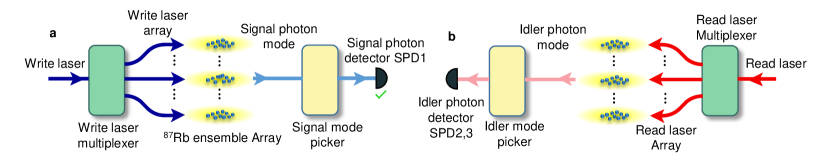
Figure 6: Coupling configuration for the measurement of the retrieval efficiency of each micro-ensemble. a, The write AODs coherently split the write beam into $N$ paths to excite all the micro-ensembles simultaneously, and the signal AODs are programmed to detect the signal photon from one of the $N$ micro-ensembles. The detection of a signal photon by SPD1 heralds the generation of an atomic spin-wave excitation in the corresponding micro-ensemble. b, The read AODs deliver the read beam to transfer all the atomic spin-wave excitations to idler photons, and the idler AODs are programmed to detect the idler photon from the same micro-ensemble where the signal photon is detected in a.

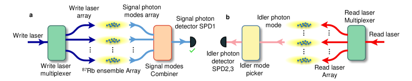
Figure 7: Coupling configuration for the measurement of the excitation population of each micro-ensemble. a, The write AODs split the optical paths and the signal AODs coherently combine the paths. The generation of a spin-wave W state is heralded by the detection of a photon in the combined signal mode. b, The read AODs coherently split the read beam to transfer all the atomic spin-wave excitations to idler photons, and the idler AODs are programmed to detect the idler photon from one of the $N$ micro-ensembles to measure its excitation population.

Figure 8: Coupling configuration for the measurement of the $W$ state fidelity. a, The write AODs coherently split the optical paths and the signal AODs coherently combine the paths. The generation of a spin-wave W state is heralded by the detection of a photon in the combined signal mode. b, The read AODs coherently split the read beams to all the micro-ensembles to transfer the atomic spin-wave excitations to idler photons and the idler AODs coherently combine the idler modes from different micro-ensembles with equal weight for the detection in the superposition basis.

We measure the retrieval efficiency by the setup shown in Fig. S1. Through control of the AODs, we successively excite and measure each micro-ensemble through the standard DLCZ scheme. For the $i$th ensemble, through the measured photon counts on the signal and idler modes and their coincidence, we get the probability $P_{S}^{(i)}$ ($P_{I}^{(i)}$) to record a photon count in the signal (idler) mode in each experimental trial and the joint probability $P_{SI}^{(i)}$ to detect a coincidence. The coincidence probability can be expressed as

$$P_{SI}^{(i)}=\eta_{i}P_{S}^{(i)}+P_{S}^{(i)}P_{I}^{(i)},$$ (11)

where the second term $P_{S}^{(i)}P_{I}^{(i)}$ denotes the random coincidence from two independent distributions and the first term denotes the retrieved signal with the retrieval efficiency $\eta_{i}$. From the above expression, we get $\eta_{i}=P_{SI}^{(i)}/P_{S}^{(i)}-P_{I}^{(i)}$, which is inferred from the three measured qualities $P_{S}^{(i)},P_{I}^{(i)},P_{SI}^{(i)}$. For our experiment, the measured retrieval efficiencies are close to $4\%$ for all the micro-ensembles. For the $3\times 3$ micro-ensemble array, the results of the measured $\eta_{i}$ are shown in Fig. 3c of the main text.

After determination of the retrieval efficiency $\eta_{i}$, we can then measure the population $p_{0},p_{1},p_{2}$ and the fidelity $F$. In our experiment, the double excitation probability $p_{2}$ is quite small. To illustrate the basic idea of detection method, first we look at a simple case by neglecting the contribution of $p_{2}$ (later we will go to the more realistic case by determining the small but nonzero $p_{2}$). Without the contribution of $p_{2}$, the experimental density matrix has the simplified form $\rho_{e}=p_{0}\rho_{0}+p_{1}\rho_{1}$. To measure $p_{1}$, we use the setup shown in Fig. S2. After preparation of the state with the excitation configuration in Fig. S2a, we successively pick up the idler mode from each micro-ensemble to measure the photon counts as shown in Fig. S2b. The measured probability $q_{i}$ to record a photon count from the $i$th idler mode in each experimental trial is given by

$$q_{i}=\eta_{i}p_{1}\langle i|\rho_{1}|i\rangle,$$ (12)

where $|i\rangle\equiv|00\dots 1_{i}\dots 00\rangle$ denotes the state with a spin-wave excitation in the $i^{th}$ micro-ensemble and none in others. From this expression, we get $\sum_{i}$ $q_{i}/\eta_{i}=p_{1}\sum_{i}\langle i|\rho_{1}|i\rangle=p_{1}$, so we obtain $p_{1}$ and $p_{0}=1-p_{1}$ from the measured $q_{i}$ and $\eta_{i}$. As an example, for the case of $3\times 3$ micro-ensemble array, the results of the measured $q_{i}/\eta_{i}$ are shown in Fig. 3d of the main text. Meanwhile, we can measure the idler photonic single-excitation population by not correcting the retrieval efficiency, that is, $p^{\prime}_{1}=\sum q_{i}$, which is just the sum of the measured probabilities in each of the $N$ modes.

For this simple case, it is also easy to determine the fidelity $F$, which is measured by the setup shown in Fig. S3. In Fig. S3b, the idler AODs are set to equally and coherently combine the idler modes from all the $N$ micro-ensembles. If we neglect the small inhomogeneity in the retrieval efficiencies $\eta_{i}$ and replace $\eta_{i}$ with their average $\overline{\eta}$, the measured probability $q_{f}$ to record a photon count from the combined mode in Fig. S3b in each experimental trial is just given by $q_{f}=\overline{\eta}\langle W_{N}|\rho_{e}|W_{N}\rangle=\overline{\eta}F$, which gives the fidelity as $F=q_{f}/\overline{\eta}$ from the measured quantities $q_{f}$ and $\overline{\eta}$. Later we will take into account both the contributions of the double excitation probability $p_{2}$ and the inhomogeneity in $\eta_{i}$ to correct the formula for the fidelity $F$. The photonic fidelity $F^{\prime}=q_{f}$ is just the measured probability of detector in this fidelity measurement setup.

Now we consider the contribution of the double excitation probability $p_{2}$. First we need to measure this small probability $p_{2}$ in our experiment. The measurement configuration is shown by the supplementary Fig. S4, where we split the combined idler photon mode by a 50/50 beam splitter and detect the three-photon coincidence between the single photon detectors D1, D2, and D3. We measure the normalized three-photon correlation, defined by

$$\alpha\equiv\frac{q_{1}q_{123}}{q_{12}q_{13}},$$ (13)

where $q_{1},q_{12},q_{13},q_{123}$ denote respectively the probabilities of registering a photon count on detector 1, a coincidence of counts between detectors 1 and 2, a coincidence between detectors 1 and 3, and a coincidence between detectors 1, 2 and 3 in each experimental trial. By this definition, $\alpha$ becomes independent of the detector efficiency and the transfer efficiency from the spin-wave modes to the photon modes as their contributions to the numerator and the denominator of $\alpha$ cancel with each other. The normalized correlation is thus given by

$$\alpha=\frac{p_{2}\langle 0|a_{W}^{2}\rho_{2}a_{W}^{{\dagger}2}|0\rangle}{p_{1}^{2}|\langle 0|a_{W}\rho_{1}a_{W}^{{\dagger}}|0\rangle|^{2}},$$ (14)

where $a_{W}$ ($a_{W}^{{\dagger}}$) denotes the annihilation (creation) operator for the spin-wave modes in the W state.

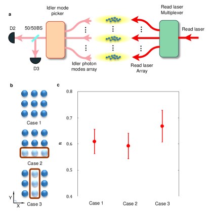
Figure 9: Measurement of the three-photon correlation and the double excitation probability. a, The detection configuration for measurement of the double excitation probability $p_{2}$, where a 50/50 beam splitter is inserted to split the combined idler mode to detect the double excitations in this mode. We combine this detection configuration with the entanglement generation configuration shown in Fig. S3a, where the detector D1 registers a signal photon in the combined mode. We register the three-photon coincidence between the detectors D1, D2, and D3, and from it construct the normalized three-photon correlation $\alpha$ and the double excitation probability $p_{2}$ as explained in the supplementary text. b,c Test of the three-photon correlation $\alpha$ under different measurement bases. We check three arbitrarily chosen bases here. In case 1, we detect in the full superposition basis from the $3\times 3$ ensemble array. In case 2 and 3, we detect in the partial superposition basis from the $2\times 3$ (1st and 2nd rows) and $3\times 2$ (1st and 3rd columns) ensemble arrays, respectively, as illustrated in b. The measured three-photon correlations $\alpha$ shown in c are independent of the measurement bases within the experimental error bar (the error bar corresponds to one standard deviation). Note that for the test measurement shown in c we have increased the write laser intensity compared with the one for the W state generation to get a higher three-photon coincidence rate, so the value of $\alpha$ is also higher than what we have for the W state preparation experiment.

From our excitation configuration for preparation of the W state, the dominant excitations in $\rho_{1}$ and $\rho_{2}$ should be along the same spin-wave mode as they come from the driving by the same write beam. Neglecting small imperfection terms, we can express $\rho_{1}$ and $\rho_{2}$ approximately as

$$\rho_{1}\approx a_{e}^{{\dagger}}\rho_{0}a_{e},\text{ }\rho_{2}\approx a_{e}^{{\dagger}2}\rho_{0}a_{e}^{2}/2,$$ (15)

where $\rho_{0}$ denotes the vacuum for spin-wave excitations and $a_{e}$ denotes the excited spin-wave mode, which in our experiment is quite close to the mode $a_{W}$ for the W state. The factor of $1/2$ in $\rho_{2}$ comes from normalization $tr(\rho_{2})=1$. Under this approximation, we have $\langle 0|a_{W}^{2}\rho_{2}a_{W}^{{\dagger}2}|0\rangle\approx 2\left|[a_{W},a_{e}^{{\dagger}}]\right|^{4}$, $\langle 0|a_{W}\rho_{1}a_{W}^{{\dagger}}|0\rangle\approx\left|[a_{W},a_{e}^{{\dagger}}]\right|^{2}$. So the normalized correlation reduces to

$$\alpha\approx\frac{2p_{2}}{p_{1}^{2}}.$$ (16)

By measuring the normalized correlation $\alpha$, we thus get a simple relation between the double-excitation and single-excitation probabilities $p_{2}$ and $p_{1}$. (As $\alpha$ is a normalized quantity, independent of the retrieval efficiency and the photon loss, for the directly measured idler photon modes, we still have $\alpha=2p^{\prime}_{2}/{(p^{\prime}_{1})^{2}}$. As $p^{\prime}_{1}=2q_{12}/q_{1}=2q_{13}/q_{1}$, from the definition of $\alpha$, we then have $p^{\prime}_{2}=2q_{123}/q_{1}$, which is consistent to what we expect from the definition of the coincidence counts. In analyzing the experimental data, we use the formula $p^{\prime}_{2}=\alpha({p^{\prime}_{1}})^{2}/2$ to derive $p^{\prime}_{2}$ from the measured $\alpha$ and $p^{\prime}_{1}$, and then deduce $p^{\prime}_{0}$ by $p^{\prime}_{0}=1-p^{\prime}_{1}-p^{\prime}_{2}$.)

Note that with the approximation in Eq. (15), the measured $\alpha$ should be independent of which combinations of the idler photon modes we detect for the three-photon coincidence if we keep the write beam intensity fixed (thus $p_{2}/p_{1}^{2}$ fixed). If instead of $a_{W}$, we detect a different superposition $a_{d}$ of spin-wave modes, the factor of commutator $[a_{d},a_{e}^{{\dagger}}]$ still cancels in the numerator and the denominator of $\alpha$. We tested this prediction with the results shown in Fig. S4b and S4c, where the measured values of correlation $\alpha$ for three randomly chosen superposition modes $a_{d}$ are shown. These values of $\alpha$ remain unchanged within the experimental error bar although the detected modes $a_{d}$ are quite different. This experimental test further supports that the approximation in Eq. (15) is valid for our experiment.

With consideration of the double-excitation probability $p_{2}$, for the detection of $q_{i}$ with the configuration shown by Fig. S2, Eq. (12) should be replaced by

$$q_{i}=\eta_{i}p_{1}\langle i|\rho_{1}|i\rangle+2\eta_{i}\left(1-\eta_{i}\right)p_{2}\langle i,i|\rho_{2}|i,i\rangle+\eta_{i}p_{2}\sum_{j\neq i}\langle i,j|\rho_{2}|i,j\rangle.$$ (17)

where $|i,j\rangle=|00\dots 1_{i}\dots 1_{j}\dots 0\rangle$ denotes the double-excitation state with spin-wave excitations in the $i$th and $j$th micro-ensembles. As both $\eta_{i}$ and $p_{2}$ are small for our experiment, the high-order contribution $\eta_{i}^{2}p_{2}$ is neglibible in the second term. A summation of the above equation over the index $i$ then gives

$$\sum_{i}q_{i}/\eta_{i} = p_{1}+2p_{2}\sum_{i,j,i\leq j}\langle i,j|\rho_{2}|i,j\rangle$$ (18)

$$= p_{1}+2p_{2}.$$

Combining this equation with $\alpha=2p_{2}/p_{1}^{2}$ and the normalization $p_{0}+p_{1}+p_{2}=1$, we can determine the population $p_{0}$, $p_{1}$ and $p_{2}$ with the measured quantities $\alpha$ and $\sum_{i}q_{i}/\eta_{i}$. The experimental data for $p_{0}$, $p_{1}$ and $p_{2}$ in Figs. 3, 4 and 5 of the main text are determined in this way. To determine the error bar and the confidence intervals, we sample the measured photon counts and coincidences through the Monte Carlo simulation by assuming a Poissonian distribution. For each sample of photon counts/coincidences, we determine the population $p_{0}$, $p_{1}$ and $p_{2}$ through the above equations. The Monte Carlo simulation then gives the distribution for the parameters $p_{0}$, $p_{1}$ and $p_{2}$, from which it is straightforward to calculate the error bar and the confidence intervals. The confidence intervals for all the other quantities in our experiment, including the fidelity to the W state and the entanglement witness, are determined in the same way by the Monte Carlo simulation.

Finally, we determine the fidelity $F$ to the W state by taking into account both of the double excitation probability and the small inhomogeneousity in the retrieval efficiencies from different micro-ensembles. The experimental setup to measure $F$ is still given by Figs. S3. The idler AODs in Fig. S3b equally and coherently combine the idler photon modes from $N$ micro-ensembles. The retrieval efficiency for the $i$th ensemble is $\eta_{i}$. The total transfer efficiency from a spin-wave excitation in the $i$th ensemble to a photon click on the idler photon detector is thus given by $t_{i}=\eta_{i}/N$. Let $T=\sum_{i}t_{i}$ and $t_{i}^{\prime}=t_{i}/T$. The measurement then corresponds to a projection to the state

$$|W_{N}^{\prime}\rangle=\sum_{i=1}^{N}\sqrt{t_{i}^{\prime}}|i\rangle,$$ (19)

where we have neglected the unimportant relative phases between the superposition terms as with appropriate setting of the RF phases in the AODs the relative phases cancel with each other and they can be absorbed into the definition of the number state $|i\rangle\equiv|00\dots 1_{i}\dots 00\rangle$. By taking into account the double excitation probability $p_{2}$, conditioned on a click on the signal detector (D1), the success probability to register a photon count on the idler detector in Fig. S3b is given by

$$q_{f}=T(p_{1}+2p_{2})\langle W_{N}^{\prime}|\rho_{1}|W_{N}^{\prime}\rangle,$$ (20)

where the $2p_{2}$ term similarly comes from the contribution of $\rho_{2}$, which, due to the small transfer efficiency $t_{i}$, is twice the contribution of $\rho_{1}$ (same as the derivation made in Eq. (18)).

From the measured conditional probability $q_{f}$, we derive a lower bound on the W state fidelity $F$. As the identity operator $\widehat{I}\geq|W_{N}^{\prime}\rangle\langle W_{N}^{\prime}|$, we have

$$F \equiv \langle W_{N}|p_{1}\rho_{1}|W_{N}\rangle$$

$$\geq p_{1}\langle W_{N}^{\prime}|\rho_{1}|W_{N}^{\prime}\rangle|\langle W_{N}^{\prime}|W_{N}\rangle|^{2}$$

$$= \frac{p_{1}q_{f}}{T(p_{1}+2p_{2})}|\langle W_{N}^{\prime}|W_{N}\rangle|^{2}.$$

The overlap $|\langle W_{N}^{\prime}|W_{N}\rangle|^{2}=\left(\sum_{i=1}^{N}\sqrt{t_{i}^{\prime}/N}\right)^{2}$ and the total transfer efficiency $T$ are known quantities as all the retrieval efficiencies $\eta_{i}$ have been calibrated. The single and double excitation probabilities $p_{1}$ and $p_{2}$ are determined already from the experimental measurements described before. From the above equation, we then obtain the lower bound to the W state fidelity $F$ from the measured $q_{f}$. With this lower bound to $F$ and the measured values of $p_{1}$ and $p_{2}$, we determine an upper bound to the entanglement witness $\mathrm{tr}(\mathcal{W}_{k}\rho_{e})$, which can then be used to verify multipartite entanglement. The measurement results from the above procedure are summarized in Figs. 3, 4 and 5 of the main text.

Now we estimate the influence from the higher order excitation to our results. Because the excitation is a parametric process, we can assume that the excitation number in each micro-ensemble follows an independent Poisson distribution. The total excitation number is just their sum, thus still follows a Poisson distribution. In the experiment, we have measured the ratio of $p_{2}/p_{1}$ for the probability to have totally one or two excitations. This ratio is related to the parameter $\lambda$ of the Poisson distribution by $p_{2}/p_{1}=\frac{\lambda^{2}}{2}/\lambda=\frac{\lambda}{2}$, thus $\lambda=3.11\%$ $(5.89\%,6.34\%)$ for the $N=9$ $(16,25)$ case, respectively. The total probability of higher-order excitations is $p_{i>2}<\frac{p_{3}}{1-\lambda}\approx p_{3}$, and we renormalize $p_{0},p_{1},p_{2},F$ by a factor $\frac{1}{1+p_{i>2}}$. With these modified $p_{0},p_{1},p_{2},F$, we calculate the corrected witness distribution, and compare them with the uncorrected values. For all the cases ($N=9,\,16,\,25$) the entanglement depth for the spin-wave state stays the same, with a tiny decline in confidence level of the order $10^{-9}$.

VI Section S3. Discussion of the experimental noise

We estimate that the major contribution to the entanglement infidelity in our experiment comes from the double excitation probability $p_{2}$, which has been analyzed in detail above. For the $p_{1}$ components in the density operator (the single-excitation components), the factors contributing to the entanglement infidelity include the small imbalance of the multi-path interferometer composed by these micro-ensembles and the residue relative phase between different optical paths caused by the imperfect setting of the compensation RF phases. This imbalance has been taken into account in the above measurement of the entanglement witness. The nonzero $p_{0}$ (vacuum) component, which has influence on our entanglement witness, is mainly caused by the imperfections in the heralding process, including imperfect filtering of the write laser pulse and the detector dark counts. The decay of the collective atomic excitation in each micro-ensemble can also contribute to the $p_{0}$ component. In our previous experiment with the same configuration for the micro-ensembles pu2017experimental (except that the separation between the micro-ensembles is slightly larger in this experiment), we have measured that the storage time in each micro-ensemble is about $28\,\mu$s and we expect that the same storage time holds for this experiment. The storage time is mainly limited by the dephasing of the collective mode caused by the atomic random motion at a temperature of about $30\,\mu$K and the small residual magnetic field gradient when the magneto-optical trap is shut off. The storage time could be significantly extended if we trap the micro-ensembles with far-off-resonant optical traps and use the clock transition in the $\mathrm{Rb}$ hyperfine levels to store the collective excitation. In our current experiment, after a signal photon is registered, the delay time to retrieve the collective atomic excitation to the idler photon is taken to be $5.8\,\mu$s, which is significantly less than the measured storage time of $28\,\mu$s for each micro-ensemble, so we expect that the decay of the atomic excitation during this delay time only plays a minor role to the vacuum component in this experiment.

In our experiments, there are various sources of noise that contribute to the photon loss. The photon loss has no direct influence on the entanglement fidelity of our experiment as its effect is factored out in our heralded scheme. Nevertheless, these sources of noise affect the success probability of our heralded protocol. In the following, we briefly discuss the photon loss channels (various inefficiencies) in the write and read process of the collective atomic excitation.

In the write process, the signal photon mode is defined by the single mode fiber, and the coupling efficiency to the fiber is about $80\%$. Together with the single photon detector efficiency of about $50\%$, the transmission efficiency of an interference filter about $70\%$ and the efficiencies of two first-order diffractions through the two signal AODs each about $75\%$, the total success probability of registering a photon count when a signal photon is emitted is therefore about $16\%$, estimated by a multiplication of the above efficiencies.

In the read process, the overall retrieval efficiency from an atomic spin-wave excitation to a photon count registered by the idler photon detector is measured to be about $4\%$, as shown in Fig. 3c of the main text. This retrieval efficiency includes contributions from the following channels of the photon loss: two successive first-order diffractions on the idler AOD pair (each of about $75\%$ efficiency), the coupling efficiency of the idler photonic mode into a single mode fiber (about $80\%$), the transmission of an interference filter (about $90\%$), the coupling efficiency of a fiber beam-splitter (about $80\%$), the total transmission efficiency of the idler photon in the fiber and in the free space (about $95\%$), the efficiency of the single photon detector (about $50\%$), and the intrinsic retrieval efficiency from the atomic spin-wave mode to the idler photon mode that couples into the single-mode fiber. From the above numbers, we estimate that the intrinsic retrieval efficiency is about $26\%$, which is consistent with the estimations in other atomic ensemble experiments at comparable optical depths sangouard2011quantum .

References

- (1) K. Hammerer, A. S. Sorensen, E. S. Polzik, Quantum interface between light and atomic ensembles. Rev. Mod. Phys. 82, 1041-1093 (2010).
- (2) L.-M. Duan, M. D. Lukin, J. I. Cirac, P. Zoller, Long-distance quantum communication with atomic ensembles and linear optics. Nature 414, 413-418 (2001).
- (3) H. J. Kimble, The quantum internet. Nature 453, 1023-1030 (2008).
- (4) H. J. Briegel, W. J. Dur, I. Cirac, P. Zoller, Quantum repeaters: the role of imperfect local operations in quantum communication. Phys. Rev. Lett. 81, 5932-5935 (1998).
- (5) N. Sangouard, C. Simon, H. de Riedmatten, N. Gisin, Quantum repeaters based on atomic ensembles and linear optics. Rev. Mod. Phys. 83, 33-80, (2011).
- (6) O. A. Collins, S. D. Jenkins, A. Kuzmich, T. A. B. Kennedy, Multiplexed memory-insensitive quantum repeaters. Phys. Rev. Lett. 98, 060502 (2007).
- (7) C.-W. Chou, H. de Riedmatten, D. Felinto, S. V. Polyakov, S. J. van Enk, H. J. Kimble, Measurement-induced entanglement for excitation stored in remote atomic ensembles. Nature 438, 828-832 (2005).
- (8) T. Chaneliere, D. N. Matsukevich, S. D. Jenkins, S.-Y. Lan, T. A. B. Kennedy, A. Kuzmich, Storage and retrieval of single photons transmitted between remote quantum memories. Nature 438, 833-836 (2005).
- (9) M. D. Eisaman, A. André, F. Massou, M. Fleischhauer, A. S. Zibrov, M. D. Lukin, Electromagnetically induced transparency with tunable single-photon pulses. Nature 438, 837-841 (2005).
- (10) B. Julsgaard, J. Sherson, J. I. Cirac, J. Fiurasek, E. S. Polzik, Experimental demonstration of quantum memory for light. Nature 432, 482-486 (2004).
- (11) J. Simon, H. Tanji, S. Ghosh, V. Vuletic, Single-photon bus connecting spin-wave quantum memories. Nat. Phys. 3, 765-769 (2007).
- (12) H. de Riedmatten, M. Afzelius, M. U. Staudt, C. Simon, N. Gisin, A solid-state light matter interface at the single-photon level. Nature 456, 773-777 (2008).
- (13) S.-Y. Lan, A. G. Radnaev, O. A. Collins, D. N. Matsukevich, T. A. B. Kennedy, A. Kuzmich, A Multiplexed Quantum Memory. Opt. Express 17, 13639-13645 (2009).
- (14) K. S. Choi, A. Goban, S. B. Papp, S. J. van Enk, H. J. Kimble, Entanglement of spin waves among four quantum memories. Nature 468, 412-416 (2010).
- (15) E. Saglamyurek, N. Sinclair, J. Jin, J. A. Slater, D. Oblak, F. Bussières, M. George, R. Ricken, W. Sohler, W. Tittel, Broadband waveguide quantum memory for entangled photons. Nature 469, 513-518 (2011).
- (16) S.-J. Yang, X.-J. Wang, X.-H. Bao, J.-W. Pan, An efficient quantum light-matter interface with sub-second lifetime. Nat. Photon. 10, 381-384 (2016).
- (17) C.-W. Chou, J. Laurat, H. Deng, K. S. Choi, H. de Riedmatten, D. Felinto, H. J. Kimble, Functional quantum nodes for entanglement distribution over scalable quantum networks. Science 316, 1316-1320 (2007).
- (18) W. Dür, G. Vidal, J. I. Cirac, Three qubits can be entangled in two inequivalent ways. Phys. Rev. A 62, 062314 (2000).
- (19) J. Joo, Y. Park, S. Oh, J. Kim, Quantum teleportation via a W state. New J. Phys. 5, 136 (2003).
- (20) H. Häffner, W. Hänsel, C. F. Roos, J. Benhelm, D. Chek-al-kar, M. Chwalla, T. Körber, U. D. Rapol, M. Riebe, P. O. Schmidt, C. Becher, O. Gühne, W. Dür, R. Blatt, Scalable multiparticle entanglement of trapped ions. Nature 438, 643-646 (2005).
- (21) F. Haas, J. Volz, R. Gehr, J. Reichel, J. Estève, Entangled states of more than 40 atoms in an optical fiber cavity. Science 344, 180-183 (2014).
- (22) R. McConnell, H. Zhang, J.-Z. Hu, S. Ćuk, V. Vuletić, Entanglement with negative Wigner function of almost 3,000 atoms heralded by one photon. Nature 519, 439-442 (2015).
- (23) T. Monz, P. Schindler, J. T. Barreiro, M. Chwalla, D. Nigg, W. A. Coish, M. Harlander, Wolfgang Hänsel, M. Hennrich, R. Blatt, 14-qubit entanglement: Creation and coherence. Phys. Rev. Lett. 106, 130506 (2011).
- (24) X.-L. Wang, L.-K. Chen, W. Li, H.-L. Huang, C. Liu, C. Chen, Y.-H. Luo, Z.-E. Su, D. Wu, Z.-D. Li, H. Lu, Y. Hu, X. Jiang, C.-Z. Peng, L. Li, N.-L. Liu, Y.-A. Chen, C.-Y. Lu, J.-W. Pan, Experimental ten-photon entanglement. Phys. Rev. Lett. 117, 210502 (2016).
- (25) C. Song, K. Xu, W.-X. Liu, C.-P. Yang, S.-B. Zheng, H. Deng, Q.-W. Xie, K.-Q. Huang, Q.-J. Guo, L.-B. Zhang, P.-F. Zhang, D. Xu, D.-N. Zheng, X.-B. Zhu, H. Wang, Y.-A. Chen, C.-Y. Lu, S.-Y. Han, J.-W. Pan, 10-qubit entanglement and parallel logic operations with a superconducting circuit. Phys. Rev. Lett. 119, 180511 (2017).
- (26) Y.-F. Pu, N. Jiang, W. Chang, H.-X. Yang, C. Li, L.-M. Duan, Experimental realization of a multiplexed quantum memory with 225 individually accessible memory cells. Nat. Commun. 8, 15359 (2017).
- (27) S. Debnath, N. M. Linke, C. Figgatt, K. A. Landsman, K. Wright, C. Monroe, Demonstration of a small programmable quantum computer with atomic qubits. Nature 536, 63-66 (2016).
- (28) Supplementary Materials.
- (29) A. S. Sørensen, K. Mølmer, Entanglement and extreme spin squeezing. Phys. Rev. Lett. 86, 4431-4434 (2001).
- (30) O. Gühne, G. Tóth, Entanglement detection. Phys. Reports 474, 1-75 (2009).
- (31) C. W. Chou, S. V. Polyakov, A. Kuzmich, H. J. Kimble, Single-Photon Generation from Stored Excitation in an Atomic Ensemble. Phys. Rev. Lett. 92, 213601 (2004).
- (32) P. Zarkeshian, C. Deshmukh, N. Sinclair, S. K. Goyal, G. H. Aguilar, P. Lefebvre, M. Grimau Puigibert, V. B. Verma, F. Marsili, M. D. Shaw, S. W. Nam, K. Heshami, D. Oblak, W. Tittel, C. Simon, Entanglement between more than two hundred macroscopic atomic ensembles in a solid. Nat. Commun. 8, 906 (2017).
- (33) F. Fröwis, P. C. Strassmann, A. Tiranov, C. Gut, J. Lavoie, N. Brunner, F. Bussières, M. Afzelius, N. Gisin, Experimental certification of millions of genuinely entangled atoms in a solid. Nat. Commun. 8, 907 (2017).
- (34) M. Endres, H. Bernien, A. Keesling, H. Levine, E. R. Anschuetz, A. Krajenbrink, C. Senko, V. Vuletic, M. Greiner, M. D. Lukin, Atom-by-atom assembly of defect-free one-dimensional cold atom arrays. Science 354, 1024-1027 (2016).