Large $N$ expansion of Wilson loops in the Gross-Witten-Wadia matrix model

Abstract

We study the large $N$ expansion of winding Wilson loops in the off-critical regime of the Gross-Witten-Wadia (GWW) unitary matrix model. These have been recently considered in arXiv:1705.06542 and computed by numerical methods. We present various analytical algorithms for the precise computation of both the perturbative and instanton corrections to the Wilson loops. In the gapped phase of the GWW model we present the genus five expansion of the one-cut resolvent that captures all winding loops. Then, as a complementary tool, we apply the Periwal-Shevitz orthogonal polynomial recursion to the GWW model coupled to suitable sources and show how it generates all higher genus corrections to any specific loop with given winding. The method is extended to the treatment of instanton effects including higher order $1/N$ corrections. Several explicit examples are fully worked out and a general formula for the next-to-leading correction at general winding is provided. For the simplest cases, our calculation checks exact results from the Schwinger-Dyson equations, but the presented tools have a wider range of applicability.

1 Introduction

The study of the $1/N$ expansion of matrix models is a topic of clear broad relevance brezin1993large ; Rossi:1996hs ; akemann2011oxford ; wang2013application . Matrix models started as elementary building blocks in the large $N$ analysis of “vector” models with $O(N)$ flavour symmetry Stanley:1968gx . Their $1/N$ expansion appeared originally as an alternative perturbative approach to the determination of critical exponents Ma:1973zu or the starting point for a planar ’t Hooft expansion tHooft:1973alw . In some specific applications, the space-time dimensionality does not play a role and calculations are effectively reduced to matrix models, i.e. “single-link” group integrals. A well-known old example is 2d Yang-Mills theory on a lattice where, in the temporal gauge for the Wilson action, the partition function factorizes over the lattice links Gross:1980he . In a more recent setting, reduction to matrix models may be due to superconformal symmetry, as in the case of supersymmetric circular Wilson loop operators in the $\mathcal{N}=4$ SYM theory that may be reduced to a Gaussian matrix model, see e.g. Erickson:2000af ; Drukker:2000rr and the $\mathcal{N}=2$ extension in Pestun:2007rz . In general, for theories admitting an AdS dual, the matrix model formulation allows for non-trivial tests of AdS/CFT, as in the case of BPS Wilson loops in higher representations in $\mathcal{N}=4$ SYM that have a dual description in terms of D-branes Drukker:2005kx ; Gomis:2006sb ; Gomis:2006im ; Hartnoll:2006is ; Okuyama:2006jc ; Yamaguchi:2007ps ; Drukker:2006zk ; Buchbinder:2014nia ; Chen-Lin:2016kkk . Other modern applications exploit matrix models as quantum gauge theories in zero dimension capturing some aspects of more realistic (or complicated) theories, like random surface models of quantum gravity or non critical and topological string on specific backgrounds Marino:2004eq .

In this paper we reconsider the large $N$ expansion of the Gross-Witten-Wadia (GWW) model Gross:1980he ; Wadia:2012fr . This is the simplest unitary matrix model with Wilson action

$$S_{GWW}(U)=N\,g\,\text{tr}(U+U^{\dagger}),$$ (1)

where $g$ is the large $N$ planar ’t Hooft coupling. The GWW model has a large $N$ third order phase transition at $g_{c}=1$. The critical point is captured by a double scaling limit Periwal:1990gf ; Periwal:1990qb and is associated with type 0B theory in $d=0$ dimension, i.e. pure 2-d supergravity Klebanov:2003wg . It also plays an important role in the description of the adjoint unitary model which is used to discuss the non-perturbative aspects of the Hagedorn transition for tensionless IIB string theory in AdS Liu:2004vy ; AlvarezGaume:2005fv . The transition in this context is holographically dual to the Hawking-Page transition on the bulk gravity side Witten:1998zw .

The analysis of the GWW model away from the critical point is particularly interesting in the study of its non-perturbative multi-instanton corrections. These have been discussed in Marino:2008ya from the point of view of resurgence and trans-series analysis. Multi-instanton configurations in the GWW model may have an interpretation in terms of eigenvalue tunneling shenker1991strength ; David:1990sk , and admit a more general characterization as complex saddles of the partition function where the $U$ eigenvalues real phases are continued to the complex plane and allowed to accumulate on non-trivial cuts off the unit circle Buividovich:2015oju ; Alvarez:2016rmo .

The GWW model has a gapless phase for $g<g_{c}$ where the unitary matrix eigenvalue density is supported on the whole circle. In this phase, the (perturbative) higher genus corrections to the free energy vanish beyond genus zero, while non-perturbative corrections remains non trivial. Beyond the third order transition point, for $g>g_{c}$, the GWW model is in a different phase where a gap opens in the the eigenvalue density which is non zero on a coupling dependent interval. In this phase, the free energy has both perturbative and non-perturbative corrections and these are linked by resurgence Marino:2008ya .

Recently, the winding Wilson loops

$$W_{k}=\frac{1}{N}\,\langle\text{tr}(U^{k})\rangle,$$ (2)

have been analyzed in Okuyama:2017pil in both phases of the model. Series expansions in $1/N$ have been proposed for both the purely perturbative genus expansion as well as for the instanton parts of $W_{k}$. Technically, these expansions have been obtained by a careful analysis of the numerical exact expressions of $W_{k}$ at finite $N$ and coupling. A numerical fitting procedure provided the coefficients of the $1/N$ expansion as rational functions of the coupling at genus three accuracy.

In this paper, we discuss the analytical calculation of these expansions for the winding Wilson loops. We first recall some exact results that are consequences of the loop equations of the model. These are an important benchmark for the proposed methods whose range of applicability goes beyond the Wilson action. We then focus on the (perturbative) genus expansion in the gapped phase. To this aim, we follow three different approaches. First, we compute the higher genus one-cut resolvent according to the methods developed in Ambjorn:1992gw for the hermitian matrix models and exploiting the results of Mizoguchi:2004ne to map the resolvent to the GWW model. A systematic calculation provides explicit results at genus five. This allows to write down the genus expansion of all $W_{k}$ at order $1/N^{10}$. The calculation is somewhat straightforward and can be used to provide useful checks of other approaches.

As a second technique, we compute $W_{k}$ by coupling the GWW model to auxiliary sources $\bm{\rho}$

$$S_{GWW}(U;\bm{\rho})=N\,g\,\text{tr}(U+U^{\dagger})+\sum_{k=2}^{\infty}\rho_{k}\,\text{tr}(U^{k}+(U^{\dagger})^{k}).$$ (3)

Derivatives of the free energy with respect to the sources $\rho_{k}$ compute $W_{k}$. The free energy associated with the extended action (3) is computed by the orthogonal polynomial methods developed for hermitian matrix models in Bessis:1979is ; Bessis:1980ss ; DiFrancesco:1993cyw and extended to unitary matrix models in Goldschmidt:1979hq ; Periwal:1990qb ; Periwal:1990gf . Each source $\rho_{k}$ is associated with an increasingly involved recursion relation for the orthogonal polynomial coefficients. This can be solved perturbatively at large $N$. We clarify some technical aspect of the procedure and perfectly reproduce the results for $W_{k}$ obtained by the resolvent approach. These calculations extend the results of Okuyama:2017pil and confirm them up to some discrepancies that are important for reconciliation with old exact results relating $W_{1}$ and $W_{2}$ at finite coupling and $N$.

Finally, we discuss a third (practical) approach that is based on some peculiarities of the large coupling expansion of the finite $N$ expressions of $W_{k}$. Guided by an educated guess for the structure of the genus expansion we can provide, with very modest effort, quite long genus expansions for the winding Wilson loops. This is somewhat interesting because it is cumbersome to extend the resolvent method at high orders in $1/N$. This is not a difficulty for the orthogonal polynomial method, but in that case one has to deal with a recursion relation whose complexity increases with $k$. Instead, the proposed analytic bootstrap of finite $N$ data can treat with minor effort with higher $k$ and even for more complicated observables like Wilson loops in general small representations.

As a final result, according to the ideas of Marino:2008ya , we also discuss the use of the orthogonal polynomial method for the GWW model coupled to sources to compute the non perturbative instanton corrections to the winding Wilson loop. In particular, we clarify various technical issues and provide explicit examples in the gapless phase.

The plan of the paper is the following. In Sec. (2), we briefly recall some basic facts about the GWW model and its large $N$ expansion. Sec. (3) is devoted to the analysis of the high genus expansion in the gapless phase. In more details, in Sec. (3.1) we present the one-cut resolvent at genus five. In Sec. (3.2), we discuss how to apply the Periwal-Shevitz recursion method to the GWW model coupled to suitable sources in order to compute $W_{k}$. In Sec. (3.3), we reproduce and extend the previous results by an analytic bootstrap procedure that exploits a simple combination of educated insight and (small) finite $N$ data. Finally, in Sec. (4), the methods presented in Sec. (3.2) are used for the precise calculation of large $N$ effects in the instanton contribution to $W_{k}$ in the gapless phase.

2 The Gross-Witten-Wadia model

The partition function of the GWW model, at finite matrix dimension $N$ and coupling $g$, admits the following exact expression Wadia:2012fr ; Bars:1979xb

$$Z(N,g)=\int_{U(N)}dU\,\exp\bigg{[}\frac{N\,g}{2}\,\text{tr}(U+U^{\dagger})\bigg{]}=\det\left[I_{n-m}(N\,g)\right]_{n,m=1,\dots,N},$$ (4)

where $I_{\nu}(x)$ is the modified Bessel function of the first kind. The observables we are going to study are the winding Wilson loops whose definition and exact expression read

$$W_{k}(N,g)=\frac{1}{N}\,\langle\text{tr}(U^{k})\rangle=\frac{1}{N}\,\text{tr}(M_{0}^{-1}\,M_{k}),\qquad(M_{k})_{n,m}=I_{k+n-m}(N\,g).$$ (5)

We remark that the (standard) Wilson loop $W_{1}$ can be computed directly from the free energy (4) according to the obvious relation

$$W_{1}(N,g)=\frac{1}{N^{2}}\partial_{g}\,\log Z(N,g).$$ (6)

In particular, from the known expansion of the free energy, this implies that

$$\lim_{N\to\infty}W_{1}(N,g)=\begin{cases}\frac{g}{2},&g<1,\\ 1-\frac{1}{2\,g},&g>1.\end{cases}$$ (7)

At fixed $g$ and large $N$, the winding Wilson loops can be computed in terms of the asymptotic distribution $\rho(\theta)$ of the eigenvalues $e^{i\theta}$ of the $U(N)$ matrix Gross:1980he . This gives the result

$$\lim_{N\to\infty}W_{k}(N,g)=\begin{cases}0,&g<1,\\ \frac{1}{k-1}\left(1-\frac{1}{g}\right)^{2}\,P_{k-2}^{(1,2)}\left(1-\frac{2}{g}\right),&g>1,\end{cases}$$ (8)

where $P^{(a,b)}_{n}(z)$ are Jacobi polynomials. Notice that the second derivative of $W_{k}$ has a finite jump at the transition point $g=1$. The point $g=1$ separates an ungapped phase $(g<1)$ where the large $N$ eigenvalue distribution $\rho(\theta)$ is supported on the whole circle, and a gapped phase $(g>1)$ where a gap opens in the distribution $\rho(\theta)$.

2.1 Loop equations for winding Wilson loops

An alternative approach to the large $N$ limit is based on the relation between the GWW model and Yang-Mills theory in two dimensions in the lattice Wilson formulation. One can show that the higher winding Wilson loops obey an algebraic equation at fixed $g$ and large $N$. This follows from the Migdal-Makeenko loop equation Makeenko:1979pb ; Migdal:1984gj that, after using large $N$ factorization, leads to the following generating function for $w_{n}\equiv W_{n}(N\to\infty)$ Paffuti:1980cs

$$\sum_{n=0}^{\infty}w_{n}\,x^{n} =\frac{g}{4x}\,\sqrt{\left(\frac{2x}{g}+x^{2}+1\right)^{2}-\frac{4x^{2}(g-2w_{1})}{g}}+\frac{g\left(x^{2}-1\right)+2x}{4x}$$

$$=1+w_{1}\,x+\left(1-\frac{2\,w_{1}}{g}\right)\,x^{2}+\left[-\frac{2}{g}+w_{1}\,\left(1+\frac{4}{g^{2}}\right)-\frac{2\,w_{1}^{2}}{g}\right]\,x^{3}+\dots\,.$$ (9)

Starting with (7), the relations (2.1) are equivalent to (8). However, it is useful to remark that the relation linking $w_{2}$ to $w_{1}$ is special being exact even at finite $N$ Wadia:1980rb ; Friedan:1980tu

$$W_{2}(N,g)=1-\frac{2}{g}\,W_{1}(N,g),$$ (10)

and is thus an important constraint on the computations. Actually, the exact relation (10) may be generalized to higher winding loops by inspecting the loop equations at specific low windings. Using, for instance, the results of Green:1980bg it is easy to prove the next two exact relations ($W_{k}\equiv W_{k}(N,g)$)

$$W_{3} =-\frac{2}{g}+\left(1+\frac{4}{g^{2}}+\frac{2}{g^{2}\,N^{2}}\right)\,W_{1}-\frac{2}{g}\,W_{1}^{2}-\frac{2}{g\,N^{2}}\,\partial_{g}W_{1},$$

$$W_{4} =1+\frac{4}{g^{2}}+\frac{8}{g^{2}N^{2}}+\left(-\frac{8}{g}-\frac{8}{g^{3}}-\frac{28}{g^{3}N^{2}}\right)\,W_{1}+\frac{12}{g^{2}}\,W_{1}^{2}+\frac{12}{g^{2}N^{2}}\,\partial_{g}W_{1},$$ (11)

that are additional constraints holding at finite $N$ and $g$. Going at higher winding involves more complicated correlators. For instance, the loop equation for $W_{5}$ links it to $\langle\text{tr}(U^{2})^{2}\rangle$. Actually, as we explained in the Introduction, we are going to use results like (10) and (2.1) as a test in the GWW model of more general tools that, in principle, may be used for unitary models with actions different from the simplest Wilson one.

2.2 Structure of $1/N$ and non-perturbative corrections

The free energy of the GWW model admits the large $N$ genus expansion

$$F(N,g) =\log Z(N,g)=F^{\rm pert}(N,g)+F^{\rm inst}(N,g),$$

$$F^{\rm pert}(N,g) =\sum_{\ell\geq 0}N^{2-2\,\ell}\,F_{\ell}(g),$$ (12)

where $F^{\rm inst}(N,g)$ are instanton contributions exponentially suppressed at large $N$. The genus expansion coefficients $F_{\ell}(g)$ are trivial in the ungapped phase

$$F_{0}(g)=\frac{g^{2}}{2},\qquad F_{\ell\geq 1}(g)=0.$$ (13)

Instead, in the gapped phase, all coefficients $F_{\ell}(g)$ are non zero. They start with

$$F_{0}(g)=g-\frac{1}{2}\,\log g-\frac{3}{4},\quad F_{1}(g)=\zeta^{\prime}(-1)-\frac{1}{12}\,\log N-\frac{1}{8}\log(1-1/g),$$ (14)

and, for $\ell\geq 2$, may be written in the general form

$$F_{\ell\geq 2}(g)=\frac{B_{2\,\ell}}{2\,\ell\,(2\,\ell-2)}+\frac{1}{(g-1)^{3\,\ell-3}}\sum_{n=0}^{\ell-2}c_{n}^{(\ell)}\,g^{n},$$ (15)

where the coefficients $c_{n}^{(\ell)}$ may be systematically computed at higher genus by solving the pre-string equation governing the partition function Goldschmidt:1979hq ; Periwal:1990qb ; Periwal:1990gf as discussed in details in Marino:2008ya . The non perturbative part $F^{\rm inst}(g)$ in (2.2) is non trivial in both phases. Its detailed structure as well as the relation with resummation of the genus expansions have been fully elucidated in Marino:2008ya .

In the case of winding Wilson loops, the recent results of Okuyama:2017pil suggest that we can write again a decomposition similar to (2.2)

$$W_{k}(N,g) =W_{k}^{\rm pert}(N,g)+W_{k}^{\rm inst}(g),$$

$$W_{k}^{\rm pert}(N,g) =\sum_{\ell\geq 0}N^{2-2\ell}W_{k,\ell}(g),$$ (16)

where the genus expansion correcting (7) and (8) is non trivial in the gapped phase. The instanton contribution is present in both phases and takes the general form

$$W_{k}^{\rm inst}(N,g)=\sum_{\ell=2}^{\infty}\frac{e^{-\ell\,N\,S(g)}}{4\,\pi\,N^{2}}\sum_{n=0}^{\infty}\frac{\mathcal{W}^{(\ell)}_{k,n}(g)}{N^{n}},$$ (17)

where the instanton action is

$$S(g)=\cosh^{-1}(1/g)-\sqrt{1-g^{2}},$$ (18)

and the exponential prefactor comes together with an infinite perturbative tail factor associated with the coefficients $\mathcal{W}_{k,n}^{(\ell)}$.

In the following sections, we shall first focus on the gapped phase and discuss how to derive analytically the perturbative contributions $W_{k,\ell}(g)$ in (2.2) at high genus. Later, we shall address the computation of the coefficients $\mathcal{W}_{k,n}^{(\ell)}$ in the non-perturbative contribution focusing on the ungapped case where this is the only non trivial correction to the winding Wilson loops at large $N$.

3 High genus expansion in the gapped phase

In order to clarify the motivations of our analysis, let us start by remarking that from the relation (6) and the known expansion of the free energy, we obtain the exact expansion of $W_{1}^{\rm pert}$ in the gapped phase

$$W_{1}^{\rm pert}=1-\frac{1}{2\,g}-\frac{1}{N^{2}}\,\frac{1}{8\,(g-1)\,g}-\frac{1}{N^{4}}\,\frac{9}{128\,(g-1)^{4}}-\frac{1}{N^{6}}\,\frac{9\,(25\,g+17)}{1024\,(g-1)^{7}}+\dots.$$ (19)

For the winding loops, the results of Okuyama:2017pil – denoted below by a tilde – are based on a numerical fitting procedure and in the case of $W_{2}$ and $W_{3}$ they read

$$\widetilde{W}_{2}^{\rm pert} =\frac{(g-1)^{2}}{g^{2}}+\frac{1}{N^{2}}\,\frac{1}{4\,(g-1)\,g^{2}}+\frac{1}{N^{4}}\,\frac{9}{64\,(g-1)^{4}\,g}+\frac{1}{N^{6}}\,\frac{451\,g^{2}+297\,g+23}{1024\,(g-1)^{7}\,g^{2}}+\dots,$$

$$\widetilde{W}_{3}^{\rm pert} =\frac{(g-1)^{2}(2\,g-5)}{2\,g^{3}}+\frac{1}{N^{2}}\,\frac{10-28\,g+15\,g^{2}}{8\,(g-1)\,g^{3}}+\frac{1}{N^{4}}\,\frac{3\,(20-90\,g+96\,g^{2}-35\,g^{3})}{128\,(g-1)^{4}\,g^{3}}+\dots.$$ (20)

Similar expansions at genus two are also provided for the higher winding Wilson loops. The expression $\widetilde{W}_{2}$ is not compatible with the exact relation (10). Indeed, that relation implies, using the expansion (19), the result

$$W_{2}^{\rm pert}=\frac{(g-1)^{2}}{g^{2}}+\frac{1}{N^{2}}\,\frac{1}{4\,(g-1)\,g^{2}}+\frac{1}{N^{4}}\,\frac{9}{64\,(g-1)^{4}\,g}+\frac{1}{N^{6}}\,\frac{9\,(17+25\,g)}{512\,(g-1)^{7}\,g}+\dots,$$ (21)

that differs from the first of (3) at the $N^{-6}$ level. For this reason, it seems important to compute analytically the expansions of $W_{k}^{\rm pert}$ in order to test the numerical fitting in Okuyama:2017pil . An analysis of the instanton corrections in the gapped phase will be addressed later in Sec. (4).

3.1 Genus expansion of the one-cut resolvent

The solution of the loop equations for all winding loops $W_{k}$ at a given genus order may be achieved by resolvent techniques. The GWW model can be mapped to a non-polynomial hermitian matrix model according to the results of Mizoguchi:2004ne . In particular, the gapped phase of the GWW model is associated with a (symmetric) one-cut resolvent. For a general hermitian matrix model, there exists a systematic iterative scheme for the resolvent calculation with explicit results up to genus two Ambjorn:1992gw . We briefly discuss the method and then apply to the GWW model at genus five. The resolvent of the GWW model is defined by the expectation value

$$G(t)=\frac{i}{N}\,\left\langle\text{tr}\frac{t+U}{t-U}\right\rangle,$$ (22)

and the values of $W_{k}$ can be read from its large $t$ expansion. We shall exploit the relation

$$G(t)=(1+z^{2})\,\omega(z)-z,\qquad t=\frac{1+i\,z}{1-i\,z},$$ (23)

where $\omega(z)$ is the resolvent of a hermitian matrix model in terms of $M=M^{\dagger}$

$$\omega(z)=\frac{1}{N}\left\langle\text{tr}\frac{1}{z-M}\right\rangle,\qquad U=\frac{i-M}{i+M}.$$ (24)

The relation between the GWW partition function and that of the hermitian matrix model is simply

$$\int dU\,e^{-N\,\text{tr}W(U)}=\int dM\,e^{-N\,\text{tr}V(M)},\qquad V(z)=W(t)+\log(1+z^{2}).$$ (25)

According to Ambjorn:1992gw , we also introduce the 2-point (connected) resolvent

$$\omega(z,z^{\prime})=\left\langle\text{tr}\frac{1}{z-M}\,\frac{1}{z^{\prime}-M}\right\rangle.$$ (26)

Both $\omega(z)$ and $\omega(z,z^{\prime})$ admit a genus expansion

$$\omega=\sum_{g\geq 0}N^{-2\,g}\,\omega_{g}.$$ (27)

The first Makeenko loop equation for the hermitian matrix model reads Makeenko:1991tb

$$\oint\frac{d\zeta}{2\,\pi\,i}\frac{V^{\prime}(\zeta)}{z-\zeta}\,\omega(\zeta)=\omega(z)^{2}+\frac{1}{N^{2}}\,\omega(z,z),$$ (28)

where the integral is along a simple positive curve enclosing all singularities of $\omega(\zeta)$. The genus expansion of (28) reads

$$\widehat{K}\,\omega_{g}(z)=\sum_{g^{\prime}=1}^{g-1}\omega_{g^{\prime}}(z)\,\omega_{g-g^{\prime}}(z)+\frac{\delta\omega_{g-1}(z)}{\delta V},$$ (29)

where $\widehat{K}$ is a suitable integral linear operator and the loop insertion derivative $\delta/\delta V$ has a complicated but explicit expression that can be found in Ambjorn:1992gw . The iterative solution of (29) starts by expressing the resolvent as

$$\omega_{g}(z)=\sum_{n=1}^{3g-1}\bigg{[}A_{g}^{+(n)}\,\chi^{+(n)}(z)+A_{g}^{-(n)}\,\chi^{-(n)}(z)\bigg{]},$$ (30)

where the functions $\chi^{\pm(n)}(z)$ are explicit eigenfunctions of $\widehat{K}$ that can be given explicitly and depend on the potential $V$ through the so-called moments ($k\geq 1$)

$$M_{k}=\oint\frac{d\zeta}{2\pi\,i}\frac{V^{\prime}(\zeta)}{(\zeta-x)^{k+1/2}(\zeta-y)^{1/2}},\quad J_{k}=\oint\frac{d\zeta}{2\pi\,i}\frac{V^{\prime}(\zeta)}{(\zeta-x)^{1/2}(\zeta-y)^{k+1/2}},$$ (31)

where $x$, $y$ are the real endpoints of the resolvent cut $[y,x]\subset\mathbb{R}$. Plugging (30) in (29), we can determine the constants $A_{g}^{\pm(n)}$ and thus the resolvent. The lowest order results are

$$\omega_{0}(z) =\frac{A^{2}\,z\,\left(2\,g+1+z^{2}\right)-2\sqrt{A^{2}+1}\sqrt{z^{2}-A^{2}}}{A^{2}\left(z^{2}+1\right)^{2}},$$

$$\omega_{1}(z) =-\frac{A^{4}\sqrt{A^{2}+1}\left(A^{2}-2z^{2}-1\right)}{16\left(z^{2}-A^{2}\right)^{5/2}},$$

$$\omega_{2}(z) =\frac{A^{8}\,\sqrt{1+A^{2}}}{1024\,(z^{2}-A^{2})^{11/2}}\,\bigg{[}36A^{10}-180A^{8}z^{2}+9A^{6}\left(41z^{4}+2z^{2}+1\right)$$

$$-2A^{4}\left(206z^{6}+57z^{4}+36z^{2}+5\right)+A^{2}\left(292z^{8}+300z^{6}+285z^{4}+118z^{2}+21\right)$$

$$+12z^{2}\left(18z^{6}+34z^{4}+26z^{2}+7\right)\bigg{]},$$ (32)

where $A=\frac{1}{\sqrt{g-1}}$ is the endpoint of the (symmetric) cut $[y,x]\equiv[-A,A]$. Inserting in (23) the genus expansion of the resolvent, see (27), and expanding at large $t$, one obtains the genus expansion of all winding Wilson loops. We pushed the calculation extending the list in (3.1) up to genus 5. The standard Wilson loop $W_{1}$ reads

$$W_{1}^{\rm pert} =1-\frac{1}{2\,g}-\frac{1}{N^{2}}\,\frac{1}{8\,(g-1)\,g}-\frac{1}{N^{4}}\,\frac{9}{128\,(g-1)^{4}}$$

$$-\frac{1}{N^{6}}\,\frac{9\,(25\,g+17)}{1024\,(g-1)^{7}}-\frac{1}{N^{8}}\frac{9\left(6125\,g^{2}+10750\,g+2381\right)}{32768\,(g-1)^{10}}$$

$$-\frac{1}{N^{10}}\,\frac{9\left(694575\,g^{3}+2160925\,g^{2}+1293325\,g+140927\right)}{262144(g-1)^{13}}+\dots.$$ (33)

This expression agrees with (19) and we checked agreement of higher genus corrections with the pre-string expansion of the free energy. The resolvent prediction for the second Wilson loop is

$$W_{2}^{\rm pert} =\frac{(g-1)^{2}}{g^{2}}+\frac{1}{N^{2}}\,\frac{1}{4\,(g-1)\,g^{2}}+\frac{1}{N^{4}}\,\frac{9}{64\,(g-1)^{4}\,g}$$

$$+\frac{1}{N^{6}}\,\frac{9(25\,g+17)}{512\,(g-1)^{7}\,g}+\frac{1}{N^{8}}\,\frac{9\left(6125\,g^{2}+10750\,g+2381\right)}{16384\,(g-1)^{10}\,g}$$

$$+\frac{1}{N^{10}}\,\frac{9\left(694575\,g^{3}+2160925\,g^{2}+1293325\,g+140927\right)}{131072\,(g-1)^{13}\,g}+\dots.$$ (34)

The exact relation (10) is satisfied, as it should. The next Wilson loop is

$$W_{3}^{\rm pert} =\frac{(g-1)^{2}(2g-5)}{2g^{3}}+\frac{1}{N^{2}}\,\frac{15g^{2}-28g+10}{8(g-1)g^{3}}-\frac{1}{N^{4}}\,\frac{3\left(35g^{3}-96g^{2}+90g-20\right)}{128\,(g-1)^{4}g^{3}}$$

$$-\frac{1}{N^{6}}\,\frac{27\left(35g^{3}-85g^{2}+62g+30\right)}{1024(g-1)^{7}g^{2}}$$

$$-\frac{1}{N^{8}}\,\frac{9\left(17325g^{4}-27010g^{3}-11765g^{2}+65748g+13470\right)}{32768(g-1)^{10}g^{2}}$$

$$-\frac{1}{N^{10}}\,\frac{9\left(1576575g^{5}-537075g^{4}-5526245g^{3}+8822345g^{2}+7716666g+816990\right)}{262144(g-1)^{13}g^{2}}+\dots.$$ (35)

It is clear that similar results for any $W_{k}$ can be written immediately, at this genus order. Examples are

$$W_{4}^{\rm pert} =\frac{(g-1)^{2}\left(g^{2}-6g+7\right)}{g^{4}}+\frac{1}{N^{2}}\frac{16g^{3}-70g^{2}+90g-35}{2(g-1)g^{4}}$$

$$+\frac{1}{N^{4}}\frac{226g^{3}-624g^{2}+561g-154}{32(g-1)^{4}g^{4}}+\frac{1}{N^{6}}\,\frac{9\left(202g^{3}-470g^{2}+275g+35\right)}{256(g-1)^{7}g^{3}}$$

$$+\frac{1}{N^{8}}\,\frac{9\left(32250g^{4}-42564g^{3}-37885g^{2}+58950g+8505\right)}{8192(g-1)^{10}g^{3}}$$

$$+\frac{1}{N^{10}}\frac{9\left(2908150g^{5}+30850g^{4}-10788813g^{3}+5267705g^{2}+6286275g+585585\right)}{65536(g-1)^{13}g^{3}}+\dots,$$

$$W_{5}^{\rm pert} =\frac{(g-1)^{2}\left(2g^{3}-21g^{2}+56g-42\right)}{2g^{5}}+\frac{1}{N^{2}}\frac{5\left(35g^{4}-260g^{3}+630g^{2}-616g+210\right)}{8(g-1)g^{5}}$$

$$+\frac{1}{N^{4}}\,\frac{6615g^{5}-32672g^{4}+60438g^{3}-52332g^{2}+21098g-3192}{128(g-1)^{4}g^{5}}$$

$$-\frac{1}{N^{6}}\frac{45\left(693g^{6}-3923g^{5}+9670g^{4}-12250g^{3}+7910g^{2}-2394g+336\right)}{1024(g-1)^{7}g^{5}}$$

$$-\frac{1}{N^{8}}\frac{45\left(33033g^{6}-173082g^{5}+416379g^{4}-341620g^{3}-103320g^{2}+179172g+8694\right)}{32768(g-1)^{10}g^{4}}$$

$$-\frac{1}{N^{10}}\frac{45}{262144(g-1)^{13}g^{4}}\bigg{(}1756755g^{7}-7613879g^{6}+13944571g^{5}+15923913g^{4}$$

$$-51364240g^{3}+14031360g^{2}+16537374g+1073898\bigg{)}+\dots\ .$$ (36)

Notice that the expansions for $W_{3}$ and $W_{4}$ are in full agreement with (2.1).

The advantage of the resolvent method is that the fixed genus corrections to all $W_{k}$ are obtained altogether in one shot. However, pushing the calculation at higher genus becomes more and more cumbersome. Besides, in the ungapped phase, the use of this approach to compute the non-perturbative instanton corrections is quite involved, see for instance Marino:2007te . In the next section, we discuss a different complementary strategy. Its complexity increases with $k$, but – at fixed $k$ – it easily generates the full $1/N$ expansion with minor effort. It will be later extended to capture instanton corrections following the ideas put forward in Marino:2008ya .

As a final comment about the methods presented in this section, we remark that the 2-point generating function (26) is a byproduct of the resolvent calculation. This may be exploited to get expansions for other observables involving product of traces of powers of $U$, like those appearing in the study of Wilson loops in small representations.

3.2 The Periwal-Shevitz recursion for the GWW model coupled to sources

Let us change variables and introduce the (string) coupling $g_{s}=1/(N\,g)$ to trade the matrix dimension $N$. We can consider the partition function

$$Z_{V}(N,g_{s})=\int dU\,\exp\bigg{[}\frac{1}{g_{s}}\,\text{tr}[V(U)+V(U^{\dagger})]\bigg{]},$$ (37)

for a generic potential $V(z)$. The idea is simply to couple the GWW model to suitable sources in order to generalize the relation (6) to higher winding. To this aim we consider

$$V(U)=\frac{1}{2}\,\bigg{(}U+\rho\,g_{s}\,U^{k}\bigg{)},$$ (38)

and extract the winding Wilson loop $W_{k}$ from

$$W_{k}=\frac{1}{N}\,\lim_{\rho\to 0}\partial_{\rho}\log Z_{V}.$$ (39)

The point is that (37) may be treated in full generality by using the method of orthogonal polynomials developed in Bessis:1979is ; Bessis:1980ss and extended to unitary models in Periwal:1990gf . To remind the basic facts, one introduces monic polynomials $p_{n}(z)=z^{n}+\cdots$ that are orthogonal with respect to the circle measure $d\mu$

$$\oint d\mu\,p_{n}(z)\,p_{m}(1/z)=h_{n}\,\delta_{nm},\qquad d\mu=\frac{1}{2\,\pi\,i}\frac{dz}{z}\,\exp\bigg{[}\frac{1}{g_{s}}(V(z)+V(1/z))\bigg{]}.$$ (40)

Quite generally, it can be shown that the polynomials $p_{n}(z)$ obey the functional recursion

$$p_{n+1}(z)=z\,p_{n}(z)+f_{n}\,z^{n}\,p_{n}(1/z),\qquad\frac{h_{n+1}}{h_{n}}=1-f_{n}^{2}.$$ (41)

The normalizations $h_{n}$, cf. (40), and their ratios $r_{n}=h_{n}/h_{n-1}$, determine the exact partition function in (37)

$$Z_{V}=\prod_{n=0}^{N-1}h_{n}=h_{0}^{N}\,\prod_{n=1}^{N}r_{n}^{N-n}.$$ (42)

It is convenient to introduce $t=1/g=N\,g_{s}$ and write the free energy as

$$g_{s}^{2}\,F=\frac{t^{2}}{N}\,\log h_{0}+\frac{t^{2}}{N}\,\sum_{n=1}^{N}\bigg{(}1-\frac{n}{N}\bigg{)}\,\log r_{n}.$$ (43)

We remark that the quantity $h_{0}=\oint d\mu$ is a non-trivial function of $\rho$. The other relevant quantities $r_{n}$ obey a recursion that depends on $V$. Defining for convenience $s_{n}^{2}=1-f_{n}^{2}=r_{n+1}$, one can show that the following identity holds

$$g_{s}\,(n+1)\,\frac{f_{n}^{2}}{s_{n}}=\oint d\mu\,p_{n+1}(z)\,p_{n}(1/z)\,\frac{d}{dz}\bigg{[}V(z)+V(1/z)\bigg{]}.$$ (44)

As shown in Periwal:1990qb , the r.h.s. of (44) may be evaluated in explicit form by means of the Migdal-Gross operatorial formalism Gross:1989vs ; Gross:1989aw . The result is the remarkable formula

$$g_{s}\,(n+1)\,\frac{f_{n}^{2}}{s_{n}}=\oint\frac{du}{2\,\pi\,i}\,\mathcal{S}\bigg{[}V^{\prime}(z_{n+1})-\frac{1}{z_{n+1}^{2}}\,V^{\prime}(1/z_{n+1})\bigg{]},$$ (45)

where, in the square bracket, we replace the non-commutative formal expansions

$$z_{m} =u\star s_{m}-f_{m-1}\star f_{m}-u^{-1}\star f_{m-2}\star s_{m-1}\star f_{m}-u^{-2}\star f_{m-3}\star s_{m-2}\star s_{m-1}\star f_{m}-\cdots,$$

$$z_{m}^{-1} =u^{-1}\star s_{m-1}-f_{m}\star f_{m-1}-u\star f_{m+1}\star s_{m}\star f_{m-1}-u^{2}\star f_{m+2}\star s_{m+1}\star s_{m}\star f_{m-1}-\cdots\ ,$$ (46)

and the $\mathcal{S}$ operation brings the powers $u^{k}$ to the left using the commutation relations

$$X\star s_{m}\star u^{k}\star Y=X\star u^{k}\star s_{m+k}\star Y,\qquad X\star f_{m}\star u^{k}\star Y=X\star u^{k}\star f_{m+k}\star Y.$$ (47)

After this procedure, we simply pick the residue in $u$ and make commutative the $\star$-product. For the potentials $V(z)=z^{k}/2$ with $k=1,2$ we obtain the known recursions, see Periwal:1990gf ,

$$k =1,\quad g_{s}\,(n+1)\,f_{n}=\frac{1}{2}(1-f_{n}^{2})\,(f_{n-1}+f_{n+1}),$$

$$k =2,\quad g_{s}\,(n+1)\,f_{n}=(1-f_{n}^{2})\,(-f_{n-2}f_{n-1}^{2}-f_{n}f_{n-1}^{2}-2f_{n}f_{n+1}f_{n-1}-f_{n}f_{n+1}^{2}$$

$$+f_{n-2}-f_{n+1}^{2}f_{n+2}+f_{n+2}).$$ (48)

Higher $k$ may be worked out algorithmically according to the above rules. For instance, for $k=3$, relevant to the computation of $W_{3}$, we get the 26-term recursion

$$k =3,\quad g_{s}\,(n+1)\,f_{n}=\frac{3}{2}(1-f_{n}^{2})\,(f_{n-2}^{2}f_{n-1}^{3}+f_{n}^{2}f_{n-1}^{3}+2f_{n-2}f_{n}f_{n-1}^{3}+f_{n-3}f_{n-2}^{2}f_{n-1}^{2}$$

$$-f_{n-3}f_{n-1}^{2}+3f_{n}^{2}f_{n+1}f_{n-1}^{2}+2f_{n-2}f_{n}f_{n+1}f_{n-1}^{2}-f_{n+1}f_{n-1}^{2}-f_{n-2}^{2}f_{n-1}$$

$$+3f_{n}^{2}f_{n+1}^{2}f_{n-1}-f_{n+1}^{2}f_{n-1}-2f_{n-2}f_{n}f_{n-1}+2f_{n}f_{n+1}^{2}f_{n+2}f_{n-1}-2f_{n}f_{n+2}f_{n-1}$$

$$+f_{n}^{2}f_{n+1}^{3}-f_{n-3}f_{n-2}^{2}+f_{n+1}^{3}f_{n+2}^{2}-f_{n+1}f_{n+2}^{2}+f_{n-3}-2f_{n-2}f_{n}f_{n+1}+2f_{n}f_{n+1}^{3}f_{n+2}$$

$$-2f_{n}f_{n+1}f_{n+2}-f_{n+1}^{2}f_{n+3}+f_{n+1}^{2}f_{n+2}^{2}f_{n+3}-f_{n+2}^{2}f_{n+3}+f_{n+3}).$$ (49)

The longer $k=4$ case is reported in App. (B).

3.2.1 Continuum limit and large $N$ expansion

According to Marino:2008ya , whose notation we adopt, we can make the following replacements at large $N$

$$g_{s}\,n\to z,\quad r_{n-1}\to R(z,g_{s}).$$ (50)

For instance, the recursion for $k=1$ becomes the functional equation, cf. Eq. (4.18) of Marino:2008ya ,

$$z\,\sqrt{1-R(z,g_{s})}=\frac{1}{2}\,R(z,g_{s})\,\bigg{[}\sqrt{1-R(z+g_{s},g_{s})}+\sqrt{1-R(z-g_{s},g_{s})}\bigg{]}.$$ (51)

Higher $k$ recursion as in (3.2) and (3.2) are treated in the same way and lead to structurally similar equations. An important remark is that in the potential (38) the additional $\rho$-dependent source term comes with an explicit $g_{s}$ factor making a perturbative treatment (in both $g_{s}$ and $\rho$) feasible.

The large $N$ expansion of the free energy is achieved by standard methods, see the clean exposition in Marino:2008ya . We can rewrite (44) in the form

$$g_{s}^{2}\,F =\int_{0}^{t}dz\,(t-z)\,\log R(z,g_{s})+\sum_{p=1}^{\infty}g_{s}^{2p}\,\frac{B_{2p}}{(2p)!}\frac{d^{2p-1}}{dz^{2p-1}}\left.\bigg{[}(t-z)\,\log R(z,g_{s})\bigg{]}\right|_{z=0}^{z=t}$$

$$+\frac{t\,g_{s}}{2}\bigg{[}2\,\log h_{0}-\log R(0,g_{s})\bigg{]}.$$ (52)

A consequence of (3.2.1) is

$$g_{s}^{2}\,F^{\prime\prime}(t)=\log R(t,g_{s})-\sum_{p=1}^{\infty}g_{s}^{2p}\,\frac{B_{2p}}{2p\,(2p-2)!}\frac{d^{2p}}{dt^{2p}}\,\log R(t,g_{s}),$$ (53)

which is equivalent to

$$F(t+g_{s})-2\,F(t)+F(t-g_{s})=\log R(t).$$ (54)

Notice that (53) and (54) are weaker than (3.2.1) since they determine essentially $F^{\prime\prime}$ and miss a linear contribution in $t$. In our context this is bad since the coefficients of this linear part may and do depend on $\rho$ forcing us to use (3.2.1) with the non-trivial $\rho$ dependent contribution from $h_{0}$.

In the gapped phase we are considering, the function $R$ has a regular expansion in powers of $g_{s}$ plus non perturbative contributions. The perturbative part is thus

$$R(z,g_{s})=\sum_{\ell=0}^{\infty}R_{\ell}(z)\,g_{s}^{\ell}.$$ (55)

The coefficients $R_{\ell}$ may be expanded and computed at first order in $\rho$

$$R_{\ell}(z)=R_{\ell,0}(z)+R_{\ell,1}(z)\,\rho+\mathcal{O}(\rho^{2}).$$ (56)

The $\rho$ independent part $R_{\ell,0}(z)$ is well-known, see again Marino:2008ya , and is non zero only for even $\ell$. The first terms read

$$R_{2,0}(z)=\frac{1}{8}\frac{z}{(1-z)^{2}},\quad R_{4,0}(z)=\frac{9z(z+3)}{128(1-z)^{5}}\quad R_{6,0}(z)=\frac{9z\left(17z^{2}+152z+125\right)}{1024(1-z)^{8}},$$ (57)

and so on. For the $k=2$ and $k=3$ Wilson loops we get respectively

$$R_{1,1}^{k=2}(z)=z(3z-2), R_{3,1}^{k=2}(z)=\frac{z^{2}(3z-5)}{8(z-1)^{3}},$$

$$R_{5,1}^{k=2}(z)=-\frac{9(z-3)z^{2}(3z+7)}{128(z-1)^{6}}, R_{7,1}^{k=2}(z)=\frac{27z^{2}\left(17z^{3}+39z^{2}-465z-375\right)}{1024(z-1)^{9}},\dots$$ (58)

and

$$R_{1,1}^{k=3}(z)=-\frac{3}{2}z\left(10z^{2}-12z+3\right),\quad R_{3,1}^{k=3}(z)=-\frac{3z\left(30z^{3}-82z^{2}+75z-25\right)}{16(z-1)^{3}},$$

$$R_{5,1}^{k=3}(z)=\frac{3z\left(50z^{4}+212z^{3}-963z^{2}+766z-245\right)}{256(z-1)^{6}},$$

$$R_{7,1}^{k=3}(z)=-\frac{27z\left(150z^{5}+826z^{4}-3483z^{3}-1005z^{2}+2105z-945\right)}{2048(z-1)^{9}},\dots$$ (59)

The part of $\log h_{0}$ that is linear in $\rho$ is

$$\left.\partial_{\rho}\log h_{0}\right|_{\rho=0}=\frac{1}{2}\bigg{[}\frac{I_{k}(1/g_{s})}{I_{0}(1/g_{s})}-1\bigg{]},$$ (60)

and may be easily expanded at small $g_{s}$. Replacing in the general formula (3.2.1) the explicit coefficients $R_{\ell}(z)$ appearing in (55), we fully reproduce the genus 5 expansion obtained with the resolvent method. The advantage of this procedure is that the functional equation (51) – or similar for higher $k$ – may be easily and systematically expanded in $g_{s}$ at any desired order by minor effort thus generating the full $1/N$ genus expansion.

3.3 Analytical bootstrap from finite $N$ data

To conclude our discussion of the perturbative genus expansion in the gapped phase, we present an analytical bootstrap method that quite efficiently exploits finite $N$ data to general long $1/N$ series for the winding Wilson loops $W_{k}$. This is a sort of educated trick whose great advantage is computational simplicity and flexibility. Indeed, it can be applied to more general observables like generic Wilson loops in higher “small” representations.

The long genus expansions that we have provided in, e.g. (3.1) and (3.1) , allow to identify strong regularities in how the coefficients $W_{k,\ell}(g)$ in (2.2) depend on $g$. These regularities were first postulated in Bessis:1980ss for the hermitian matrix models and may be observed in the GWW model as well. As a warm-up, consider for instance the expansion of $W_{1}^{\rm pert}$ in (3.1). It apparently takes the form

$$W_{1}^{\rm pert}=1-\frac{1}{2\,g}+\frac{1}{N^{2}}\,\frac{1}{8\,g\,(1-g)}+\sum_{p=2}^{\infty}\frac{1}{N^{2p}}\frac{1}{(g-1)^{3p-2}}\,\sum_{n=0}^{p-2}c_{p,n}\,g^{n}.$$ (61)

Since we are in the gapped phase, it makes sense to expand at large $g$, and this gives the re-organized expansion

$$W_{1}^{\rm pert} =1-\frac{1}{2g}-\frac{1}{8N^{2}}\frac{1}{g^{2}}-\frac{1}{8N^{2}}\frac{1}{g^{3}}+\bigg{(}\frac{c_{2,0}}{N^{4}}-\frac{1}{8N^{2}}\bigg{)}\,\frac{1}{g^{4}}+\bigg{(}\frac{4c_{2,0}}{N^{4}}-\frac{1}{8N^{2}}\bigg{)}\,\frac{1}{g^{5}}$$

$$+\bigg{(}\frac{c_{3,1}}{N^{6}}+\frac{10c_{2,0}}{N^{4}}-\frac{1}{8N^{2}}\bigg{)}\,\frac{1}{g^{6}}+\bigg{(}\frac{c_{3,0}}{N^{6}}+\frac{7c_{3,1}}{N^{6}}+\frac{20c_{2,0}}{N^{4}}-\frac{1}{8N^{2}}\bigg{)}\,\frac{1}{g^{7}}$$

$$+\bigg{(}\frac{c_{4,2}}{N^{8}}+\frac{7c_{3,0}}{N^{6}}+\frac{28c_{3,1}}{N^{6}}+\frac{35c_{2,0}}{N^{4}}-\frac{1}{8N^{2}}\bigg{)}\,\frac{1}{g^{8}}+\dots.$$ (62)

The simple observation is that each power of $1/g$ receives contributions from a finite number of terms coming from the $1/N$ expansion. This implies that it is possible to match them with the large $g$ expansion of the exact Wilson loop at finite $N$. This is easily obtained by replacing in (4) or (5) the modified Bessel function by its asymptotic expansion at large argument

$$I_{\nu}(x)\sim\frac{e^{x}}{\sqrt{2\,\pi\,x}}\sum_{k=0}^{\infty}\frac{(\frac{1}{2}+\nu)_{k}(\frac{1}{2}-\nu)_{k}}{k!}\,(2\,x)^{-k}.$$ (63)

After this replacement, all exponential factors cancel and we get an (asymptotic) series in $1/g$ whose coefficients depend on $N$. Some explicit examples are

$$W_{1}^{(N=2)} =1-\frac{1}{2\,g}-\frac{1}{32\,g^{2}}-\frac{1}{32\,g^{3}}-\frac{73}{2048\,g^{4}}-\frac{25}{512\,g^{5}}-\frac{5153}{65536\,g^{6}}-\frac{149}{1024\,g^{7}}-\frac{2550997}{8388608\,g^{8}}+\dots,$$

$$W_{1}^{(N=3)} =1-\frac{1}{2\,g}-\frac{1}{72\,g^{2}}-\frac{1}{72\,g^{3}}-\frac{17}{1152\,g^{4}}-\frac{5}{288\,g^{5}}-\frac{1897}{82944\,g^{6}}-\frac{29}{864\,g^{7}}-\frac{1299533}{23887872\,g^{8}}+\dots,$$

$$W_{1}^{(N=4)} =1-\frac{1}{2\,g}-\frac{1}{128\,g^{2}}-\frac{1}{128\,g^{3}}-\frac{265}{32768\,g^{4}}-\frac{73}{8192\,g^{5}}-\frac{44513}{4194304\,g^{6}}-\frac{899}{65536\,g^{7}}+\dots,$$ (64)

and so on. Of course, the calculation leading to (3.3) is easy and fully straightforward using any computer algebra system. Any of the above expansions may be compared with (3.3) and this gives immediately $c_{2,0}=-9/128$. In a similar way, the coefficient of $1/g^{6}$ gives $c_{3,1}=-225/1024$ and so on. It goes without saying that these values agree with the previous expansions. If needed, one may add the information from different $N$ to obtain further constraints. To see a less trivial example, consider the expansion of $W_{3}^{\rm pert}$. From inspection of (3.1), our Ansatz is now

$$W_{3}^{\rm pert}=\frac{(g-1)^{2}(2g-5)}{2g^{3}}+\sum_{p=1}^{\infty}\frac{1}{N^{2p}}\frac{1}{(g-1)^{3p-2}\,g^{3}}\sum_{n=0}^{p+1}d_{p,n}g^{n}.$$ (65)

Expansion of (65) at large $g$ reads

$$W_{3}^{\rm pert} =1-\frac{9}{2g}+\bigg{(}\frac{d_{1,2}}{N^{2}}+6\bigg{)}\frac{1}{g^{2}}+\bigg{(}\frac{d_{1,1}+d_{1,2}}{N^{2}}-\frac{5}{2}\bigg{)}\frac{1}{g^{3}}+\bigg{(}\frac{d_{2,3}}{N^{4}}+\frac{d_{1,0}+d_{1,1}+d_{1,2}}{N^{2}}\bigg{)}\frac{1}{g^{4}}$$

$$+\bigg{(}\frac{d_{2,2}+4d_{2,3}}{N^{4}}+\frac{d_{1,0}+d_{1,1}+d_{1,2}}{N^{2}}\bigg{)}\frac{1}{g^{5}}+$$

$$+\bigg{(}\frac{d_{3,4}}{N^{6}}+\frac{d_{2,1}+4d_{2,2}+10d_{2,3}}{N^{4}}+\frac{d_{1,0}+d_{1,1}+d_{1,2}}{N^{2}}\bigg{)}\frac{1}{g^{6}}$$

$$+\bigg{(}\frac{d_{3,3}+7d_{3,4}}{N^{6}}+\frac{d_{2,0}+4d_{2,1}+10d_{2,2}+20d_{2,3}}{N^{4}}+\frac{d_{1,0}+d_{1,1}+d_{1,2}}{N^{2}}\bigg{)}\frac{1}{g^{7}}+\dots.$$ (66)

Explicit expansion of $W_{3}$ at (small !) $N=2,3$ gives

$$W_{3}^{(N=2)} =1-\frac{9}{2g}+\frac{207}{32g^{2}}-\frac{93}{32g^{3}}-\frac{297}{2048g^{4}}-\frac{81}{512g^{5}}-\frac{12465}{65536g^{6}}-\frac{567}{2048g^{7}}+\dots,$$

$$W_{3}^{(N=3)} =1-\frac{9}{2g}+\frac{149}{24g^{2}}-\frac{193}{72g^{3}}-\frac{179}{3456g^{4}}-\frac{47}{864g^{5}}-\frac{545}{9216g^{6}}-\frac{61}{864g^{7}}+\dots.$$ (67)

Again, from any of the two expansions we immediately obtain $d_{1,2}=\frac{15}{8}$ from the $1/g^{2}$ term after comparing with (3.3). Then, the $1/g^{3}$ term gives $d_{1,1}=-\frac{7}{2}$. Going further, we see the need for combining different values of $N$. The $1/g^{4}$ term contains $d_{2,3}$ and $d_{1,0}$. Taking $N=2,3$ we have

$$\left\{\begin{array}[]{ll}\frac{1}{4}\,d_{1,0}+\frac{1}{16}\,d_{2,3}-\frac{535}{2048}=0,\phantom{\bigg{(}}\\ \frac{1}{9}\,d_{1,0}+\frac{1}{81}\,d_{2,3}-\frac{445}{3456}=0,\end{array}\right.\qquad\to d_{1,0}=\frac{5}{4},\ d_{2,3}=-\frac{105}{128}.$$ (68)

Repeating this procedure, it is possible to generate very long expansions with modest effort. In the case of $W_{3}^{\rm pert}$ some additional terms beside those in (3.1) are

$$W_{3}^{\rm pert} =(\ref{3.17})-\frac{1}{N^{12}}\,\frac{27}{4194304(g-1)^{16}g^{2}}\bigg{(}165540375g^{6}+188090000g^{5}-936177700g^{4}$$

$$+666889840g^{3}+2236950835g^{2}+776154848g+49495570\bigg{)}$$

$$-\frac{1}{N^{14}}\frac{9}{33554432(g-1)^{19}g^{2}}\bigg{(}119401907625g^{7}+336551851125g^{6}-742212683100g^{5}$$

$$-227173796100g^{4}+2921653890865g^{3}+2287870500485g^{2}+447179696898g+18974970570\bigg{)}$$

$$-\frac{1}{N^{18}}\,\frac{9}{2147483648(g-1)^{22}g^{2}}\bigg{(}324414983017125g^{8}+1515451927799250g^{7}$$

$$-1419779351618775g^{6}-3758360112783000g^{5}+10443865995456525g^{4}$$

$$+16736994071740090g^{3}+6773196057478535g^{2}+860519993027628g+26004983823870\bigg{)}+\dots.$$ (69)

These may be checked using the method of Sec. (3.2). Going for instance to $k=4$, a suitable Ansatz similar to (61) and (65) gives immediately the expansion

$$W_{4}^{\rm pert} =(\ref{3.18})+\frac{1}{N^{12}}\frac{9}{1048576(g-1)^{16}g^{3}}\bigg{(}915449850g^{6}+1442197600g^{5}-4771969775g^{4}$$

$$-1398884592g^{3}+4976942320g^{2}+1870743600g+112464765\bigg{)}$$

$$+\frac{1}{N^{14}}\frac{9}{8388608(g-1)^{19}g^{3}}\bigg{(}220650403050g^{7}+734152831650g^{6}-1063278944625g^{5}$$

$$-1866656554125g^{4}+1544831519736g^{3}+1776224765440g^{2}+360024742575g+14800015755\bigg{)}$$

$$+\frac{1}{N^{16}}\frac{9}{536870912(g-1)^{22}g^{3}}\bigg{(}601691029389450g^{8}+3150176313406500g^{7}$$

$$-1061039224800225g^{6}-10601097622230350g^{5}+854473901206525g^{4}$$

$$+11474449077990096g^{3}+5365340415315665g^{2}+696133003635450g+20642622067305\bigg{)}+\dots\ ,$$ (70)

and so on for higher $k$. As a check, this long expansions respect the exact constraints (2.1).

The flexibility of the method can be appreciated by considering different observables related to winding Wilson loops and possessing a regular large $N$ expansion like, for instance, the multi-trace expectation values

$$W_{k_{1},\dots,k_{p}}=\langle\prod_{n=1}^{p}\text{tr}(U^{k_{n})}\rangle_{c}.$$ (71)

Just to give an example, let us consider

$$W_{1,2}=\langle\text{tr}(U)\,\text{tr}(U^{2})\rangle_{c}=\langle\text{tr}(U)\,\text{tr}(U^{2})\rangle-\langle\text{tr}(U)\rangle\langle\text{tr}(U^{2})\rangle.$$ (72)

The first term in the r.h.s. may be expressed as a difference of Wilson loops in definite representations labeled as usual by their Young tableau

$$\langle\text{tr}(U)\,\text{tr}(U^{2})\rangle={\tiny\hbox{}{\vbox{\offinterlineskip\vbox{\hrule height=0.3pt\hbox{\vrule height=4.37334pt,width=0.3pt,depth=1.0933pt\hbox to5.46666pt{\hfil}\vrule height=4.37334pt,width=0.3pt,depth=1.0933pt\hbox to5.46666pt{\hfil}\vrule height=4.37334pt,width=0.3pt,depth=1.0933pt\hbox to5.46666pt{\hfil}\vrule height=4.37334pt,width=0.3pt,depth=1.0933pt} \hrule height=0.3pt}\vspace{-\y@linethick} }}}-{\tiny\hbox{}{\vbox{\offinterlineskip\vbox{\hrule height=0.3pt\hbox{\vrule height=4.37334pt,width=0.3pt,depth=1.0933pt\hbox to5.46666pt{\hfil}\vrule height=4.37334pt,width=0.3pt,depth=1.0933pt} \hrule height=0.3pt}\vspace{-\y@linethick} \vbox{\hrule height=0.3pt\hbox{\vrule height=4.37334pt,width=0.3pt,depth=1.0933pt\hbox to5.46666pt{\hfil}\vrule height=4.37334pt,width=0.3pt,depth=1.0933pt} \hrule height=0.3pt}\vspace{-\y@linethick} \vbox{\hrule height=0.3pt\hbox{\vrule height=4.37334pt,width=0.3pt,depth=1.0933pt\hbox to5.46666pt{\hfil}\vrule height=4.37334pt,width=0.3pt,depth=1.0933pt} \hrule height=0.3pt}\vspace{-\y@linethick} }}}=\langle\text{tr}_{(3)}(U)\rangle-\langle\text{tr}_{(1,1,1)}(U)\rangle.$$ (73)

The Wilson loop for the representation $\bm{\lambda}$ is given by

$$\langle\text{tr}_{\bm{\lambda}}(U)\rangle=\frac{\det[I_{\lambda_{m}+n-m}(N\,g)]}{\det[I_{n-m}(N\,g)]}.$$ (74)

An educated Ansatz for $W_{1,2}^{\rm pert}$ in (72) is

$$W_{1,2}^{\rm pert}=-\frac{2\,(g-1)(g-2)}{g^{3}}+\sum_{p=1}^{\infty}\frac{1}{N^{2p}}\frac{1}{(g-1)^{3p-1}\,g^{3}}\sum_{n=0}^{p}c_{p,n}g^{n}.$$ (75)

As before, we compare this Ansatz with the $N=3,4,5,6$ large $g$ expansion of the exact $W_{1,2}(N,g)$ and we quickly find

$$W_{1,2}^{\rm pert} =-\frac{2(g-2)(g-1)}{g^{3}}+\frac{1}{N^{2}}\frac{4-5g}{4(g-1)^{2}g^{3}}-\frac{1}{N^{4}}\frac{9(7g-3)}{64(g-1)^{5}g^{2}}$$

$$-\frac{1}{N^{6}}\frac{27\left(75g^{2}+40g-17\right)}{512(g-1)^{8}g^{2}}-\frac{1}{N^{8}}\frac{9\left(67375g^{3}+122875g^{2}+9453g-7143\right)}{16384(g-1)^{11}g^{2}}$$

$$-\frac{1}{N^{10}}\frac{9\left(9029475g^{4}+30252950g^{3}+17238950g^{2}-331818g-422781\right)}{131072(g-1)^{14}g^{2}}$$

$$-\frac{1}{N^{12}}\frac{27}{2097152(g-1)^{17}g^{2}}\bigg{(}1260653625g^{5}+6386462775g^{4}+7345350650g^{3}$$

$$+1917278150g^{2}-100733611g-25311493\bigg{)}$$

$$-\frac{1}{N^{14}}\frac{9}{16777216(g-1)^{20}g^{2}}\bigg{(}1138298186025g^{6}+7899660650700g^{5}$$

$$+14325534191475g^{4}+8254338677000g^{3}+1165668260375g^{2}$$

$$-79633801668g-9639354243\bigg{)}+\dots.$$ (76)

Unfortunately, there is no such a trick available for the study of the instanton corrections in any of the two phases. So, the moral of this section is that the genus expansion in the gapped phase is somewhat an easy piece. Nevertheless, we have to keep in mind that the starting point is an educated guess for the $g$ dependence of the coefficients in (2.2), see (61,65, 75). Such expressions should be proved rigorously or, at least, formulated from a large set of data points like those provided by the analytical algorithms discussed in Sec. (3.1) or Sec. (3.2).

4 Instanton corrections in the gapless phase

In this section, we discuss how the method proposed in Sec. (3.2) may be applied to compute the instanton contribution $W_{k}^{\rm inst}$ in (17). The basic idea has been put forward in Marino:2008ya . We study the gapless phase as an explicit example. This is particularly interesting because the perturbative corrections are trivial.

4.1 Instanton corrections from the Perival-Shevitz recursion: Free energy

As a warm-up and to recall the basic ideas, let us begin with the free energy without sources coupled to $U^{k}$ terms. In the gapless phase, the Wilson loops $W_{k>1}$ have zero perturbative part and a non trivial sum of instanton contributions. Let us consider the continuum limit of the Periwal-Shevitz recursion for $k=1$, see (51), and write

$$R(z,g_{s})=1+\sum_{\ell=1}^{\infty}\mathcal{C}^{\ell}R^{(\ell)}(z,g_{s}),$$ (77)

where the $\ell$-instanton contribution $R^{(\ell)}(z,g_{s})$ is written as a trans-series Ansatz

$$R^{(\ell)}(z,g_{s})=e^{-\ell\,A(z)/g_{s}}\,R^{(\ell)}_{0}(z)\bigg{(}1+\sum_{n=1}^{\infty}g_{s}^{n}\,R^{(\ell)}_{n}(z)\bigg{)}.$$ (78)

The leading order provides (twice) the instanton action

$$A(z)=2\,z\,\cosh^{-1}(z)-2\,\sqrt{z^{2}-1},\qquad z>1.$$ (79)

For the leading contribution $\ell=1$, we readily compute the expansion functions in (78)

$$R^{(1)}_{0}(z) =\frac{1}{\sqrt{z^{2}-1}},\qquad R^{(1)}_{1}(z)=-\frac{2z^{2}+3}{12\left(z^{2}-1\right)^{3/2}},$$

$$R^{(1)}_{2}(z) =\frac{4z^{4}+156z^{2}+45}{288(z-1)^{3}(z+1)^{3}},\qquad R^{(1)}_{3}(z)=\frac{248z^{6}-31716z^{4}-73602z^{2}-8505}{51840\left(z^{2}-1\right)^{9/2}},$$

$$R^{(1)}_{4}(z) =-\frac{2224z^{8}-1476192z^{6}-12418488z^{4}-10071864z^{2}-616005}{2488320(z-1)^{6}(z+1)^{6}}.$$ (80)

Plugging these in (78) and using (54) we obtain the free energy. Finally, using the relation (6) with the constant $\mathcal{C}$ fixed in Okuyama:2017pil , we get the leading instanton contribution to $W_{1}^{\rm inst}$ that may be written as

$$W_{1}^{\rm inst} =\frac{e^{-2\,N\,S(g)}}{4\,\pi\,N^{2}}\,\bigg{[}\frac{g}{g^{2}-1}+\frac{1}{N}\frac{g\left(3g^{2}+14\right)}{12\left(1-g^{2}\right)^{5/2}}-\frac{1}{N^{2}}\frac{g\left(81g^{4}+804g^{2}+340\right)}{288\left(g^{2}-1\right)^{4}}$$

$$+\frac{1}{N^{3}}\frac{g\left(23085g^{6}+406782g^{4}+504756g^{2}+60952\right)}{51840\left(1-g^{2}\right)^{11/2}}$$

$$+\frac{1}{N^{4}}\frac{g\left(2278125g^{8}+63318024g^{6}+155794104g^{4}+63098400g^{2}+2923472\right)}{2488320\left(g^{2}-1\right)^{7}}+\dots\bigg{]},$$ (81)

where the 1-instanton action $S(g)$ has been defined in (18).

4.2 Instanton corrections to winding Wilson loops

For a winding loop the procedure is completely similar. We start with the $k$-th Periwal-Shevitz recursion and work out the $R_{n}$ coefficients at first order in the source $\rho$. For example, in the case of $W_{2}^{\rm inst}$, we obtain

$$R^{(1),k=2}_{0}(z;\rho)=\frac{1-2\,z\,\sqrt{z^{2}-1}\,\rho+\mathcal{O}(\rho^{2})}{\sqrt{z^{2}-1}},$$ (82)

and, writing $R^{(1)}_{n}(z;\rho)=R^{(1)}_{n}(z;0)+H^{(1)}_{n}(z)\,\rho+\mathcal{O}(\rho)^{2}$, the next coefficient functions are

$$H^{(1),k=2}_{1}(z) =z\left(\frac{1}{1-z^{2}}+2\right),\qquad H^{(1),k=2}_{2}(z)=-\frac{z\left(z^{4}-3z^{2}-3\right)}{3\left(z^{2}-1\right)^{5/2}},$$

$$H^{(1),k=2}_{3}(z) =\frac{z\left(8z^{6}-36z^{4}-1182z^{2}-225\right)}{288\left(z^{2}-1\right)^{4}},$$

$$H^{(1),k=2}_{4}(z) =\frac{z\left(248z^{8}-1488z^{6}+232182z^{4}+311418z^{2}+25515\right)}{25920\left(z^{2}-1\right)^{11/2}}.$$ (83)

These values give an expression of $W_{2}^{\rm inst}$ that is in full agreement with (10) taking into account the result (4.1) for $W_{1}^{\rm inst}$. This is a check and had to be true because the relation (10) is exact at finite $N,g$, so it remains valid in any special limit and separately for the perturbative and non-perturbative corrections.

A subtle point in the procedure is that the functions $H_{n}^{(1)}(z)$ are obtained integrating a first order differential equation. The integration constant can be absorbed in the overall constant $\mathcal{C}$, see (77). As we mentioned before, in the case of the free energy we exploited the calculations of Okuyama:2017pil to fix it at $\rho=0$. Here, $\mathcal{C}=\mathcal{C}(\rho)$ and there may be a contribution to $\mathcal{C}$ linear in $\rho$. In the case of even winding loops $W_{2k}$ this is not an issue since integration constants in (4.2) are forbidden by parity under $z\to-z$. This explains why the agreement with (10) is not accidental. For odd winding loops $W_{2k+1}$ this is potentially a serious obstacle. In App.  (A) we illustrate a numerical procedure to fix the $\rho$ dependent part of the Stokes constant $\mathcal{C}$. Actually, we shall return on this issue in Sec. (4.3)) showing that the integration constant problem may be solved by constructing the expansion for generic even $k$ and simply continuing the resulting expressions to odd $k$.

The next non-trivial even loop is $W_{4}$. In this case we have a 94-term Periwal-Shevitz recursion, see App. (B). Applying the above procedure, the final expansion of the Wilson loop reads

$$W_{4}^{\rm inst} =\frac{e^{-2\,N\,S(g)}}{4\,\pi\,N^{2}}\,\bigg{[}\frac{8-4\,g^{2}}{(1-g^{2})\,g^{2}}-\frac{1}{N}\frac{69g^{4}-152g^{2}+100}{3g^{2}\left(1-g^{2}\right)^{5/2}}-\frac{1}{N^{2}}\frac{2529g^{6}-7422g^{4}+7516g^{2}-3848}{72g^{2}\left(g^{2}-1\right)^{4}}$$

$$+\frac{1}{N^{3}}\frac{104085g^{8}+505332g^{6}-1450368g^{4}+576400g^{2}-731024}{12960g^{2}(1-g^{2})^{11/2}}$$

$$-\frac{1}{N^{4}}\frac{-6827085g^{10}-90933678g^{8}+98056440g^{6}+138076944g^{4}+113887984g^{2}+35151520}{622080g^{2}(g^{2}-1)^{7}}+\dots\bigg{]}.$$ (84)

One can check that this expansion is in agreement with the leading instanton order of the exact relation (2.1). To appreciate the accuracy of (4.2), we compare in Fig. (1) the numerical evaluation of $W_{4}$ with its expansion (4.2). We plot $\widehat{W}_{4}$ which strips off the exponential prefactor $W_{4}=\frac{e^{-2\,N\,S(g)}}{4\,\pi\,N^{2}}\,\widehat{W}_{4}$. In the figure, black dots show the high precision numerical evaluation of the Wilson loop, the solid blue line is the whole expression in (4.2), while the dashed blue line is the leading order, i.e. the $\frac{8-4\,g^{2}}{(1-g^{2})g^{2}}$ term alone. Already at $N=20$ (left panel), the expansion (4.2) is quite accurate up to $g\simeq 0.7$ where the expansion starts breaking down. The $1/N$ corrections are definitely important to achieve this. For higher $N=100$ (right panel) the accuracy of (4.2) extends to a wider range. The relative role of $1/N$ corrections is obviously less visible, but clearly relevant.

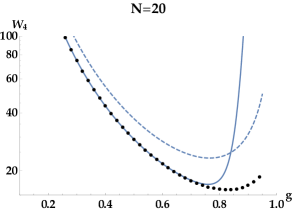
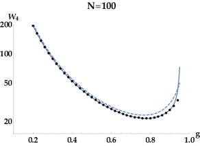
Figure 1: Numerical evaluation of the Wilson loop $\widehat{W}_{4}$ (the hat means that we stripped off the exponential prefactor as explained in the text). Left and right panels are for $N=20,100$. Black dots show the exact high precision numerical evaluation of the exact loop. The solid blue line is the full expansion (4.2), while the dashed line is its lowest leading order at large $N$. The vertical scale is logarithmic to improve data visualization.

4.3 A general formula for the next-to-leading order expansion of general $W_{k}^{\rm inst}$

The fact that (77) starts with $R=1+\dots$ has an important consequence. At the leading instanton level, the only terms in the $k$-th Periwal-Shevitz recursion that play a role are those linear in $f$, i.e. the pair $f_{n+k}+f_{n-k}$, see (3.2), (3.2) and (B). This means that we can work out the procedure illustrated in Sec. (4.2) parametrically in $k$. This is a major simplification given the growing complexity of the recursion with increasing $k$ At leading order in the $g_{s}$ expansion, we obtain

$$R_{0}^{(1),k}(z;\rho)=\frac{1}{\sqrt{z^{2}-1}}\,\bigg{[}1+(-1)^{k}\sinh(k\,\cosh^{-1}(z))\,\rho+\mathcal{O}(\rho^{2})\bigg{]}.$$ (85)

From this expression, a straightforward calculation gives the generalization of the leading term in (4.1,94,4.2) to all $k$. It reads

$$W_{k}^{\rm inst} =\frac{e^{-2\,N\,S(g)}}{4\,\pi\,N^{2}}\,\bigg{[}(-1)^{k}\frac{g}{1-g^{2}}\,\mathscr{U}_{k-1}\left(\frac{1}{g}\right)+\mathcal{O}(N^{-1})\bigg{]},$$ (86)

where $\mathscr{U}_{n}(x)$ are Chebyshev polynomials of the second kind. The compact relation (86) can be checked against (2.1). Indeed, at the leading instanton level we can simply replace

$$w_{1}=\frac{g}{2}+\frac{e^{-2\,N\,S(g)}}{4\,\pi\,N^{2}}\,\frac{g}{g^{2}-1}+\cdots,\quad w_{k\geq 2}=\frac{e^{-2\,N\,S(g)}}{4\,\pi\,N^{2}}\,\widehat{w}_{k}+\cdots,$$ (87)

and we get

$$\sum_{n=2}^{\infty}\widehat{w}_{n}\,x^{n} =\frac{g\,x^{2}\,(2+g\,x)}{(1-g^{2})(g+2x+gx^{2})},$$ (88)

which is indeed equivalent to (86) using the generating function of Chebyshev polynomials. The reason why we can use (2.1) is once again that subleading corrections to large $N$ factorization do not affect the leading term in (86).

Further corrections in $1/N$ to (86) can also be worked out starting the perturbative machinery from the initial seed (85). Remarkably, this may be done for a generic even $k$ and continued to odd $k$. After some tedious manipulation, the general expression for the first two corrections to (86) is in full generality

$$W_{k}^{\rm inst} =(-1)^{k}\,\frac{e^{-2\,N\,S(g)}}{4\,\pi\,N^{2}}\,\bigg{\{}\frac{g}{1-g^{2}}\,\mathscr{U}_{k-1}(g^{-1})$$

$$+\frac{1}{N}\,\frac{g}{12\,(1-g^{2})^{5/2}}\bigg{[}18\,g\,k\,\mathscr{T}_{k}(g^{-1})+[3\,(2k^{2}-3)\,g^{2}-6k^{2}-26]\,\mathscr{U}_{k-1}(g^{-1})\bigg{]}$$

$$+\frac{1}{N^{2}}\frac{g}{288\,(1-g^{2})^{4}}\bigg{[}24\,g\,k\,[(11k^{2}-53)\,g^{2}-11k^{2}-52]\,\mathscr{T}_{k}(g^{-1})+$$

$$+[9\,(4k^{4}-28k^{2}+33)\,g^{4}-12\,(6k^{4}+50k^{2}-207)\,g^{2}+36k^{4}+852k^{2}+964]\,\,\mathscr{U}_{k-1}(g^{-1})\bigg{]}$$

$$+\mathcal{O}(N^{-3})\bigg{\}},$$ (89)

where $\mathscr{T}_{k}(x)$ are Chebyshev polynomials of the first kind. Explicit evaluation for $k=1,2,4$ reproduces the previous results. For $k=3$ we find from (4.3)

$$W_{3}^{\rm inst} =\frac{e^{-2\,N\,S(g)}}{4\,\pi\,N^{2}}\,\bigg{[}\frac{g^{2}-4}{g(1-g^{2})}+\frac{1}{N}\frac{45g^{4}-98g^{2}+104}{12g\left(1-g^{2}\right)^{5/2}}+\frac{1}{N^{2}}\frac{945g^{6}-2592g^{4}+676g^{2}-2704}{288g(g^{2}-1)^{4}}+\dots\bigg{]}.$$ (90)

The $1/N$ correction automatically agrees with the result derived in App. (A) where we fixed the $\rho$ part of the Stokes factor $\mathcal{C}$ by a numerical calculation. Here, it is given automatically from the (trivial) continuation of (4.3) from even $k$ to odd $k$. Once again, the expansion (90) is in full agreement with (2.1) at leading instanton order. Similarly, for $W_{5}$ we obtain from (4.3) the expansion

$$W_{5}^{\rm inst} =\frac{e^{-2\,N\,S(g)}}{4\,\pi\,N^{2}}\,\bigg{[}-\frac{g^{4}-12g^{2}+16}{g^{3}\left(1-g^{2}\right)}+\frac{1}{N}\frac{-141g^{6}+1418g^{4}-2568g^{2}+1376}{12g^{3}\left(1-g^{2}\right)^{5/2}}$$

$$+\frac{1}{N^{2}}\frac{-16497g^{8}+122280g^{6}-269908g^{4}+246384g^{2}-88384}{288g^{3}(g^{2}-1)^{4}}+\dots\bigg{]},$$ (91)

that we checked numerically agains the exact value of $W_{5}$ with the expected numerical accuracy ( the difference goes to zero as $N^{-3}$ for a generic fixed $g$).

5 Conclusions

In this paper, we reconsidered the large $N$ expansion of the Gross-Witten-Wadia matrix model and, in particular, of the winding Wilson loops $W_{k}=\frac{1}{N}\langle\text{tr}U^{k}\rangle$. The motivation of our analysis was to test recent numerical results about these expansions. We have presented various analytical algorithms that are able to accurately compute both the perturbative and instanton corrections in the gapless and gapped phases of the GWW model. All the derived expansions are in full agreement with the Schwinger-Dyson prediction when available.

These tools also apply to the treatment of Wilson loops in small representation where the number of boxes of the associated Young tableau is small compared to $N$. In principle, they may be useful to discuss the more interesting cases of large representations where the number of boxes grows $\sim N$, such those relevant for the study of $k$-strings, see for instance Karczmarek:2010ec , or giant Wilson loops Grignani:2009ua . This seems particularly feasible for the instanton corrections. Indeed, the complexity of the Periwal-Shevitz recursion increases with $k$, but most of its terms simply do not enter such calculation, as we explained in the text. For instance, one of our main results is the accurate expansion (4.3) that is fully parametrical in $k$ and may be the starting point for such investigations. Finally, it could be interesting to study the double scaling limit of the winding Wilson loops starting from their computation in terms of the modified Periwal-Shevitz recursion.

Appendix A A technical aside: Fixing the Stokes constant in instanton corrections to odd winding loops

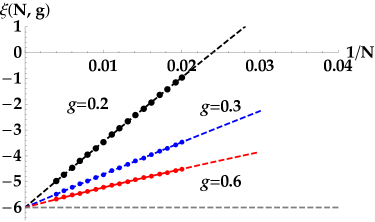
Figure 2: Best estimate $\xi(N,g)$ from the exact $W_{3}(N,g)$ at high precision compared with (94). The three data sets are obtained with $g=0.2\ \text{(black)},0.3\ \text{(blue)},0.6\ \text{(red)}$. Extrapolation to $N\to\infty$ is fully consistent with $\xi=-6$ (horizontal dashed line) independently on $g$.

As we commented in Sec. (4.2) the calculation of instanton corrections to odd winding loops by the Periwal-Shevitz recursion is plagued by a technical problem. Repeating the first steps illustrated in that section in the simplest case of $W_{3}$ we first obtain

$$R^{(1),k=3}_{0}(z;\rho)=\frac{1+(4z^{2}-1)\,\sqrt{z^{2}-1}\,\rho+\mathcal{O}(\rho^{2})}{\sqrt{z^{2}-1}},$$ (92)

and the first correction at small $g_{s}$ expansion reads

$$H^{(1),k=3}_{1}(z)=-3\left(4z^{2}+\frac{1}{2-2z^{2}}-4\right)+\xi,$$ (93)

where $\xi$ is a numerical constant. The associated expansion of $W_{3}^{\rm inst}$ is then obtained from (54) and reads

$$W_{3}^{\rm inst} =\frac{e^{-2\,N\,S(g)}}{4\,\pi\,N^{2}}\,\bigg{[}\frac{g^{2}-4}{g(1-g^{2})}+\frac{1}{N}\,\frac{3g^{4}(4\xi+39)-2g^{2}(6\xi+85)+104}{12g\left(1-g^{2}\right)^{5/2}}+\mathcal{O}(N^{-2})\bigg{]}.$$ (94)

A non zero constant $\xi$ in (93) is not forbidden by parity $z\to-z$ and inspection of (94) does not reveal any obvious way to fix it. This means that further non perturbative information is needed to fix it. A possibility is to compare the exact evaluation of $W_{3}(N,g)$ with the 2-term expansion in (94) and determine the optimal $\xi(N,g)$ that gives equality at the considered $(N,g)$. The correct $\xi$ is obtained as $N\to\infty$ and must be independent on $0<g<1$ as a consistency check. We show this procedure in Fig. (2). We computed the exact $W_{3}(N,g)$ at high precision (400 digits) for $N=50,\dots,250$ at the three values $g=0.2\ \text{(black)},0.3\ \text{(blue)},0.6\ \text{(red)}$. Extrapolation to $N\to\infty$ is fully consistent with $\xi=-6$ with high precision (the relative error is $\sim 10^{-6}$).

As explained in Sec. (4.3), these difficulties and cumbersome procedure can be automatically overcome starting from expressions valid for generic even $k$ and continuing to odd $k$ thus providing a fully analytic result that can be extended to higher $1/N$ accuracy in algorithmic way. Of course, in the specific case of $W_{3}$, the exact result (2.1) is fully reproduced.

Appendix B Periwal-Shevitz recursion relation for $W_{4}$

The $k=4$ case of the recursion (45) is

$$k =4,\quad g_{s}\,(n+1)\,f_{n}=-2(1-f_{n}^{2})\,(f_{n-2}^{3}f_{n-1}^{4}+f_{n}^{3}f_{n-1}^{4}+3f_{n-2}f_{n}^{2}f_{n-1}^{4}+3f_{n-2}^{2}f_{n}f_{n-1}^{4}$$

$$+2f_{n-3}f_{n-2}^{3}f_{n-1}^{3}-2f_{n-3}f_{n-2}f_{n-1}^{3}+2f_{n-3}f_{n-2}^{2}f_{n}f_{n-1}^{3}-2f_{n-3}f_{n}f_{n-1}^{3}+4f_{n}^{3}f_{n+1}f_{n-1}^{3}$$

$$+6f_{n-2}f_{n}^{2}f_{n+1}f_{n-1}^{3}-2f_{n-2}f_{n+1}f_{n-1}^{3}+2f_{n-2}^{2}f_{n}f_{n+1}f_{n-1}^{3}-2f_{n}f_{n+1}f_{n-1}^{3}+f_{n-3}^{2}f_{n-2}^{3}f_{n-1}^{2}$$

$$-f_{n-2}^{3}f_{n-1}^{2}-f_{n-4}f_{n-3}^{2}f_{n-1}^{2}+f_{n-4}f_{n-3}^{2}f_{n-2}^{2}f_{n-1}^{2}-f_{n-4}f_{n-2}^{2}f_{n-1}^{2}-3f_{n-2}f_{n}^{2}f_{n-1}^{2}$$

$$+6f_{n}^{3}f_{n+1}^{2}f_{n-1}^{2}+3f_{n-2}f_{n}^{2}f_{n+1}^{2}f_{n-1}^{2}-f_{n-2}f_{n+1}^{2}f_{n-1}^{2}-4f_{n}f_{n+1}^{2}f_{n-1}^{2}+f_{n-4}f_{n-1}^{2}$$

$$-f_{n-3}^{2}f_{n-2}f_{n-1}^{2}-4f_{n-2}^{2}f_{n}f_{n-1}^{2}+2f_{n-3}f_{n-2}^{2}f_{n}f_{n+1}f_{n-1}^{2}-2f_{n-3}f_{n}f_{n+1}f_{n-1}^{2}-3f_{n}^{2}f_{n+2}f_{n-1}^{2}$$

$$+3f_{n}^{2}f_{n+1}^{2}f_{n+2}f_{n-1}^{2}+2f_{n-2}f_{n}f_{n+1}^{2}f_{n+2}f_{n-1}^{2}-f_{n+1}^{2}f_{n+2}f_{n-1}^{2}-2f_{n-2}f_{n}f_{n+2}f_{n-1}^{2}+f_{n+2}f_{n-1}^{2}$$

$$-2f_{n-3}f_{n-2}^{3}f_{n-1}+4f_{n}^{3}f_{n+1}^{3}f_{n-1}-2f_{n}f_{n+1}^{3}f_{n-1}+2f_{n}f_{n+1}^{3}f_{n+2}^{2}f_{n-1}-2f_{n}f_{n+1}f_{n+2}^{2}f_{n-1}$$

$$+2f_{n-3}f_{n-2}f_{n-1}-2f_{n-3}f_{n-2}^{2}f_{n}f_{n-1}+2f_{n-3}f_{n}f_{n-1}-6f_{n-2}f_{n}^{2}f_{n+1}f_{n-1}+2f_{n-2}f_{n+1}f_{n-1}$$

$$-2f_{n-2}^{2}f_{n}f_{n+1}f_{n-1}+6f_{n}^{2}f_{n+1}^{3}f_{n+2}f_{n-1}-2f_{n+1}^{3}f_{n+2}f_{n-1}-6f_{n}^{2}f_{n+1}f_{n+2}f_{n-1}+2f_{n+1}f_{n+2}f_{n-1}$$

$$-2f_{n}f_{n+1}^{2}f_{n+3}f_{n-1}+2f_{n}f_{n+1}^{2}f_{n+2}^{2}f_{n+3}f_{n-1}-2f_{n}f_{n+2}^{2}f_{n+3}f_{n-1}+2f_{n}f_{n+3}f_{n-1}+f_{n}^{3}f_{n+1}^{4}$$

$$-f_{n-3}^{2}f_{n-2}^{3}+f_{n+1}^{4}f_{n+2}^{3}-f_{n+1}^{2}f_{n+2}^{3}+f_{n-4}f_{n-3}^{2}-f_{n-4}f_{n-3}^{2}f_{n-2}^{2}+f_{n-4}f_{n-2}^{2}-3f_{n-2}f_{n}^{2}f_{n+1}^{2}$$

$$+f_{n-2}f_{n+1}^{2}+3f_{n}f_{n+1}^{4}f_{n+2}^{2}-4f_{n}f_{n+1}^{2}f_{n+2}^{2}+f_{n}f_{n+2}^{2}+f_{n+1}^{2}f_{n+2}^{3}f_{n+3}^{2}-f_{n+2}^{3}f_{n+3}^{2}$$

$$-f_{n+1}^{2}f_{n+2}f_{n+3}^{2}+f_{n+2}f_{n+3}^{2}-f_{n-4}+f_{n-3}^{2}f_{n-2}+f_{n-2}^{2}f_{n}-2f_{n-3}f_{n-2}^{2}f_{n}f_{n+1}+2f_{n-3}f_{n}f_{n+1}$$

$$+3f_{n}^{2}f_{n+1}^{4}f_{n+2}-3f_{n}^{2}f_{n+1}^{2}f_{n+2}-2f_{n-2}f_{n}f_{n+1}^{2}f_{n+2}+2f_{n-2}f_{n}f_{n+2}-2f_{n}f_{n+1}^{3}f_{n+3}+2f_{n+1}^{3}f_{n+2}^{3}f_{n+3}$$

$$-2f_{n+1}f_{n+2}^{3}f_{n+3}+2f_{n}f_{n+1}^{3}f_{n+2}^{2}f_{n+3}-2f_{n}f_{n+1}f_{n+2}^{2}f_{n+3}+2f_{n}f_{n+1}f_{n+3}-2f_{n+1}^{3}f_{n+2}f_{n+3}$$

$$+2f_{n+1}f_{n+2}f_{n+3}+f_{n+1}^{2}f_{n+4}-f_{n+1}^{2}f_{n+2}^{2}f_{n+4}+f_{n+2}^{2}f_{n+4}-f_{n+1}^{2}f_{n+3}^{2}f_{n+4}+f_{n+1}^{2}f_{n+2}^{2}f_{n+3}^{2}f_{n+4}$$

$$-f_{n+2}^{2}f_{n+3}^{2}f_{n+4}+f_{n+3}^{2}f_{n+4}-f_{n+4}).$$ (95)

References

- (1) E. Brézin and S. R. Wadia, The large N expansion in quantum field theory and statistical physics: from spin systems to 2-dimensional gravity. World scientific, 1993.
- (2) P. Rossi, M. Campostrini and E. Vicari, The Large N expansion of unitary matrix models, Phys. Rept. 302 (1998) 143–209, [hep-lat/9609003].
- (3) G. Akemann, J. Baik and P. Di Francesco, The Oxford handbook of random matrix theory. Oxford University Press, 2011.
- (4) C. B. Wang, Application of integrable systems to phase transitions. Springer, 2013.
- (5) H. E. Stanley, Spherical model as the limit of infinite spin dimensionality, Phys. Rev. 176 (1968) 718–722.
- (6) S.-k. Ma, Introduction to the renormalization group, Rev. Mod. Phys. 45 (1973) 589–614.
- (7) G. ’t Hooft, A Planar Diagram Theory for Strong Interactions, Nucl. Phys. B72 (1974) 461.
- (8) D. J. Gross and E. Witten, Possible Third Order Phase Transition in the Large N Lattice Gauge Theory, Phys. Rev. D21 (1980) 446–453.
- (9) J. K. Erickson, G. W. Semenoff and K. Zarembo, Wilson loops in N=4 supersymmetric Yang-Mills theory, Nucl. Phys. B582 (2000) 155–175, [hep-th/0003055].
- (10) N. Drukker and D. J. Gross, An Exact prediction of N=4 SUSYM theory for string theory, J. Math. Phys. 42 (2001) 2896–2914, [hep-th/0010274].
- (11) V. Pestun, Localization of gauge theory on a four-sphere and supersymmetric Wilson loops, Commun. Math. Phys. 313 (2012) 71–129, [0712.2824].
- (12) N. Drukker and B. Fiol, All-genus calculation of Wilson loops using D-branes, JHEP 02 (2005) 010, [hep-th/0501109].
- (13) J. Gomis and F. Passerini, Holographic Wilson Loops, JHEP 08 (2006) 074, [hep-th/0604007].
- (14) J. Gomis and F. Passerini, Wilson Loops as D3-Branes, JHEP 01 (2007) 097, [hep-th/0612022].
- (15) S. A. Hartnoll and S. P. Kumar, Higher rank Wilson loops from a matrix model, JHEP 08 (2006) 026, [hep-th/0605027].
- (16) K. Okuyama and G. W. Semenoff, Wilson loops in N=4 SYM and fermion droplets, JHEP 06 (2006) 057, [hep-th/0604209].
- (17) S. Yamaguchi, Semi-classical open string corrections and symmetric Wilson loops, JHEP 06 (2007) 073, [hep-th/0701052].
- (18) N. Drukker, S. Giombi, R. Ricci and D. Trancanelli, On the D3-brane description of some 1/4 BPS Wilson loops, JHEP 04 (2007) 008, [hep-th/0612168].
- (19) E. I. Buchbinder and A. A. Tseytlin, 1/N correction in the D3-brane description of a circular Wilson loop at strong coupling, Phys. Rev. D89 (2014) 126008, [1404.4952].
- (20) X. Chen-Lin, Symmetric Wilson Loops beyond leading order, SciPost Phys. 1 (2016) 013, [1610.02914].
- (21) M. Marino, Les Houches lectures on matrix models and topological strings, in Les Houches School on Applications of Random Matrices in Physics, 2004. hep-th/0410165.
- (22) S. R. Wadia, A Study of U(N) Lattice Gauge Theory in 2-dimensions (edited version of an unpublished 1979 EFI (U. Chicago) preprint), 1212.2906.
- (23) E. Brezin and J. Zinn-Justin, Renormalization group approach to matrix models, Phys. Lett. B288 (1992) 54–58, [hep-th/9206035].
- (24) S. Higuchi, C. Itoi, S. Nishigaki and N. Sakai, Large N renormalization group approach to matrix models, in Group theoretical methods in physics. Proceedings, 40th Yamada Conference, 20th International Colloquium, Toyonaka, Japan, July 4-9, 1994, 1994. hep-th/9409157.
- (25) V. Periwal and D. Shevitz, Unitary Matrix Models as Exactly Solvable String Theories, Phys. Rev. Lett. 64 (1990) 1326.
- (26) V. Periwal and D. Shevitz, Exactly Solvable Unitary Matrix Models: Multicritical Potentials and Correlations, Nucl. Phys. B344 (1990) 731–746.
- (27) I. R. Klebanov, J. M. Maldacena and N. Seiberg, Unitary and complex matrix models as 1-d type 0 strings, Commun. Math. Phys. 252 (2004) 275–323, [hep-th/0309168].
- (28) H. Liu, Fine structure of Hagedorn transitions, hep-th/0408001.
- (29) L. Alvarez-Gaume, C. Gomez, H. Liu and S. Wadia, Finite temperature effective action, AdS(5) black holes, and 1/N expansion, Phys. Rev. D71 (2005) 124023, [hep-th/0502227].
- (30) E. Witten, Anti-de Sitter space, thermal phase transition, and confinement in gauge theories, Adv. Theor. Math. Phys. 2 (1998) 505–532, [hep-th/9803131].
- (31) M. Marino, Nonperturbative effects and nonperturbative definitions in matrix models and topological strings, JHEP 12 (2008) 114, [0805.3033].
- (32) S. H. Shenker, The strength of nonperturbative effects in string theory, in Random surfaces and quantum gravity, pp. 191–200. Springer, 1991.
- (33) F. David, Phases of the large N matrix model and nonperturbative effects in 2-d gravity, Nucl. Phys. B348 (1991) 507–524.
- (34) P. V. Buividovich, G. V. Dunne and S. N. Valgushev, Complex Path Integrals and Saddles in Two-Dimensional Gauge Theory, Phys. Rev. Lett. 116 (2016) 132001, [1512.09021].
- (35) G. Alvarez, L. Martinez Alonso and E. Medina, Complex saddles in the Gross-Witten-Wadia matrix model, Phys. Rev. D94 (2016) 105010, [1610.09948].
- (36) K. Okuyama, Wilson loops in unitary matrix models at finite , JHEP 07 (2017) 030, [1705.06542].
- (37) J. Ambjorn, L. Chekhov, C. F. Kristjansen and Yu. Makeenko, Matrix model calculations beyond the spherical limit, Nucl. Phys. B404 (1993) 127–172, [hep-th/9302014].
- (38) S. Mizoguchi, On unitary / hermitian duality in matrix models, Nucl. Phys. B716 (2005) 462–486, [hep-th/0411049].
- (39) D. Bessis, A New Method in the Combinatorics of the Topological Expansion, Commun. Math. Phys. 69 (1979) 147.
- (40) D. Bessis, C. Itzykson and J. B. Zuber, Quantum field theory techniques in graphical enumeration, Adv. Appl. Math. 1 (1980) 109–157.
- (41) P. Di Francesco, P. H. Ginsparg and J. Zinn-Justin, 2-D Gravity and random matrices, Phys. Rept. 254 (1995) 1–133, [hep-th/9306153].
- (42) Y. Y. Goldschmidt, 1/ Expansion in Two-dimensional Lattice Gauge Theory, J. Math. Phys. 21 (1980) 1842.
- (43) I. Bars and F. Green, Complete Integration of U () Lattice Gauge Theory in a Large Limit, Phys. Rev. D20 (1979) 3311.
- (44) Yu. M. Makeenko and A. A. Migdal, Exact Equation for the Loop Average in Multicolor QCD, Phys. Lett. 88B (1979) 135.
- (45) A. A. Migdal, Loop Equations and 1/N Expansion, Phys. Rept. 102 (1983) 199–290.
- (46) G. Paffuti and P. Rossi, A Solution of Wilson’s Loop Equation in Lattice QCD in Two-dimensions, Phys. Lett. 92B (1980) 321–323.
- (47) S. R. Wadia, On the Dyson-schwinger Equations Approach to the Large Limit: Model Systems and String Representation of Yang-Mills Theory, Phys. Rev. D24 (1981) 970.
- (48) D. Friedan, Some Nonabelian Toy Models in the Large Limit, Commun. Math. Phys. 78 (1981) 353.
- (49) F. Green and S. Samuel, Chiral Models: Their Implication for Gauge Theories and Large , Nucl. Phys. B190 (1981) 113–150.
- (50) G. Akemann and P. H. Damgaard, Wilson loops in =4 supersymmetric Yang-Mills theory from random matrix theory, Phys. Lett. B513 (2001) 179, [hep-th/0101225].
- (51) M. Marino, R. Schiappa and M. Weiss, Nonperturbative Effects and the Large-Order Behavior of Matrix Models and Topological Strings, Commun. Num. Theor. Phys. 2 (2008) 349–419, [0711.1954].
- (52) Yu. Makeenko, Loop equations in matrix models and in 2-D quantum gravity, Mod. Phys. Lett. A6 (1991) 1901–1913.
- (53) D. J. Gross and A. A. Migdal, Nonperturbative Two-Dimensional Quantum Gravity, Phys. Rev. Lett. 64 (1990) 127.
- (54) D. J. Gross and A. A. Migdal, A Nonperturbative Treatment of Two-dimensional Quantum Gravity, Nucl. Phys. B340 (1990) 333–365.
- (55) J. L. Karczmarek, G. W. Semenoff and S. Yang, Comments on k-Strings at Large N, JHEP 03 (2011) 075, [1012.5875].
- (56) G. Grignani, J. L. Karczmarek and G. W. Semenoff, Hot Giant Loop Holography, Phys. Rev. D82 (2010) 027901, [0904.3750].