Robust stability conditions for feedback interconnections of distributed-parameter negative imaginary systems

Abstract

Sufficient and necessary conditions for the stability of positive feedback interconnections of negative imaginary systems are derived via an integral quadratic constraint (IQC) approach. The IQC framework accommodates distributed-parameter systems with irrational transfer function representations, while generalising existing results in the literature and allowing exploitation of flexibility at zero and infinite frequencies to reduce conservatism in the analysis. The main results manifest the important property that the negative imaginariness of systems gives rise to a certain form of IQCs on positive frequencies that are bounded away from zero and infinity. Two additional sets of IQCs on the DC and instantaneous gains of the systems are shown to be sufficient and necessary for closed-loop stability along a homotopy of systems.

, ,

1 Introduction

The notion of negative imaginary systems was introduced in (Lanzon and Petersen,, 2008; Petersen and Lanzon,, 2010) as a natural counterpart to positive real systems (Anderson and Vongpanitllerd,, 2007; Khalil,, 2002; Bao and Lee,, 2007; van der Schaft,, 2016). The negative imaginary property commonly arises from the dynamics of a lightly damped structure with colocated force actuators and position sensors (such as piezoelectric sensors) (Bhikkaji and Moheimani,, 2009; Petersen and Lanzon,, 2010). Such a system exhibits positive real dynamics from the force input to the velocity output, but negative imaginary dynamics from the force input to the position output, whose transfer function may be of relative degree 2. Furthermore, negative imaginary systems theory may also be employed to study certain systems that are not passive, for which positive real results do not hold. Another area where negative imaginary dynamics can be found is that of nano-positioning systems (Devasia et al.,, 2007). Owing to the prevalence of negative imaginary properties in real world applications, such systems have been studied extensively in the literature (Lanzon and Petersen,, 2008; Petersen and Lanzon,, 2010; Xiong et al.,, 2010; Das et al.,, 2013). Feedback interconnections of negative imaginary systems are interpreted from a geometric Hamiltonian systems viewpoint in (van der Schaft,, 2011). In (Wang et al.,, 2015), the problem of robust output consensus of networked negative imaginary systems is considered. Characterisations of negative imaginary systems with symmetric irrational transfer functions are considered in (Ferrante and Ntogramatzidis,, 2013; Ferrante et al.,, 2015). A nonlinear generalisation of negative imaginary dynamics, termed counterclockwise input-output dynamics, is given in (Angeli,, 2006).

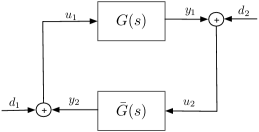
Figure 1: Positive feedback interconnection of negative imaginary systems.

The robustness of feedback interconnections of open-loop stable negative imaginary systems is investigated in (Lanzon and Petersen,, 2008) as a parallel to the positive real stability results (Anderson and Vongpanitllerd,, 2007); see Figure 1. It is shown that if the instantaneous gain of $\bar{G}$ is positive semidefinite, i.e. $\bar{G}(\infty)\geq 0$, and the product of the instantaneous gains of $\bar{G}$ and $G$ is 0, i.e. $G(\infty)\bar{G}(\infty)=0$, then the closed-loop system $[G,\bar{G}]$ is internally stable if, and only if, the DC gain condition $\bar{\lambda}(G(0)\bar{G}(0))<1$ is satisfied, where $\bar{\lambda}$ denotes the spectral radius. This result is further generalised in (Xiong et al.,, 2010) to the case where $G$ may have imaginary-axis poles that are not located at the origin. Physical interpretations of these results in terms of mass-spring-damper systems and RLC electrical networks are provided in (Petersen,, 2015). In particular, it is demonstrated using the negative imaginary theory that certain mass-spring-damper systems with negative spring constants or RLC networks with negative inductances or capacitances are stable, whereas the standard positive real theory is inapplicable to such non-passive systems. These stability conditions are robust in the sense that they are invariant to negative-imaginary perturbations on the systems, provided that the aforementioned gain conditions are not violated. Stability conditions for negative imaginary systems with poles at the origin are studied in (Mabrok et al.,, 2014).

When the presuppositions of the stability theorems in (Lanzon and Petersen,, 2008; Xiong et al.,, 2010) do not hold, such as $\bar{G}(\infty)$ being sign-indefinite or $G(\infty)\bar{G}(\infty)\neq 0$, the DC gain condition $\bar{\lambda}(G(0)\bar{G}(0))<1$ is not necessary. This paper derives generic sufficient and necessary conditions for feedback stability of negative imaginary systems with respect to a specified homotopy using the theory of integral quadratic constraints (IQC) (Megretski and Rantzer,, 1997; Megretski et al.,, 2010; Cantoni et al.,, 2013). In particular, it is established that the negative imaginary properties of the systems give rise to complementary IQCs on a set of frequencies which do not include 0 and $\infty$ but can be arbitrarily large. This interpretation clarifies the role of negative imaginariness in robust feedback stability analysis. Furthermore, it leads to the observation that feedback stability follows if, and only if, there exist constant multipliers such that the corresponding complementary IQCs hold at frequencies of $0$ and $\infty$, of which the condition in (Lanzon and Petersen,, 2008) that $\bar{\lambda}(G(0)\bar{G}(0))<1$, $\bar{G}(\infty)\geq 0$, and $G(\infty)\bar{G}(\infty)=0$ is a special case. The robust stability result is shown to extend to negative imaginary systems that are only marginally stable, i.e. have poles on the imaginary axis. To this end, a recently developed notion of IQCs for marginally stable systems from (Khong et al.,, 2016) is employed to conclude closed-loop stability. This paper considers distributed-parameter linear time-invariant systems that admit irrational transfer functions. Such a class of systems corresponds to infinite-dimensional state-space systems in the time domain (Curtain and Zwart,, 1995). Furthermore, no explicit state-space realisations are exploited in any of the proofs for the main results. This contrasts the preceding works (Lanzon and Petersen,, 2008; Xiong et al.,, 2010), where state matrices and the negative imaginary lemma (the counterpart to the positive real lemma) are heavily employed. Preliminary results in this direction can be found in (Khong et al.,, 2015), where only sufficient IQC conditions were given for the class of proper real-rational transfer functions. Moreover, the results have been further strengthened in this paper via the removal of an assumption on a certain residual matrix and a reconciliation with the existing results is provided. It is noteworthy that similar necessary and sufficient IQC based results for robustness analysis involving time-delays can be found in (Scorletti,, 1997) and the idea of combining IQCs which hold on subsets of the imaginary axis can be located in (Jun and Safonov,, 2002).

The paper evolves along the following lines. The next section introduces the notation of the paper and defines the classes of negative imaginary systems considered. Robust stability of feedback interconnections of stable negative imaginary systems is examined in Section 3. Sufficient robust stability conditions for negative imaginary systems with imaginary-axis poles are derived in Section 4. The necessity of IQC conditions for feedback stability of negative imaginary systems is established in Section 5, and a reconciliation with the existing robustness results takes place in Section 6. Two numerical examples are given in Section 7 to illustrate the theory. Finally, concluding remarks are provided in Section 8.

2 Notation and preliminaries

The notation used in this paper is defined in this section. Let $\mathbb{R}$ and $\mathbb{C}$ denote, respectively, the real and complex numbers. The real part of an $s\in\mathbb{C}$ is denoted as $\Re(s)$. $\mathbb{C}_{+}$ denotes the open right half plane and $\bar{\mathbb{C}}_{+}$ its closure. Given an $A\in\mathbb{C}^{m\times n}$ (resp. $\mathbb{R}^{m\times n}$), $A^{*}\in\mathbb{C}^{n\times m}$ (resp. $A^{T}\in\mathbb{R}^{n\times m}$) denotes its complex conjugate transpose (resp. transpose). Denote by $\bar{\sigma}(A)$ and $\underline{\sigma}(A)$, the largest and smallest singular values of matrix $A$, respectively, and by $\bar{\lambda}(B)$, the spectral radius of $B$. $I_{n}$ denotes the identity matrix of dimensions $n\times n$. Subsequently, the subscript $n$ will often be dropped for simplicity.

Let $\boldsymbol{\mathcal{R}}^{n\times m}$ denote the set of real-rational proper transfer function matrices of dimensions $n\times m$ and

$$\boldsymbol{\rm H}_{\infty}^{n\times m}\!:=\!\left\{X:\mathbb{C}\to\mathbb{C}^{n\times m}\text{ (a.e.)}\left|\begin{array}[]{l}X\text{ is analytic in }\mathbb{C}_{+}\\ \displaystyle\sup_{s\in\mathbb{C}_{+}}\bar{\sigma}(X(s))<\infty\end{array}\right.\!\!\right\}$$

the set of stable transfer functions. The norm of the elements in $\boldsymbol{\rm H}_{\infty}$ is denoted $\|\cdot\|_{\infty}$. Let $\boldsymbol{\mathrm{C}}$ be the class of functions $f:\mathbb{C}\to\mathbb{C}^{n\times m}$ (a.e.) that are continuous on $j\mathbb{R}\cup\{\infty\}$, and $\boldsymbol{\mathrm{S}}:=\boldsymbol{\rm H}_{\infty}\cap\boldsymbol{\mathrm{C}}$. The positive feedback interconnection of two transfer functions $G$ and $\bar{G}$, denoted by $[G,\bar{G}]$, is described by:

$$\begin{bmatrix}{d_{1}}\\ {d_{2}}\end{bmatrix}=\begin{bmatrix}{I}&{-\bar{G}}\\ {-G}&{I}\end{bmatrix}\begin{bmatrix}{u_{1}}\\ {u_{2}}\end{bmatrix};$$

see Figure 1.

Definition 1.

A positive feedback interconnection of $G$ and $\bar{G}$ is said to be internally stable if

$$\begin{bmatrix}{I}&{-\bar{G}}\\ {-G}&{I}\end{bmatrix}^{-1}=\begin{bmatrix}{I+\bar{G}(I-G\bar{G})^{-1}G}&{\bar{G}(I-G\bar{G})^{-1}}\\ {(I-G\bar{G})^{-1}G}&{(I-G\bar{G})^{-1}}\end{bmatrix}$$

is an element in $\boldsymbol{\rm H}_{\infty}$.

Define

$$\hat{\boldsymbol{\mathrm{N}}} :=\{R\in\boldsymbol{\mathrm{S}}^{n\times n}:$$

$$\qquad j[R(j\omega)-R(j\omega)^{*}]\geq 0\;\forall\omega\in(0,\infty)\}\quad\text{and}$$

$$\boldsymbol{\mathrm{N}}_{s} :=\{R\in\boldsymbol{\mathrm{S}}^{n\times n}:$$

$$\qquad j[R(j\omega)-R(j\omega)^{*}]>0\;\forall\omega\in(0,\infty)\}\subset\hat{\boldsymbol{\mathrm{N}}}.$$

$\hat{\boldsymbol{\mathrm{N}}}$ denotes the set of stable negative imaginary transfer functions, while $\boldsymbol{\mathrm{N}}_{s}$ denotes the set of strictly negative imaginary transfer functions. The set of stable (strictly) negative imaginary real-rational proper transfer functions defined in (Lanzon and Petersen,, 2008) is a subclass of $\hat{\boldsymbol{\mathrm{N}}}$ ($\boldsymbol{\mathrm{N}}_{s}$). In particular, an $R\in\boldsymbol{\mathcal{R}}\cap\hat{\boldsymbol{\mathrm{N}}}$ satisfies $R(0)=R(0)^{T}\in\mathbb{R}^{n\times n}$ and $R(\infty)=R(\infty)^{T}\in\mathbb{R}^{n\times n}$ (Lanzon and Petersen,, 2008, Lem. 2). Therefore, it follows that $j[R(j\omega)-R(j\omega)^{*}]=0$ when $\omega=0$ or $\omega=\infty$. The set of negative imaginary transfer functions is defined below.

Definition 2.

A transfer function $R:\mathbb{C}\to\mathbb{C}^{n\times n}$ (a.e.) is said to be negative imaginary if

1. $R$ is analytic in $\Re(s)>0$ and has no singularities at $s=0$ and $s=\infty$;

2. $R(\cdot+\epsilon)\in\boldsymbol{\rm H}_{\infty}$ for some $\epsilon>0$;

3. $R$ has at most a finite number of singularities on the imaginary axis and they appear as complex conjugate pairs;

4. $R(j\omega)$ is continuous on $j\mathbb{R}$ except when $j\omega$ is a singularity;

5. $j[R(j\omega)-R(j\omega)^{*}]\geq 0$ for all $\omega\in(0,\infty)$ except values $\omega$ where $j\omega$ is a singularity of $R(s)$;

6. if $s=j\omega_{0}$ with $\omega_{0}\in(0,\infty)$ is a singularity of $R(s)$, then it is a simple pole and the residue matrix $\displaystyle\lim_{s\rightarrow j\omega_{0}}(s-j\omega_{0})jR(s)$ is Hermitian and positive semidefinite.

Denote by $\boldsymbol{\mathrm{N}}$ the set of negative imaginary transfer functions. Notice that $\boldsymbol{\mathrm{N}}_{s}\subset\hat{\boldsymbol{\mathrm{N}}}\subset\boldsymbol{\mathrm{N}}$. The set of negative imaginary real-rational proper transfer functions defined in (Xiong et al.,, 2010) is a subclass of $\boldsymbol{\mathrm{N}}$. It is noted here that the definitions given above differ from those in (Ferrante and Ntogramatzidis,, 2013; Ferrante et al.,, 2015) in that no efforts have been made here to link the definitions to the classical positive real theory. Instead, only the properties crucial to the robust stability conditions to be derived in the next sections are stipulated.

In order to accommodate possibly irrational transfer functions with poles on the imaginary axis in this paper, some background material on IQCs needs to be stated. To this end, the following notational definitions are important. Given an $\epsilon>0$ and a point $jq\in j\mathbb{R}$, define the semi-circle of radius $\epsilon$ in the right-half plane as

$$\SS_{\epsilon}(jq):=\{s\in\mathbb{C}:|s-jq|=\epsilon,\Re(s)>0\}$$

and $\SS_{0}(jq):=\{\}$. Given a finite ordered set $j\mathcal{Q}=\{jq_{1},jq_{2},\ldots,jq_{K}\}\subset j\mathbb{R}$ with $q_{1}>q_{2}>\ldots>q_{K}$, define a contour parameterised by $\epsilon\geq 0$ as

$$\begin{split}\mathcal{C}_{\epsilon}(j\mathcal{Q}):=j[q_{1}+\epsilon,\infty)&\cup\SS_{\epsilon}(jq_{1})\cup j[q_{2}+\epsilon,q_{1}-\epsilon]\\ &\cup\SS_{\epsilon}(jq_{2})\cup j[q_{3}+\epsilon,q_{2}-\epsilon]\\ &\qquad\qquad\vdots\\ &\cup\SS_{\epsilon}(jq_{K})\cup j(-\infty,q_{K}-\epsilon].\end{split}$$ (1)

that is, a straight line on the imaginary axis indented to the right of every point in $j\mathcal{Q}$ by a semi-circle of radius $\epsilon$. In particular, notice that $C_{0}(j\mathcal{Q})=j\mathbb{R}$ for any $j\mathcal{Q}\subset j\mathbb{R}$. Denote by $\mathcal{C}_{\epsilon}^{+}(j\mathcal{Q})$ the open half plane that lies to the right of $\mathcal{C}_{\epsilon}(j\mathcal{Q})$ defined in (1), i.e.

$$\mathcal{C}_{\epsilon}^{+}(j\mathcal{Q}):=\{s=\sigma+j\omega\in\mathbb{C}\ |\ \bar{\sigma}+j\omega\in\mathcal{C}_{\epsilon}(j\mathcal{Q})\Rightarrow\sigma>\bar{\sigma}\},$$

and $\bar{\mathcal{C}}_{\epsilon}^{+}(j\mathcal{Q})$ its closure. Let $\boldsymbol{\mathrm{C}}_{\epsilon}(j\mathcal{Q})$ be the class of functions continuous on $\mathcal{C}_{\epsilon}(j\mathcal{Q})\cup\{\infty\}$. Given $X\in\boldsymbol{\mathrm{C}}_{\epsilon}(j\mathcal{Q})^{n\times m}$, define $\|X\|_{\boldsymbol{\mathrm{C}}_{\epsilon}(j\mathcal{Q})}:=\sup_{s\in\mathcal{C}_{\epsilon}(j\mathcal{Q})}\bar{\sigma}(X(s))$. Let $\boldsymbol{\mathrm{S}}_{\epsilon}(j\mathcal{Q})$ be the subclass of $\boldsymbol{\mathrm{C}}_{\epsilon}(j\mathcal{Q})$ containing functions that have analytic continuation into $\mathcal{C}_{\epsilon}^{+}(j\mathcal{Q})$. Note that $\boldsymbol{\mathrm{S}}=\boldsymbol{\mathrm{S}}_{0}(j\mathcal{Q})\subset\boldsymbol{\mathrm{S}}_{\epsilon}(j\mathcal{Q})$ for all $\epsilon\geq 0$.

The following result can be established using the arguments in (Khong et al.,, 2016, Thm. 4.4 and 4.5). It has further been generalised in (Khong et al.,, 2017).

Proposition 3.

Given $G\in\boldsymbol{\mathrm{S}}_{\epsilon}(j\mathcal{Q})$ and $\bar{G}\in\boldsymbol{\mathrm{S}}_{\epsilon}(j\mathcal{Q})$, the closed-loop transfer function of the feedback interconnection $[G,\bar{G}]$

$$H:=\begin{bmatrix}{I}&{-\bar{G}}\\ {-G}&{I}\end{bmatrix}^{-1}\in\boldsymbol{\mathrm{S}}_{\epsilon}(j\mathcal{Q})$$

for all $\epsilon>0$, if there exist a bounded $\Pi\in\boldsymbol{\mathrm{C}}^{(n+m)\times(n+m)}$ and $\eta>0$ such that $\Pi(j\omega)=\Pi(j\omega)^{*}$ for all $\omega\in\mathbb{R}$ and the following complementary IQC conditions hold:

1. for all $\omega\in\mathbb{R}\setminus\mathcal{Q}$,

   $$\begin{bmatrix}{\bar{G}(j\omega)}\\ {I}\end{bmatrix}^{*}\Pi(j\omega)\begin{bmatrix}{\bar{G}(j\omega)}\\ {I}\end{bmatrix}\leq-\eta I;$$

2. for all $\omega\in\mathbb{R}\setminus\mathcal{Q},\tau\in[0,1]$,

   $$\begin{bmatrix}{I}\\ {\tau G(j\omega)}\end{bmatrix}^{*}\Pi(j\omega)\begin{bmatrix}{I}\\ {\tau G(j\omega)}\end{bmatrix}\geq 0.$$

Furthermore, when $j\mathcal{Q}=\{\}$, $\epsilon$ can be taken to be $0$, whereby $\boldsymbol{\mathrm{S}}_{0}(\{\})=\boldsymbol{\mathrm{S}}\subset\boldsymbol{\rm H}_{\infty}$.

3 Stable negative imaginary transfer functions

In this section, sufficient IQC conditions which guarantee closed-loop stability with stable negative imaginary systems are derived. The proof methods in this section will be reused in the subsequent section where systems with nonzero imaginary-axis poles are accommodated. They involve constructing a 3-part IQC, each of which is valid for a different frequency range. An intuitive depiction of the theorem below is provided after the proof.

Theorem 4.

Given $G\in\hat{\boldsymbol{\mathrm{N}}}^{n\times n}$ and $\bar{G}\in\boldsymbol{\mathrm{N}}_{s}^{n\times n}$, suppose there exist $\Pi_{0}=\Pi_{0}^{*}\in\mathbb{C}^{2n\times 2n}$, $\Pi_{\infty}=\Pi_{\infty}^{*}\in\mathbb{C}^{2n\times 2n}$ such that for some $\bar{\epsilon}>0$ and all $\tau\in[0,1]$,

$$\begin{split}\begin{bmatrix}{\bar{G}(0)}\\ {I}\end{bmatrix}^{*}\Pi_{0}\begin{bmatrix}{\bar{G}(0)}\\ {I}\end{bmatrix}&\leq-\bar{\epsilon}I;\\ \begin{bmatrix}{I}\\ {\tau G(0)}\end{bmatrix}^{*}\Pi_{0}\begin{bmatrix}{I}\\ {\tau G(0)}\end{bmatrix}&\geq 0\end{split}$$ (2)

and

$$\begin{split}\begin{bmatrix}{\bar{G}(\infty)}\\ {I}\end{bmatrix}^{*}\Pi_{\infty}\begin{bmatrix}{\bar{G}(\infty)}\\ {I}\end{bmatrix}&\leq-\bar{\epsilon}I;\\ \begin{bmatrix}{I}\\ {\tau G(\infty)}\end{bmatrix}^{*}\Pi_{\infty}\begin{bmatrix}{I}\\ {\tau G(\infty)}\end{bmatrix}&\geq 0.\end{split}$$ (3)

Then the feedback interconnection $[\tau G,\bar{G}]$ is internally stable for all $\tau\in[0,1]$.

Let $\hat{\Pi}_{0}:=2\Pi_{0}+\mu I$ and $\hat{\Pi}_{\infty}:=2\Pi_{\infty}+\mu I$. Then for sufficiently small $\mu>0$, the inequalities (2) and (3) imply, respectively,

$$\begin{bmatrix}{\bar{G}(0)}\\ {I}\end{bmatrix}^{*}\hat{\Pi}_{0}\begin{bmatrix}{\bar{G}(0)}\\ {I}\end{bmatrix} \leq-\epsilon I;$$

$$\begin{bmatrix}{I}\\ {\tau G(0)}\end{bmatrix}^{*}\hat{\Pi}_{0}\begin{bmatrix}{I}\\ {\tau G(0)}\end{bmatrix} \geq\epsilon I$$

and

$$\begin{bmatrix}{\bar{G}(\infty)}\\ {I}\end{bmatrix}^{*}\hat{\Pi}_{\infty}\begin{bmatrix}{\bar{G}(\infty)}\\ {I}\end{bmatrix} \leq-\epsilon I;$$

$$\begin{bmatrix}{I}\\ {\tau G(\infty)}\end{bmatrix}^{*}\hat{\Pi}_{\infty}\begin{bmatrix}{I}\\ {\tau G(\infty)}\end{bmatrix} \geq\epsilon I$$

for some $\epsilon>0$ and all $\tau\in[0,1]$. By the continuity of $G\in\boldsymbol{\mathrm{S}}$ and $\bar{G}\in\boldsymbol{\mathrm{S}}$ on $j\mathbb{R}$, these imply there exist sufficiently small $\underline{\Omega}>0$ and sufficiently large $\bar{\Omega}>0$ such that

$$\begin{split}\begin{bmatrix}{\bar{G}(j\omega)}\\ {I}\end{bmatrix}^{*}\hat{\Pi}_{0}\begin{bmatrix}{\bar{G}(j\omega)}\\ {I}\end{bmatrix}&\leq-\frac{\epsilon}{2}I;\\ \begin{bmatrix}{I}\\ {\tau G(j\omega)}\end{bmatrix}^{*}\hat{\Pi}_{0}\begin{bmatrix}{I}\\ {\tau G(j\omega)}\end{bmatrix}&\geq\frac{\epsilon}{2}I\end{split}$$ (4)

for all $\omega\in[0,\underline{\Omega}]$, $\tau\in[0,1]$ and

$$\begin{split}\begin{bmatrix}{\bar{G}(j\omega)}\\ {I}\end{bmatrix}^{*}\hat{\Pi}_{\infty}\begin{bmatrix}{\bar{G}(j\omega)}\\ {I}\end{bmatrix}&\leq-\frac{\epsilon}{2}I\\ \begin{bmatrix}{I}\\ {\tau G(j\omega)}\end{bmatrix}^{*}\hat{\Pi}_{\infty}\begin{bmatrix}{I}\\ {\tau G(j\omega)}\end{bmatrix}&\geq\frac{\epsilon}{2}I\end{split}$$ (5)

for all $\omega\in[\bar{\Omega},\infty]$, $\tau\in[0,1]$. Now note from the definitions of $\hat{\boldsymbol{\mathrm{N}}}$ and $\boldsymbol{\mathrm{N}}_{s}$ that $G\in\hat{\boldsymbol{\mathrm{N}}}$ and $\bar{G}\in\boldsymbol{\mathrm{N}}_{s}$ implies that

$$\begin{split}\begin{bmatrix}{\bar{G}(j\omega)}\\ {I}\end{bmatrix}^{*}\Pi_{m}\begin{bmatrix}{\bar{G}(j\omega)}\\ {I}\end{bmatrix}&\leq 0;\\ \begin{bmatrix}{I}\\ {\tau G(j\omega)}\end{bmatrix}^{*}\Pi_{m}\begin{bmatrix}{I}\\ {\tau G(j\omega)}\end{bmatrix}&\geq 0\end{split}$$ (6)

for all $\tau\in[0,1]$ and $\omega\in[0,\infty)$, where

$$\Pi_{m}:=\begin{bmatrix}{0}&{jI}\\ {-jI}&{0}\end{bmatrix}.$$

Furthermore, there exists $\bar{\eta}>0$ such that

$$\begin{split}\begin{bmatrix}{\bar{G}(j\omega)}\\ {I}\end{bmatrix}^{*}\Pi_{m}\begin{bmatrix}{\bar{G}(j\omega)}\\ {I}\end{bmatrix}&\leq-\bar{\eta}I;\\ \begin{bmatrix}{I}\\ {\tau G(j\omega)}\end{bmatrix}^{*}\Pi_{m}\begin{bmatrix}{I}\\ {\tau G(j\omega)}\end{bmatrix}&\geq 0\end{split}$$ (7)

for all $\tau\in[0,1]$ and $\omega\in[\underline{\Omega},\bar{\Omega}]$. Let $\hat{\Pi}_{m}:=2\Pi_{m}+\bar{\mu}I$, then for sufficiently small $\bar{\mu}>0$, (7) implies that

$$\begin{split}\begin{bmatrix}{\bar{G}(j\omega)}\\ {I}\end{bmatrix}^{*}\hat{\Pi}_{m}\begin{bmatrix}{\bar{G}(j\omega)}\\ {I}\end{bmatrix}&\leq-\eta I;\\ \begin{bmatrix}{I}\\ {\tau G(j\omega)}\end{bmatrix}^{*}\hat{\Pi}_{m}\begin{bmatrix}{I}\\ {\tau G(j\omega)}\end{bmatrix}&\geq\eta I\end{split}$$ (8)

for some $\eta>0$, all $\tau\in[0,1]$ and $\omega\in[\underline{\Omega},\bar{\Omega}]$. Define

$$\gamma_{0}(j\omega):=\left\{\begin{array}[]{ll}1&\quad\omega\in[-\underline{\Omega},\underline{\Omega}]\\ 0&\quad\text{otherwise},\end{array}\right.$$

$$\gamma_{\infty}(j\omega):=\left\{\begin{array}[]{ll}1&\quad\omega\in[\bar{\Omega},\infty)\cup(-\infty,-\bar{\Omega}]\\ 0&\quad\text{otherwise},\end{array}\right.$$

and

$$\Pi(j\omega):=\gamma_{0}(j\omega)\hat{\Pi}_{0}+\hat{\Pi}_{m}+\gamma_{\infty}(j\omega)\hat{\Pi}_{\infty},\omega\in\mathbb{R}.$$ (9)

Combining (4), (5), (6), and (8) yields that

$$\begin{split}\begin{bmatrix}{\bar{G}(j\omega)}\\ {I}\end{bmatrix}^{*}\Pi(j\omega)\begin{bmatrix}{\bar{G}(j\omega)}\\ {I}\end{bmatrix}&\leq-\zeta I;\\ \begin{bmatrix}{I}\\ {\tau G(j\omega)}\end{bmatrix}^{*}\Pi(j\omega)\begin{bmatrix}{I}\\ {\tau G(j\omega)}\end{bmatrix}&\geq 0\end{split}$$ (10)

for all $\omega\in[0,\infty)$, $\tau\in[0,1]$ and some $\zeta>0$. By taking the complex conjugate on both sides of the inequalities, observe that (10) holds for all $\omega\in\mathbb{R}$. The stability of $[\tau G,\bar{G}]$ for $\tau\in[0,1]$ then follows from as a special case of the IQC result in Proposition 3 with $j\mathcal{Q}=\{\}$ and $\epsilon=0$. ∎

The stability conditions in Theorem 4 are robust in the sense that if $[G,\bar{G}]$ is stable, then the feedback interconnection remains stable with respect to negative imaginary perturbations on $G$ and $\bar{G}$ that do not violate the DC and instantaneous gain conditions (2) and (3).

Remark 5.

The proof of Theorem 4 relies on the homotopy approach and the fact that $[\tau G,\bar{G}]$ is stable when $\tau=0$. In particular, perturbation arguments can be used to show that $[\tau G,\bar{G}]$ is stable as one increases $\tau$ from $0$ to $1$. In the case where $\|G^{-1}\|_{\infty}^{-1}$ and $\|\bar{G}^{-1}\|_{\infty}^{-1}$ are both finite, it follows from the large-gain theorem in Zahedzadeh et al., (2008) that $[\tau G,\bar{G}]$ is stable for sufficiently large $\tau$. This allows the use of an alternative homotopy, whereby Theorem 4 can be modified with $\tau\in[0,1]$ replaced by $\tau\geq 1$.

Remark 6.

Note from its proof that the conclusion in Theorem 4 remains valid with (2) and (3) modified into the following forms:

$$\begin{split}\begin{bmatrix}{\tau\bar{G}(0)}\\ {I}\end{bmatrix}^{*}\Pi_{0}\begin{bmatrix}{\tau\bar{G}(0)}\\ {I}\end{bmatrix}&\geq\epsilon I;\\ \begin{bmatrix}{I}\\ {G(0)}\end{bmatrix}^{*}\Pi_{0}\begin{bmatrix}{I}\\ {G(0)}\end{bmatrix}&\leq 0\end{split}$$ (11)

and

$$\begin{split}\begin{bmatrix}{\tau\bar{G}(\infty)}\\ {I}\end{bmatrix}^{*}\Pi_{\infty}\begin{bmatrix}{\tau\bar{G}(\infty)}\\ {I}\end{bmatrix}&\geq\epsilon I;\\ \begin{bmatrix}{I}\\ {G(\infty)}\end{bmatrix}^{*}\Pi_{\infty}\begin{bmatrix}{I}\\ {G(\infty)}\end{bmatrix}&\leq 0.\end{split}$$ (12)

Theorem 4 is established by fabricating a 3-part multiplier $\Pi$ in (9) in such a way that the standard IQC result can be applied to conclude closed-loop stability. In particular, the fact that $G\in\hat{\boldsymbol{\mathrm{N}}}$ and $\bar{G}\in\boldsymbol{\mathrm{N}}_{s}$ implies the complementary IQC inequalities hold for positive frequencies that are bounded from zero and infinity; see (8). The additional matrix inequalities (2) and (3) in the theorem imply the complementary IQC inequalities for sufficiently small and sufficiently large frequencies, i.e. (4) and (5) respectively.

Corollary 7.

Given $G\in\hat{\boldsymbol{\mathrm{N}}}$ and $\bar{G}\in\boldsymbol{\mathrm{N}}_{s}$, suppose $\bar{\sigma}(G(0)\bar{G}(0))<1$ and $\bar{\sigma}(G(\infty)\bar{G}(\infty))<1$, then the feedback interconnection $[\tau G,\bar{G}]$ is internally stable for all $\tau\in[0,1]$.

Note that the hypothesis is equivalent to $\bar{\lambda}(\bar{G}(j\omega)^{*}G(j\omega)^{*}G(j\omega)\bar{G}(j\omega))<1$ for $\omega=0$ and $\omega=\infty$. It follows that the matrix inequalities (2) and (3) in Theorem 4 hold with respect to

$$\Pi_{0}:=\begin{bmatrix}{G(0)^{*}G(0)}&{0}\\ {0}&{-I}\end{bmatrix}$$

and

$$\Pi_{\infty}:=\begin{bmatrix}{G(\infty)^{*}G(\infty)}&{0}\\ {0}&{-I}\end{bmatrix},$$

as required. ∎

4 Negative imaginary transfer functions with imaginary-axis poles

IQC-based conditions for feedback stability of negative imaginary systems with imaginary-axis poles are established in this section. The proofs rely on the arguments detailed in Section 3. In order to accommodate negative imaginary transfer functions with imaginary-axis poles, the generalised version of the IQC result, i.e. Proposition 3, is needed.

Theorem 8.

Given $\bar{G}\in\boldsymbol{\mathrm{N}}_{s}$ and $G\in\boldsymbol{\mathrm{N}}$, suppose there exist $\Pi_{0}$ and $\Pi_{\infty}$ such that for all $\tau\in[0,1]$,

$$\begin{split}\begin{bmatrix}{\bar{G}(0)}\\ {I}\end{bmatrix}^{*}\Pi_{0}\begin{bmatrix}{\bar{G}(0)}\\ {I}\end{bmatrix}&<0;\\ \begin{bmatrix}{I}\\ {\tau G(0)}\end{bmatrix}^{*}\Pi_{0}\begin{bmatrix}{I}\\ {\tau G(0)}\end{bmatrix}&\geq 0,\end{split}$$ (13)

$$\begin{split}\begin{bmatrix}{\bar{G}(\infty)}\\ {I}\end{bmatrix}^{*}\Pi_{\infty}\begin{bmatrix}{\bar{G}(\infty)}\\ {I}\end{bmatrix}&<0;\\ \begin{bmatrix}{I}\\ {\tau G(\infty)}\end{bmatrix}^{*}\Pi_{\infty}\begin{bmatrix}{I}\\ {\tau G(\infty)}\end{bmatrix}&\geq 0,\end{split}$$ (14)

then the feedback interconnection $[\tau G,\bar{G}]$ is internally stable for all $\tau\in[0,1]$.

The same arguments in the proof for Theorem 4 can be used to establish (10) for all $\tau\in[0,1]$ and $\omega\in[0,\infty]\setminus\mathcal{Q}$, where $j\mathcal{Q}$ denotes the set of imaginary-axis poles of $G$. The only additional requirement is that $\underline{\Omega}$ needs to be sufficiently small and $\bar{\Omega}$ sufficiently large so that $\mathcal{Q}\cap[0,\underline{\Omega}]=\{\}$ and $\mathcal{Q}\cap[\bar{\Omega},\infty]=\{\}$. By Proposition 3, this then implies that the closed-loop transfer function

$$H_{\tau}:=\begin{bmatrix}{I}&{-\bar{G}}\\ {-\tau G}&{I}\end{bmatrix}^{-1}\in\boldsymbol{\mathrm{S}}_{\epsilon}(j\mathcal{Q})$$ (15)

for all $\tau\in[0,1]$ and $\epsilon>0$. In what follows, we show that $H_{\tau}$ has also no poles in $j\mathcal{Q}$, which then implies $H_{\tau}\in\boldsymbol{\mathrm{S}}\subset\boldsymbol{\rm H}_{\infty}$, i.e. the feedback interconnection $[\tau G,\bar{G}]$ is stable, for all $\tau\in[0,1]$.

First note that $\bar{G}\in\boldsymbol{\mathrm{N}}_{s}$ implies $\det(\bar{G}(j\omega))\neq 0$ for $\omega\neq 0$. To see this, observe that if $\det(\bar{G}(j\omega_{0}))=0$ for some $\omega_{0}>0$, then there exists $v\in\mathbb{C}^{n}$ such that $\bar{G}(j\omega_{0})v=0$. It follows that $v^{*}j[\bar{G}(j\omega_{0})-\bar{G}(j\omega_{0})^{*}]v=0$, which violates the supposition that $\bar{G}\in\boldsymbol{\mathrm{N}}_{s}$. As such,

$$\det(\bar{G}(j\omega))\neq 0\quad\forall\omega\in(0,\infty).$$ (16)

This implies that there is no closed right-half plane pole-zero cancellation in the product $\tau G(s)\bar{G}(s)$, since $\tau G\in\boldsymbol{\mathrm{N}}$ has no poles at the origin. Therefore, for any $\omega_{0}\in\mathbb{R}$, $j\omega_{0}$ is a pole of $H_{\tau}(s)$ if, and only if, $j\omega_{0}$ is a pole of $(I-\tau G(s)\bar{G}(s))^{-1}$.

Now let $j\omega_{0}$, $\omega_{0}>0$ be an imaginary-axis pole of $G\in\boldsymbol{\mathrm{N}}$, i.e. $j\omega_{0}\in j\mathcal{Q}$. Suppose to the contrapositive that $j\omega_{0}$ is a pole of $(I-\tau G(s)\bar{G}(s))^{-1}$ for some $\tau\in[0,1]$. Then it follows that $\det(I-\tau G(j\omega)\bar{G}(j\omega))$, or

$$\det(-\bar{G}(j\omega)^{-1}+\tau G(j\omega)+\bar{G}(j\omega)^{-*}-\tau G(j\omega)^{*}),$$

can be made arbitrarily small by having $|\omega-\omega_{0}|$ sufficiently small. However, by the negative imaginary properties of $G$ and $\bar{G}$, it holds that

$$j[\tau G(j\omega)-\tau G(j\omega)^{*}]\geq 0$$

and

$$j[\bar{G}(j\omega)-\bar{G}(j\omega)^{*}]\geq\eta>0,$$

or equivalently,

$$j[\bar{G}(j\omega)^{-*}-\bar{G}(j\omega)^{-1}]\geq\bar{\eta}>0,$$

leading to a contradiction. Therefore, $S(s)^{-1}$ has no pole at $j\omega_{0}$. This implies that $(I-\tau G(s)\bar{G}(s))^{-1}$, and hence $H_{\tau}(s)$, has no pole at every $j\omega_{0}\in j\mathcal{Q}$.

All in all, the closed-loop transfer function $H_{\tau}(s)\in\boldsymbol{\mathrm{S}}\subset\boldsymbol{\rm H}_{\infty}$, and the feedback interconnection $[\tau G,\bar{G}]$ is stable for all $\tau\in[0,1]$. ∎

Remark 9.

Note from its proof that the conclusion of Theorem 8 remains valid with (13) and (14) written as (11) and (12), respectively.

Corollary 10.

Given $\bar{G}\in\boldsymbol{\mathrm{N}}_{s}$ and $G\in\boldsymbol{\mathrm{N}}$, suppose $\bar{\sigma}(G(0)\bar{G}(0))<1$, $\bar{\sigma}(G(\infty)\bar{G}(\infty))<1$, and for every $j\omega_{0}$, $\omega_{0}>0$, that is a pole of $G$, the residue matrix $\displaystyle\lim_{s\rightarrow j\omega_{0}}(s-j\omega_{0})jG(s)$ is positive definite. Under these conditions, the feedback interconnection $[\tau G,\bar{G}]$ is internally stable for all $\tau[0,1]$.

The same arguments in the proof for Corollary 7 can be applied to show that the conditions in Theorem 8 hold, which implies the claim. ∎

5 Necessity of IQCs for closed-loop stability

In this section, necessity of the IQC conditions for robust stability of positive feedback interconnections of negative imaginary systems is established. First, the following lemma, which can be found in (Iwasaki and Hara,, 1998, Cor. 1), is stated. An alternative proof is provided below for completeness.

Lemma 11.

Given $A,B\in\mathbb{C}^{n\times n}$, if $I-\tau BA$ is nonsingular for all $\tau\in[0,1]$, then there exists a $\Pi=\Pi^{*}\in\mathbb{C}^{2n\times 2n}$ such that

$$\begin{bmatrix}{\tau A}\\ {I}\end{bmatrix}^{*}\Pi\begin{bmatrix}{\tau A}\\ {I}\end{bmatrix} >0\quad\forall\tau\in[0,1];$$ (17)

$$\begin{bmatrix}{I}\\ {B}\end{bmatrix}^{*}\Pi\begin{bmatrix}{I}\\ {B}\end{bmatrix} \leq 0.$$ (18)

In particular, such a $\Pi$ may be taken as

$$\Pi :=\tilde{Y}^{*}\tilde{Y}$$

$$\tilde{Y} :=\begin{bmatrix}{-(I+B^{*}B)^{-\frac{1}{2}}B}&{(I+B^{*}B)^{-\frac{1}{2}}}\end{bmatrix}.$$

Define

$$Y:=\begin{bmatrix}{(I+B^{*}B)^{-\frac{1}{2}}}\\ {B(I+B^{*}B)^{-\frac{1}{2}}}\end{bmatrix}$$

and note that $Y^{*}\Pi Y=0$. Multiplying by $(I+B^{*}B)^{\frac{1}{2}}$ from the left and right, this implies (18).

Define for $\tau\in[0,1]$

$$\tilde{X}_{\tau} :=\begin{bmatrix}{(I+\tau^{2}A^{*}A)^{-\frac{1}{2}}}&{-(I+\tau^{2}A^{*}A)^{-\frac{1}{2}}\tau A}\end{bmatrix}$$

$$X_{\tau} :=\begin{bmatrix}{\tau A(I+\tau^{2}A^{*}A)^{-\frac{1}{2}}}\\ {(I+\tau^{2}A^{*}A)^{-\frac{1}{2}}}\end{bmatrix}.$$

By the hypothesis that $I-\tau BA$ is nonsingular for all $\tau\in[0,1]$, we have

$$0 <1\left/\bar{\sigma}\left(\begin{bmatrix}{\tau A}\\ {I}\end{bmatrix}(I-\tau BA)^{-1}\begin{bmatrix}{-B}&{I}\end{bmatrix}\right)\right.$$

$$=1\left/\bar{\sigma}\left(\begin{bmatrix}{\tau A(I+\tau^{2}A^{*}A)^{-\frac{1}{2}}}\\ {(I+\tau^{2}A^{*}A)^{-\frac{1}{2}}}\end{bmatrix}\right.\right.\times$$

$$\qquad\left((I+B^{*}B)^{-\frac{1}{2}}(I+\tau^{2}A^{*}A)^{-\frac{1}{2}}\right.$$

$$\qquad\quad\left.-(I+B^{*}B)^{-\frac{1}{2}}\tau BA(I+\tau^{2}A^{*}A)^{-\frac{1}{2}}\right)^{-1}\times$$

$$\qquad\left.\begin{bmatrix}{-(I+B^{*}B)^{-\frac{1}{2}}B}&{(I+B^{*}B)^{-\frac{1}{2}}}\end{bmatrix}\right)$$

$$=1\left/\bar{\sigma}\left(X_{\tau}(\tilde{Y}X_{\tau})^{-1}\tilde{Y}\right)\right.$$

$$=1\left/\bar{\sigma}\left((\tilde{Y}X_{\tau})^{-1}\right)\right.$$

$$=\underline{\sigma}\left((\tilde{Y}X_{\tau})\right),$$

where the fact that $X_{\tau}^{*}X_{\tau}=I$ and $\tilde{Y}\tilde{Y}^{*}=I$ has been used in the second equality. Now note that $\underline{\sigma}\left((\tilde{Y}X_{\tau})\right)>0\;\forall\tau[0,1]$ implies

$$X_{\tau}^{*}\tilde{Y}^{*}\tilde{Y}X_{\tau}=X_{\tau}^{*}\Pi X_{\tau}>0.$$

Multiplying from the left and right by $(I+\tau^{2}A^{*}A)^{\frac{1}{2}}$ gives (17), as required. ∎

The following result on the sufficiency and necessity of IQCs is in order.

Theorem 12.

Given $\bar{G}\in\boldsymbol{\mathrm{N}}_{s}$ and $G\in\boldsymbol{\mathrm{N}}$, the feedback interconnection $[\tau G,\bar{G}]$ is internally stable for all $\tau\in[0,1]$ if, and only if, there exist $\Pi_{0}=\Pi_{0}^{*}\in\mathbb{C}^{2n\times 2n}$ and $\Pi_{\infty}=\Pi_{\infty}^{*}\in\mathbb{C}^{2n\times 2n}$ such that

$$\begin{split}\begin{bmatrix}{\tau\bar{G}(0)}\\ {I}\end{bmatrix}^{*}\Pi_{0}\begin{bmatrix}{\tau\bar{G}(0)}\\ {I}\end{bmatrix}&>0;\\ \begin{bmatrix}{I}\\ {G(0)}\end{bmatrix}^{*}\Pi_{0}\begin{bmatrix}{I}\\ {G(0)}\end{bmatrix}&\leq 0\end{split}$$

and

$$\begin{split}\begin{bmatrix}{\tau\bar{G}(\infty)}\\ {I}\end{bmatrix}^{*}\Pi_{\infty}\begin{bmatrix}{\tau\bar{G}(\infty)}\\ {I}\end{bmatrix}&>0;\\ \begin{bmatrix}{I}\\ {G(\infty)}\end{bmatrix}^{*}\Pi_{\infty}\begin{bmatrix}{I}\\ {G(\infty)}\end{bmatrix}&\leq 0\end{split}$$

for all $\tau\in[0,1]$.

Sufficiency has been shown in Theorem 8. To establish necessity, note that the stability of $[\tau G,\bar{G}]$ for all $\tau\in[0,1]$ implies that $(I-\tau G\bar{G})^{-1}\in\boldsymbol{\rm H}_{\infty}$, which in turn implies that $I-\tau G(\omega)\bar{G}(\omega)$ is nonsingular for $\omega=0$ and $\omega=\infty$. The claim can then established by invoking Lemma 11 for these two frequencies. ∎

6 Reconciliation with existing results

In this section, we generalise the sufficiency part of the main result in (Lanzon and Petersen,, 2008) to irrational transfer functions via the IQC approach described in the preceding sections. In doing so, it can be observed that the sufficiency part of (Lanzon and Petersen,, 2008, Thm. 5) is a special case of that of Theorem 12.

Proposition 13.

Given $\bar{G}\in\boldsymbol{\mathrm{N}}_{s}$ and $G\in\hat{\boldsymbol{\mathrm{N}}}$, then $[\tau G,\bar{G}]$ is internally stable for all $\tau\in[0,1]$ if $\bar{G}(\infty)\geq 0$ and $G(\infty)\bar{G}(\infty)=0$, and $\bar{\lambda}(G(0)\bar{G}(0))<1$.

First note that $\bar{\lambda}(G(0)\bar{G}(0))<1$ implies

$$\bar{\lambda}(\tau G(0)\bar{G}(0))<1\quad\text{for all }\tau\in[0,1].$$

This in turn implies that $(I-\tau(G(0)\bar{G}(0))$ is nonsingular for all $\tau\in[0,1]$. To see this, suppose to the contrapositive that $(I-\tau(G(0)\bar{G}(0))$ is singular. This implies that there exists a $v\in\mathbb{C}^{n}$ such that $(I-\tau(G(0)\bar{G}(0))v=0$, or $\tau(G(0)\bar{G}(0)v=v$, i.e. $v$ is an eigenvector of $\tau(G(0)\bar{G}(0)$ corresponding to the eigenvalue $1$. This contradicts the fact that $\bar{\lambda}(\tau G(0)\bar{G}(0))<1$. Thus, by invoking Lemma 11, there exists $\Pi_{0}=\Pi_{0}^{*}$ such that (11) in Remarks 9 and 6 holds.

By defining

$$\Pi_{\infty}:=\begin{bmatrix}{-G(\infty)^{*}G(\infty)}&{0}\\ {0}&{I}\end{bmatrix},$$

it follows that

$$\begin{bmatrix}{\tau\bar{G}(\infty)}\\ {I}\end{bmatrix}^{*}\Pi_{\infty}\begin{bmatrix}{\tau\bar{G}(\infty)}\\ {I}\end{bmatrix}=I>0$$

for all $\tau\in[0,1]$ and

$$\begin{bmatrix}{I}\\ {G(\infty)}\end{bmatrix}^{*}\Pi_{\infty}\begin{bmatrix}{I}\\ {G(\infty)}\end{bmatrix} =G(\infty)^{*}G(\infty)-G(\infty)^{*}G(\infty)$$

$$=0.$$

In other words, (12) in Remarks 9 and 6 holds. Therefore, internal stability of $[G,\bar{G}]$ follows by Theorem 8 and Remark 9. ∎

In (Lanzon and Petersen,, 2008, Thm. 5), it is shown that if the presuppositions $\bar{G}(\infty)\geq 0$ and $G(\infty)\bar{G}(\infty)=0$ hold, then the internal stability of $[G,\bar{G}]$ implies $\bar{\lambda}(G(0)\bar{G}(0))<1$. When the former are not known in advance, Theorem 12 presents a generalised form of necessity of the robust stability conditions in terms of IQCs.

7 Numerical examples

7.1 Rational transfer functions

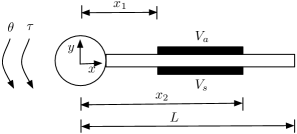
Figure 2: Schematic diagram of a slewing beam equivalent to a robotic arm.

Consider a robotic arm pinned to a motor at one end and an equivalent slewing beam model shown in Figure 2; see (Pota and Alberts,, 1995). Two piezoelectric patches are attached to the arm on either side of the beam. They act as an actuator and a sensor, respectively. The system has input voltage $V_{a}$ applied to the piezoelectric actuator and input torque $\tau$ applied by the motor. On the other hand, the outputs of the system are the voltage $V_{s}$ produced by the piezoelectric sensor and the motor hub angle $\theta$. A distributed-parameter transfer function matrix for the robotic arm is provided in (Pota and Alberts,, 1995):

$$\begin{bmatrix}{\frac{N_{\tau,\theta}(s)}{D(s)}}&{\frac{N_{V_{a},\theta}(s)}{D(s)}}\\ {\frac{N_{\tau,V_{s}}(s)}{D(s)}}&{\frac{N_{V_{a},V_{s}}(s)}{D(s)}}\end{bmatrix},$$

where $N_{\tau,\theta}$, $N_{V_{a},\theta}$, $N_{\tau,V_{s}}$, $N_{V_{a},V_{s}}$, and $D$ are given in equations (26)-(28) in (Pota and Alberts,, 1995).

By approximating the distributed-parameter model as in (Mabrok et al.,, 2014) with a first-resonant mode and ignoring the free body dynamics, one obtains

$$G(s):=\frac{1}{6.6667\times 10^{-8}}\begin{bmatrix}{\frac{3.0907}{s^{2}+3.4^{2}}+0.3}&{\frac{3.557\times 10^{-4}}{s^{2}+3.4^{2}}}\\ {\frac{3.557\times 10^{-4}}{s^{2}+3.4^{2}}}&{\frac{2.35}{s^{2}+3.4^{2}}+0.3}\end{bmatrix}.$$

Note that $G$ is negative imaginary since $j[G(j\omega)-G(j\omega)^{*}]=0$ for all $\omega\in(0,\infty)\setminus 3.4$. This follows from the fact that $G(j\omega)$ is real and symmetric for all $\omega>0$ such that $j\omega$ is not a pole of $G$. Furthermore, the residue matrix

$$\lim_{s\rightarrow j3.4}(s-j3.4)jG(s)$$

$$=\, \frac{1}{6.6667\times 10^{-8}}\begin{bmatrix}{\frac{3.0907}{6.8}+0.3}&{\frac{3.557\times 10^{-4}}{6.8}}\\ {\frac{3.557\times 10^{-4}}{6.8}}&{\frac{2.35}{6.8}+0.3}\end{bmatrix}>0.$$

To stabilise the plant $G\in\boldsymbol{\mathrm{N}}$, an integral resonant controller (IRC) (Petersen and Lanzon,, 2010) is employed. An IRC is a first-order controller taking the form

$$\bar{G}(s)=(sI+\Gamma\Phi)^{-1}\Gamma-\Delta,$$

which is strictly negative imaginary if $\Gamma>0$, $\Phi>0$ and $\Delta$ is symmetric (Petersen and Lanzon,, 2010, Thm. 8). Let

$$\Gamma :=\begin{bmatrix}{35}&{15}\\ {15}&{20}\end{bmatrix}\quad\Phi:=\begin{bmatrix}{745}&{521}\\ {521}&{1.021}\end{bmatrix}$$

$$\Delta :=\begin{bmatrix}{2.0871}&{-1.0650}\\ {-1.0650}&{1.5229}\end{bmatrix}.$$

Note that since $\bar{G}(\infty)<0$ and $G(\infty)\bar{G}(\infty)\neq 0$, (Xiong et al.,, 2010, Thm. 1) cannot be applied here to analyse the stability of the feedback interconnection $[G,\bar{G}]$. However, it can be easily verified that $\bar{\sigma}(G(0)\bar{G}(0))\approx 0$ and $\bar{\sigma}(G(\infty)\bar{G}(\infty))=0.8720<1$, whereby Corollary 10 holds and $[G,\bar{G}]$ is stable.

Suppose the feedthrough term of $\bar{G}$ is now

$$\Delta:=\begin{bmatrix}{10}&{0}\\ {0}&{10}\end{bmatrix}.$$

It follows that $\bar{\sigma}(G(0)\bar{G}(0))=3.3574\times 10^{7}$ and $\bar{\sigma}(G(\infty)\bar{G}(\infty))=3$. As such, the conditions of Corollary 10 fail to hold and hence it cannot be used to conclude stability of $[G,\bar{G}]$. However, by defining

$$\Pi_{0}=\Pi_{\infty}:=\begin{bmatrix}{0}&{I}\\ {I}&{0}\end{bmatrix},$$

it is straightforward to verify that the conditions in Theorem 8 hold. As such, $[G,\bar{G}]$ is stable. Note that the multipliers $\Pi_{0}$ and $\Pi_{\infty}$ employed in this example correspond to an IQC characterising passivity (Megretski and Rantzer,, 1997). Intuitively, the stability of $[G,\bar{G}]$ is established in this example by exploiting the fact that $\bar{G}$ and $G$ exhibit negative imaginary property at positive frequencies that are bounded away from zero and infinity, and the positive real property when the frequencies are sufficiently small or sufficiently large.

7.2 Irrational transfer functions

Consider $G=\frac{0.2}{s^{2}+1}$ and $\bar{G}=\frac{e^{-Ts}+3}{s+1}$. Observe that $\bar{G}$ contains an exponential term, which corresponds to a time-delay operation in the time domain. It is straightforward to verify that $G\in\boldsymbol{\mathrm{N}}$ and $\bar{G}\in\boldsymbol{\mathrm{N}}_{s}$ for all time delays $T\geq 0$. Furthermore, $\displaystyle\lim_{s\rightarrow j}(s-j)jG(s)=0.1>0$, $G(0)\bar{G}(0)=0.8<1$ and $G(\infty)\bar{G}(\infty)=0$ for all $T\geq 0$. Therefore, by application of Corollary 10, it follows that $[\tau G,\bar{G}]$ is stable for all $\tau\in[0,1]$ and $T\geq 0$. Note that for this example, since $\bar{G}$ is an irrational transfer function due to the presence of the time-delay term, results in (Lanzon and Petersen,, 2008; Xiong et al.,, 2010) are not applicable for concluding feedback stability.

Conversely, since it is known that $[\tau G,\bar{G}]$ is stable for all $\tau\in[0,1]$ and $T\geq 0$, it follows from Theorem 12 that there exist symmetric $\Pi_{0}$ and $\Pi_{\infty}$ such that the quadratic matrix inequalities therein hold. They can be taken, for example, to be

$$\Pi_{0}:=\begin{bmatrix}{0.8}&{0}\\ {0}&{-1}\end{bmatrix}\quad\text{and}\quad\Pi_{\infty}:=\begin{bmatrix}{0}&{0}\\ {0}&{-1}\end{bmatrix}.$$

8 Conclusions

This paper establishes necessary and sufficient conditions for robust stability of feedback interconnections of negative imaginary distributed-parameter systems using an integral quadratic constraint (IQC) approach. In contrast with the existing methods in the literature, the results were obtained without exploiting explicit state-space or transfer-function representations. Of future interest are generalisations to accommodate free body dynamics corresponding to poles at the origin (Mabrok et al.,, 2014). Nonlinear systems exhibiting counterclockwise input-output dynamics (Angeli,, 2006) may also be considered within the framework of IQCs as extensions of negative imaginary systems to nonlinear settings.

References

• Anderson and Vongpanitllerd, (2007) Anderson, B. D. O. and Vongpanitllerd, S. (2007). Network Analysis and Synthesis: A Modern Systems Theory Approach. Prentice Hall.
• Angeli, (2006) Angeli, D. (2006). Systems with counterclockwise input-output dynamics. IEEE Trans. Autom. Contr., 51(7):1130–1143.
• Bao and Lee, (2007) Bao, J. and Lee, P. L. (2007). Process Control: The Passive Systems Approach. Advances in Industrial Control. Springer.
• Bhikkaji and Moheimani, (2009) Bhikkaji, B. and Moheimani, S. O. R. (2009). Fast scanning using peizoelectric tube nanopositioners: A negative imaginary approach. In Proc. IEEE/ASME Int. Conf. Advanced Intelligent Mechatronics AIM, pages 274–279, Singapore.
• Cantoni et al., (2013) Cantoni, M., Jönsson, U. T., and Khong, S. Z. (2013). Robust stability analysis for feedback interconnections of time-varying linear systems. SIAM J. Control Optim., 51(1):353–379.
• Curtain and Zwart, (1995) Curtain, R. F. and Zwart, H. J. (1995). An Introduction to Infinite-Dimensional Linear Systems Theory. Texts in Applied Mathematics 21. Springer-Verlag.
• Das et al., (2013) Das, S. K., Pota, H. R., and Petersen, I. R. (2013). Stability analysis for interconnected systems with mixed passivity, negative-imaginary and small-gain properties. In Australian Control Conference, Perth, Australia.
• Devasia et al., (2007) Devasia, S., Eleftheriou, E., and Moheimani, S. O. R. (2007). A survey of control issues in nanopositioning. IEEE Transactions on Control Systems Technology, 15(5):802–823.
• Ferrante et al., (2015) Ferrante, A., Lanzon, A., and Ntogramatzidis, L. (2015). Foundations of not necessarily rational negative imaginary systems theory: Relations between classes of negative imaginary and positive real systems. IEEE Trans. Autom. Contr. In press.
• Ferrante and Ntogramatzidis, (2013) Ferrante, A. and Ntogramatzidis, L. (2013). Some new results in the theory of negative imaginary systems with symmetric transfer matrix function. Automatica, 49:2138–2144.
• Iwasaki and Hara, (1998) Iwasaki, T. and Hara, S. (1998). Well-posedness of feedback systems: Insights into exact robustness analysis and approximate computations. IEEE Trans. Autom. Contr., 43(5):619–630.
• Jun and Safonov, (2002) Jun, M. and Safonov, M. G. (2002). Rational multiplier IQCs for uncertain time-delays and LMI stability conditions. IEEE Trans. Autom. Contr., 47(11):1871–1875.
• Khalil, (2002) Khalil, H. K. (2002). Nonlinear Systems. Prentice Hall, 3rd edition.
• Khong et al., (2017) Khong, S. Z., Lovisari, E., and Kao, C.-Y. (2017). Robust synchronisation in multi-agent networks with unstable dynamics. IEEE Transactions on Control of Network Systems. In press.
• Khong et al., (2016) Khong, S. Z., Lovisari, E., and Rantzer, A. (2016). A unifying framework for robust synchronisation of heterogeneous networks via integral quadratic constraints. IEEE Trans. Autom. Contr., 61(5):1297–1309.
• Khong et al., (2015) Khong, S. Z., Petersen, I. R., and Rantzer, A. (2015). Robust feedback stability of negative imaginary systems: An integral quadratic constraint approach. In European Control Conference.
• Lanzon and Petersen, (2008) Lanzon, A. and Petersen, I. R. (2008). Stability robustness of a feedback interconnection of systems with negative imaginary frequency response. IEEE Trans. Autom. Contr., 53(4):1042–1046.
• Mabrok et al., (2014) Mabrok, M. A., Kallapur, A. G., Petersen, I. R., and Lanzon, A. (2014). Generalizing negative imaginary systems theory to include free body dynamics: Control of highly resonant structure with free body motion. IEEE Trans. Autom. Contr., 59(10):2692–2707.
• Megretski et al., (2010) Megretski, A., Jönsson, U. T., Kao, C.-Y., and Rantzer, A. (2010). Integral quadratic constraints. In Levine, W., editor, The Control Handbook. CRC Press (Taylor and Francis Group), second edition.
• Megretski and Rantzer, (1997) Megretski, A. and Rantzer, A. (1997). System analysis via integral quadratic constraints. IEEE Trans. Autom. Contr., 42(6):819–830.
• Petersen, (2015) Petersen, I. R. (2015). Physical interpretations of negative imaginary systems. In Proc. Asian Control Conference.
• Petersen and Lanzon, (2010) Petersen, I. R. and Lanzon, A. (2010). Feedback control of negative imaginary systems. IEEE Control System Magazine, 30(5):54–72.
• Pota and Alberts, (1995) Pota, H. R. and Alberts, T. E. (1995). Multivariable transfer functions for a slowing piezoelectric laminate beam. Journal of Dynamic Systems, Measurements and Control, 117(2):352–359.
• Scorletti, (1997) Scorletti, G. (1997). Robustness analysis with time-delays. In Proceedings of the 36th IEEE Conf. Decision Control, pages 3824–3829.
• van der Schaft, (2011) van der Schaft, A. (2011). Positive feedback interconnection of hamiltonian systems. In Proc. 50th IEEE Confence on Decision and Control and European Control Conference.
• van der Schaft, (2016) van der Schaft, A. (2016). $L_{2}$-Gain and Passivity Techniques in Nonlinear Control. Communications and Control Engineering. Springer, third edition.
• Wang et al., (2015) Wang, J., Lanzon, A., and Petersen, I. R. (2015). Robust output feedback consensus for networked negative-imaginary systems. IEEE Trans. Autom. Contr., 60(9):2547–2552.
• Xiong et al., (2010) Xiong, J., Petersen, I. R., and Lanzon, A. (2010). A negative imaginary lemma and the stability of interconnections of linear negative imaginary systems. IEEE Trans. Autom. Contr., 55(10):2342–2347.
• Zahedzadeh et al., (2008) Zahedzadeh, V., Marquez, H. J., and Chen, T. (2008). On the input-output stability of nonlinear systems: Large gain theorem. In American Control Conference.