A sparse-grid isogeometric solver

Abstract

Isogeometric Analysis (IGA) typically adopts tensor-product splines and NURBS as a basis for the approximation of the solution of PDEs. In this work, we investigate to which extent IGA solvers can benefit from the so-called sparse-grids construction in its combination technique form, which was first introduced in the early 90’s in the context of the approximation of high-dimensional PDEs.

The tests that we report show that, in accordance to the literature, a sparse-grid construction can indeed be useful if the solution of the PDE at hand is sufficiently smooth. Sparse grids can also be useful in the case of non-smooth solutions when some a-priori knowledge on the location of the singularities of the solution can be exploited to devise suitable non-equispaced meshes. Finally, we remark that sparse grids can be seen as a simple way to parallelize pre-existing serial IGA solvers in a straightforward fashion, which can be beneficial in many practical situations.

Highlights

• A sparse grid version of classical isogeometric solvers is proposed

• The proposed methodology is competitive with standard isogeometric solvers if the solution of the PDE is sufficiently smooth

• The proposed methodology can reuse pre-existing isogeometric solvers almost out-the-box and can be thought as a simple way to parallelize a serial solver

• Radical meshes in the parametric domain can be adopted as a remedy to improve sparse grid convergence for solutions without sufficient regularity on domains with corners.

1 Introduction

Isogeometric analysis (IGA), which was introduced by Hughes et al. [1, 2] in 2005, consists in solving numerically a PDE by approximating its solution with B-splines, Non-Uniform Rational B-Splines (NURBS), and extensions, i.e., with the same basis employed to parametrize the computational geometry with CAD softwares. The method has attracted considerable attention in the engineering computing community, not only because it could simplify the meshing process but also because of other interesting features, including a larger flexibility in the choice of the polynomial degree and regularity of the basis used to approximate the solution, and a more effective error vs. degrees-of-freedom ratio with respect to standard finite element methods; see [3] and references therein.

In this paper, we focus on computational cost efficiency, and in particular on the fact that $d$-dimensional splines are generated by tensorization of univariate splines, which means that the computational work typically increases exponentially with the dimension $d$ of the problem. Although this phenomenon is somehow acceptable for $d=2,3$, it could nevertheless lead to excessive computational costs both in the formation of the Galerkin matrix and in the solution of the corresponding linear system.

While a possible way out would be to embrace the tensor structure of the construction and exploit it to optimize as much as possible quadrature and linear solvers, see, e.g., [4, 5, 6, 7, 8, 9, 10, 11, 12], here we consider an alternative approach and explore the possibility of moving from a tensor grid to a so-called sparse grid, together with the combination technique.

Sparse grids emerged in the 90’s as a technique to solve generic $d$-dimensional PDEs, see [13, 14, 15, 16, 17, 18], and have shown to be quite effective in mitigating the dependence of the computational cost on $d$, if the solution features certain regularity assumptions, more demanding than the usual Sobolev ones. More precisely, denoting by $h$ the finest mesh-size of a discretization, a classic sparse-grid construction with piecewise linear polynomials only needs $\mathcal{O}(h^{-1}\log(h^{-1})^{d-1})$ degrees-of-freedom to yield an $\mathcal{O}(h^{-2}\log(h^{-1})^{d-1})$ $L^{2}$ approximation error, as opposed to a standard tensor-based approximation method which would need $\mathcal{O}(h^{-d})$ degrees-of-freedom (note the exponential dependence on $d$) for an $\mathcal{O}(h^{-2})$ $L^{2}$ approximation error, i.e. a much larger number of degrees-of-freedom for almost the same convergence rate. Roughly speaking, the sparse-grid technique consists in rewriting a tensor approximation of a function (in this work, built with tensorized splines) as a sum of hierarchical tensor contributions, and then observing that under suitable regularity assumptions the more expensive contributions (i.e., those corresponding to fine discretizations along all directions simultaneously) are actually negligible and can thus be safely neglected without compromising too much the accuracy of the approximation. Upon some rearrangment of the sparse-grid formula, the final form that will be used in practice (the so-called “combination technique”) will consist of a linear combination of a certain number of “small” tensor approximations, which will recover a close-to-full order approximation. It is important to remark that each of these tensor approximations is just a standard PDE solve (IGA in this work), which can be computed independently: therefore, sparse grids can also be seen as a straightforward way of parallelizing a legacy serial IGA solver. Note in particular that the communcation between computing cores is reduced to a minimum if one is not interested in pointwise value of the solution everywhere in the domain but rather in linear functionals of the solution.

The main goal of this work is to discuss both how IGA can take advantage of a sparse-grid construction, and vice-versa, how IGA can help broadening the field of application of the sparse-grid technique. Indeed, IGA solvers would provide a natural and systematic way of extending the sparse-grid approach, specifically by allowing use of basis functions with arbitrary degree and regularity, and general non-square domains. Note that extensions of sparse grids to these features were already proposed in literature between the mid 1990s and the early 2000s and are mentioned in the 2004 sparse-grid survey paper [17]: curvilinear domains generated by transfinite interpolation where proposed by [19, 20], while high-order hierarchicial Lagrange polynomials were analyzed in [20, 21]. Other alternatives for high-order polynomial mentioned in [17, chap. 4.5] are bicubic Hermite polynomials or higher-order finite-differences/interpolets. However, these works did not have a significant follow-up, perhaps due to the fact that they required advanced tools to generate non-standard polynomial bases, while splines-based IGA solvers are nowadays widely available and can be easily used in a combination technique formulation in a black-box fashion.

In order to improve convergence for problems with corner and edge singularities, that do not possess the Sobolev regularity that is required for optimal convergence of sparse grids, we combine sparse grids with non-uniform radical meshes, see [22, 23]. This idea was briefly touched in previous sparse grids literature in [24, 25].

The rest of this work is organized as follows: Section 2 introduces the test case considered throughout the rest of the paper and its discretization via IGA. Section 3 explains the details of the sparse-grid construction and recalls the related convergence results; observe that these are derived in the case of a square-cubic domain, but hold also in the tests in Section 4 where non-square domains are considered. Section 4 will also report the performance of the sparse grids in terms of accuracy versus computational time and number of degrees-of-freedom, over a few different geometries, and discuss the potential advantages of the sparse-grid method over a standard tensorized discretization. Concluding remarks and perspectives on future works are wrapped up in Section 5.

2 Method

2.1 Problem setting

Let $\Omega\subset\mathbb{R}^{d}$, $d=2,3$ be a compact set. In this paper, we focus on an elementary problem, i.e. the Poisson equation:

Problem 1.

Find $u:\Omega\rightarrow\mathbb{R}$ such that

$$\begin{cases}-\Delta u(\mathbf{x})=f(\mathbf{x})&\mbox{ in }\Omega\\ u(\mathbf{x})=0&\mbox{ on }\partial\Omega.\end{cases}$$ (1)

A sufficient condition for $u\in H^{k}(\Omega)$, $k\geq 1$, is that $f\in H^{k-2}(\Omega)$ and $\partial\Omega\in C^{k}(\mathbb{R}^{d-1})$. For non-smooth domains, for instance domains with corners, see e.g. [26].

2.2 The isogeometric method for solving PDEs

We now briefly recall here the fundamentals of IGA and refer to [1, 3, 27, 28] for a more thorough discussion. Given a so-called parametric interval, $\hat{I}$ (typically, $\hat{I}=[0,1]$), we introduce a knot vector, i.e, a non-decreasing vector $\Xi=[\xi_{1},\xi_{2}...,\xi_{n+p+1}]$, with $n,p\in\mathbb{N}$, and $\xi_{1},\xi_{n+p+1}$ coinciding with the extrema of $\hat{I}$; each $\xi_{i}$ is a knot and an interval $(\xi_{i},\xi_{i+1})$ having non-zero length is an element; let us further denote by number of elements as $N_{el}$. Observe that the elements need not have the same length: if that is the case, we call such length mesh-size, and denote it by $h$. A knot vector is said to be open if its first and last knot have multiplicity $p+1$. Observe that also internal nodes could have multiplicity greater than one; we define the non-decreasing vector $Z=[\zeta_{1},\ldots,\zeta_{N_{el}+1}]$ as the vector of knots of $\Xi$ without repetitions, and let $m_{i}$ the multiplicity of $\zeta_{i}$ in $\Xi$, so that $\sum_{i=1}^{N_{el}}m_{i}=n+p+1$.

Given a knot vector $\Xi$, we define the B-splines by means of the Cox-De Boor recursive formula, for $i=1,\ldots,n$:

$$\widehat{B}_{i,0}(\xi)=\begin{cases}1&\xi_{i}\leq\xi<\xi_{i+1}\\ 0&\textrm{otherwise,}\\ \end{cases}$$ (2)

$$\widehat{B}_{i,p}(\xi)=\begin{cases}\dfrac{\xi-\xi_{i}}{\xi_{i+p}-\xi_{i}}\widehat{B}_{i,p-1}(\xi)+\dfrac{\xi_{i+p+1}-\xi}{\xi_{i+p+1}-\xi_{i+1}}\widehat{B}_{i+1,p-1}(\xi),&\xi_{i}\leq\xi<\xi_{i+p+1}\\ 0,&\textrm{otherwise,}\end{cases}$$

where we adopt the convention $0/0=0$; note that the basis corresponding to an open knot vector will be interpolatory in the first and last knot. The B-splines functions are polynomials of degree $p$ and continuity $C^{p-m_{i}}$ at $\zeta_{i}$ and they form a basis of the space of splines,

$$S_{p}(\Xi,\hat{I})=\text{span}\left\{\widehat{B}_{i,p}\,,\,\,i=1,\ldots,n\right\}.$$

For $d=2$ we define the parametric domain $\widehat{\Omega}=\hat{I}\times\hat{I}$ (extension to the case $d=3$ is trivial). We consider two open knot vectors $\Xi_{1},\Xi_{2}$ with $n_{1}+p_{1}+1$ and $n_{2}+p_{2}+1$ knots respectively, the corresponding knots without repetitions $Z_{1},Z_{2}$, and the tensor products $\mathbf{\Xi}=\Xi_{1}\otimes\Xi_{2}$, $\mathbf{Z}=Z_{1}\otimes Z_{2}$; in particular, $\mathbf{Z}$ generates a cartesian mesh over $\widehat{\Omega}$ composed by $N_{el,1}\times N_{el,2}$ rectangular elements. Taking tensor products of the univariate B-splines over $\Xi_{1}$ and $\Xi_{2}$ we obtain a basis for the space of bi-variate splines,

$$S_{\mathbf{p}}(\mathbf{\Xi},\hat{\Omega})=\text{span}\{\widehat{B}_{\mathbf{i},\mathbf{p}},\mathbf{i}\leq\mathbf{n}\},$$

where $\mathbf{i}=[i_{1},i_{2}]$, $\mathbf{p}=[p_{1},p_{2}]$, $\mathbf{n}=[n_{1},n_{2}]$, $\mathbf{i}\leq\mathbf{n}\Leftrightarrow i_{1}\leq n_{1},i_{2}\leq n_{2}$, and $\widehat{B}_{\mathbf{i},\mathbf{p}}(\xi_{1},\xi_{2})=\widehat{B}_{i_{1},p_{1}}(\xi_{1})\widehat{B}_{i_{2},p_{2}}(\xi_{2})$.

We assume for the sake of simplicity that the computational domain $\Omega$ can then be parameterized by a linear combination of B-splines with given control points $\mathbf{P}_{\mathbf{i}}\in\mathbb{R}^{2}$,

$$\mathbf{x}\in\Omega\Leftrightarrow\mathbf{x}=\mathbf{F}(\bm{\xi})=\sum_{\mathbf{i}\leq\mathbf{n}}\mathbf{P}_{\mathbf{i}}\widehat{B}_{\mathbf{i},\mathbf{p}}(\bm{\xi})\text{ for some }\bm{\xi}\in\widehat{\Omega},$$ (3)

where $\mathbf{F}:\widehat{\Omega}\rightarrow\Omega$ is the parameterization of the geometry $\Omega$. For the sake of exposition, we focus in this section on B-splines, but everything can be repeated verbatim for NURBS.

According to the isogeometric principle, the spline basis is also used to approximate the solution of the Poisson equation. To this end, we introduce the spline space on the physical domain $\Omega$ as follows:

$$S_{\mathbf{p}}(\mathbf{\Xi},\Omega)=\text{span}\{B_{\mathbf{i},\mathbf{p}}=\widehat{B}_{\mathbf{i},\mathbf{p}}\circ\mathbf{F}^{-1},\mathbf{i}\leq\mathbf{n}\}$$ (4)

and then approximate the solution of Problem 1 as

$$u(\mathbf{x})\approx u_{\mathbf{n}}(\mathbf{x})=\sum_{\mathbf{i}\leq\mathbf{n}}c_{\mathbf{i}}B_{\mathbf{i},\mathbf{p}}(\mathbf{x}).$$ (5)

Much like with the finite element spaces, the isogeometric approximation of $u$ in (5), $u_{\mathbf{n}}$, converges to $u$ as the cardinality of $S_{\mathbf{p}}(\mathbf{\Xi},\Omega)$ increases. In this work, we focus on a $h$-refinement version of the sparse-grid technique, but it could be possible to devise a $p$-sparsification technique as well (or a combined $h-p$ version). In the numerical experiments in Section 4, we will consider isotropic degrees, i.e., $p_{1}=\ldots,p_{d}=p$. For a fixed degree $p$, we will consider both $C^{0}$ and $C^{p-1}$ versions of the $h$-refinement (the $C^{p-1}$ case is referred to as “$k$-refinement” or “$k$-method” in the isogeometric literature).

3 Sparse grids

The basic building block for a sparse-grid construction is a sequence of nested and increasingly accurate univariate approximation operators, which will be then first “hiercharchized” (i.e., an equivalent sequence of hierarchical operators will be derived from the initial sequence) and then tensorized.

The sequence of univariate approximation spaces/operators of a generic function $f:\hat{I}\rightarrow\mathbb{R}$, indexed by $\alpha\in\mathbb{N}\cup\{0\}$, is constructed as follows. We first introduce the trivial open knot vector over the reference interval $\hat{I}$, $\Xi_{0}=[0,\ldots,0,1,\ldots,1]$, and generate the $\alpha$-th open knot vector $\Xi_{\alpha}$ by dyadic subdivision of $\Xi_{0}$, so that $\Xi_{\alpha}$ has $2^{\alpha}$ elements. For notational convenience, we then denote by the short-hand $S_{\alpha}$ the space of B-splines/NURBS built over $\Xi_{\alpha}$ with fixed degree $p=1,2,3$, i.e., $S_{\alpha}=S_{p}(\Xi_{\alpha},\hat{I})$, and $f_{\alpha}$ be a suitable approximation of $f$ in $S_{\alpha}$ (later, a Galerkin approximation). Finally, the univariate “hierarchization” of the sequence of approximation is obtained by defining the operators

$$\Delta_{\alpha}(f)=f_{\alpha}-f_{\alpha-1},$$

where we adopt the convention $f_{-1}=0$. Observe that the following telescopic equality holds:

$$f_{\alpha}=\sum_{k=0}^{\alpha}\Delta_{k}(f).$$

As for the second step (the “tensorization”) we again illustrate it in $d=2$, for ease of notation, but the construction can be applied with straightforward modifications to any $d$. Thus, let now $f:\hat{I}_{1}\otimes\hat{I}_{2}=\widehat{\Omega}\rightarrow\mathbb{R}$ and consider a multi-index with non-negative components $\bm{\alpha}=[\alpha_{1},\,\alpha_{2}]\in(\mathbb{N}\cup\{0\})^{2}$. Furthermore, let $\mathbf{\Xi}_{\bm{\alpha}}=\Xi_{\alpha_{1}}\times\Xi_{\alpha_{2}}$, and the corresponding B-splines space be $S_{\bm{\alpha}}$. Extending the univariate notation, we now let $f_{\bm{\alpha}}$ be the approximation of $f$ in $S_{\bm{\alpha}}$, and in particular we denote by $f_{[\alpha_{1},\infty]},f_{[\infty,\alpha_{2}]}$ the semi-discrete approximations of $f$ along directions $\xi_{1}$ and $\xi_{2}$. We then consider hierarchical operators along each direction individually, i.e., let

$$\Delta^{1}_{\alpha_{1}}f=f_{[\alpha_{1},\infty]}-f_{[\alpha_{1}-1,\infty]},$$

be the difference of two consecutive semi-discrete approximations of $f$ along direction $\xi_{1}$, and analogously

$$\Delta^{2}_{\alpha_{2}}f=f_{[\infty,\alpha_{2}]}-f_{[\infty,\alpha_{2}-1]},$$

and we introduce the multidimesional hierachical operator as the tensor product of the univariate $\Delta_{\alpha}$ operators, i.e.,

$$\Delta_{\bm{\alpha}}(f) =\Delta^{1}_{\alpha_{1}}[\Delta^{2}_{\alpha_{2}}(f)]$$ (6)

$$=\Delta^{1}_{\alpha_{1}}[f_{[\infty,\alpha_{2}]}-f_{[\infty,\alpha_{2}-1]}]$$

$$=f_{[\alpha_{1},\alpha_{2}]}-f_{[\alpha_{1}-1,\alpha_{2}]}-f_{[\alpha_{1},\alpha_{2}-1]}+f_{[\alpha_{1}-1,\alpha_{2}-1]},$$ (7)

where the last form is usually referred to as the combination technique. Observe that by telescopy

$$f_{\bm{\alpha}}=\sum_{\bm{\beta}\leq\bm{\alpha}}\Delta_{\bm{\beta}}(f).$$ (8)

Upon introducing this hierarchical decomposition of the approximation of $f$, the crucial observation is that for $f$ regular enough the norm of each component $\Delta_{\bm{\beta}}(f)$ can be expected to be decreasing with respect to $|\bm{\beta}|=\sum_{\ell=1}^{d}\beta_{\ell}$. If that is the case, many of the terms in (8) can be dismissed from the approximation without compromising too much its accuracy. At the same time however, due to the dyadic subdivision approach used to generate the univariate spaces $S_{\alpha}$ to be tensorized, it can be easily seen from (7) that the number of degrees-of-freedom of $\Delta_{\bm{\beta}}$ grows exponentially in $|\bm{\beta}|=\sum_{\ell=1}^{d}\beta_{\ell}$. Thus, introducing

$$f_{J}=\sum_{|\bm{\beta}|\leq J}\Delta_{\bm{\beta}}(f),\quad\text{for some }J\in\mathbb{N}\cup\{0\},$$ (9)

we are left with an approximation which gives up moderately on the accuracy while, in fact, significantly reducing the number of degrees-of-freedom. Observe that in principle, such a computation can be already performed by considering the sparse-grid approximation in the form of (9); however, this requires using discretizations of hierarchical type, which may not be straightforward. Instead, by further expanding each $\Delta_{\bm{\beta}}$ in (9) as in (7), we obtain the following expression of the sparse-grid approximation (see [29, Lemma 1] for the derivation of the expression) which is more amenable to computation, because it only employs standard solvers:

$$f_{J} =\sum_{\mathbf{k}\in\{0,1\}^{d},|\bm{\beta}+\mathbf{k}|\leq J}(-1)^{|\mathbf{k}|}f_{\bm{\beta}}$$ (10)

$$=\sum_{J-d+1\leq|\bm{\beta}|\leq J}(-1)^{J-|\bm{\beta}|}\binom{d-1}{J-|\bm{\beta}|}f_{\bm{\beta}}$$ (11)

$$=\begin{cases}\displaystyle\sum_{|\bm{\beta}|=J}f_{\bm{\beta}}-\sum_{|\bm{\beta}|=J-1}f_{\bm{\beta}}&\text{if }d=2,\\[12.0pt] \displaystyle\sum_{|\bm{\beta}|=J}f_{\bm{\beta}}-2\sum_{|\bm{\beta}|=J-1}f_{\bm{\beta}}+\sum_{|\bm{\beta}|=J-2}f_{\bm{\beta}}&\text{if }d=3,\end{cases}$$ (12)

where the derivation of the second equality can be found in, e.g., [29]. We refer to (10) as the combination technique form of $f_{J}$, see, e.g., [16, 30, 31, 32, 18, 33, 34]. We remark that the number of components to be computed in the combination technique (10) is substantially smaller than the number of hierarchical components in (9): indeed, the set in (9) is a discrete simplex while in (10) only the uppermost $d$ layers of such simplex need to be computed. More precisely:

• for $d=2$ one has $\mathrm{card}\big{(}\{|\bm{\beta}|\leq J\}\big{)}=\frac{J(J+1)}{2}=\mathcal{O}(J^{2})$ while $\mathrm{card}\big{(}\{|\bm{\beta}|=J\}\big{)}+\mathrm{card}\big{(}\{|\bm{\beta}|=J-1\}\big{)}=2J-1=\mathcal{O}(J)$;

• for $d=3$ one has $\mathrm{card}\big{(}\{|\bm{\beta}|\leq J\}\big{)}=\frac{J(J+1)(J+2)}{6}=\mathcal{O}(J^{3})$ while $\mathrm{card}\big{(}\{|\bm{\beta}|=J\}\big{)}+\mathrm{card}\big{(}\{|\bm{\beta}|=J-1\}\big{)}+\mathrm{card}\big{(}\{|\bm{\beta}|=J-2\}\big{)}=\frac{2}{3}J(J-1)+1=\mathcal{O}(J^{2})$.

In practice, computing $f_{J}$ entails solving a number of “moderate” tensor approximations of $f$ where the $d$ directions are never simultaneously refined to full accuracy, compared to the full tensor approximation $f_{\bm{\alpha}}$ (see also Example 1 detailed next). The quantity $h$ appearing in the estimates below is defined as $h=2^{-J}$ and is proportional to the finest mesh-size employed in the sparse-grid discretization (which, we recall again, is never reached “simultaneously” along each direction). A combination technique formula uses $\mathcal{O}(J^{d-1}2^{J})=\mathcal{O}(h^{-1}|\log_{2}h|^{d-1})$ degrees of freedom, see, e.g., [20, 21], compared to the corresponding fully resolved grid that employs $\mathcal{O}(2^{Jd})=\mathcal{O}(h^{-d})$ degrees of freedom. Crucially, note that the number of degrees of freedom of the sparse grid depends in a milder way on $d$.

Figure 1: Bezier meshes for Example 1. From left to right: $f_{[0\,0]}$, $f_{[1\,0]}$, $f_{[0\,1]}$, $f_{[1\,1]}$. The first three are to be linearly combined as in Equation (13) to obtain the combination technique, to be contrasted with the last full approximation grid.

Example 1.

In this example we consider $\hat{I}=[0,1]$, the knot-vector $\Xi_{0}=[0,0,1,1]$, and $\widehat{\Omega}=[0,1]^{2}=\hat{I}\otimes\hat{I}$. We then consider an approximation of $f:\widehat{\Omega}\rightarrow\mathbb{R}$ with a sparse grid using $J=1$, and below we show the calculus to convert the sparse-grid representation of $f_{J}$, (9), to its combination technique equivalent, (10).

$$f_{J}=\sum_{\beta_{1}+\beta_{2}\leq J=1}\Delta_{\bm{\beta}}(f) =\Delta_{[1,0]}(f)+\Delta_{[0,1]}(f)+\Delta_{[0,0]}(f)$$

$$=f_{[1,0]}-f_{[0,0]}-\underbrace{f_{[1,-1]}}_{0}+\underbrace{f_{[0,-1]}}_{0}$$

$$+f_{[0,1]}-\underbrace{f_{[-1,1]}}_{0}-f_{[0,0]}+\underbrace{f_{[-1,0]}}_{0}$$

$$+f_{[0,0]}-\underbrace{f_{[-1,0]}}_{0}-\underbrace{f_{[0,-1]}}_{0}+\underbrace{f_{[-1,-1]}}_{0}$$

$$=f_{[1,0]}+f_{[0,1]}-f_{[0,0]}.$$ (13)

Observe also that by adding the operator $\Delta_{[1,1]}(f)$ to the sparse-grid representation above, we obtain the full tensor approximation $f_{[1,1]}$, in agreement with the telescopic formula (8):

$$f_{J}+\Delta_{[1,1]}(f)=\sum_{[\beta_{1},\beta_{2}]\leq[1,1]}\Delta_{\bm{\beta}}(f) =\Delta_{[1,1]}(f)+f_{[1,0]}+f_{[0,1]}-f_{[0,0]}$$

$$=f_{[1,1]}-f_{[0,1]}-f_{[1,0]}+f_{[0,0]}+f_{[1,0]}+f_{[0,1]}-f_{[0,0]}$$

$$=f_{[1,1]}.$$ (14)

The results are illustrated in Figure 1. The meshes of the three components of $f_{J=1}$ in (13) are the three left-most meshes, while the right-most mesh is the one of the full tensor grid approximation $f_{[1,1]}$. It is evident how the full resolution $h=1/2$ is reached only in one direction at a time for the combination technique.

Finally, we discuss the convergence of the combination technique, following closely [32, 35, 36]; see also [30, 33, 37, 38]. Note that, although the sparse-grid representation (9) and the combination technique (10) are formally two different representations of the same approximation, the strategies to prove convergence of the two techniques are different, see, e.g., [17] and [32]. To state the convergence results, we need to introduce the so-called mixed regularity Sobolev spaces.

First, let $H^{l}(\hat{I})$ for $l\in\mathbb{R}_{+}\setminus\mathbb{N}$ be the fractional order Sobolev space, extending the definition of a standard Sobolev space $H^{l}(\hat{I})$ for integer $l$. Then, borrowing notation from [32], we define the Sobolev spaces of mixed derivatives on $\widehat{\Omega}=[0,1]^{d}$ as

$$H^{r_{1},\ldots,r_{d}}_{mix}(\widehat{\Omega})=H^{r_{1}}(\hat{I})\otimes\cdots\otimes H^{r_{d}}(\hat{I}),$$

and finally the spaces

$$\mathcal{H}_{mix}^{r_{1},\ldots,r_{d}}(\widehat{\Omega})=H^{r_{1}+1,r_{2},\ldots,r_{d}}_{mix}(\widehat{\Omega})\cap H^{r_{1},r_{2}+1,r_{3}\ldots,r_{d}}_{mix}(\widehat{\Omega})\cap\ldots\cap H^{r_{1},r_{2},\ldots,r_{d-1},r_{d}+1}_{mix}(\widehat{\Omega}).$$

As will be detailed below, the estimate of the $H^{1}$ norm of the error will be valid provided that $u$ belongs to certain $\mathcal{H}_{mix}^{r_{1},\ldots,r_{d}}$ spaces, while the estimate of the $L^{2}$ norm of the error will require $H^{r_{1},\ldots,r_{d}}_{mix}$ regularity. However, it is usually not trivial to perform a sharp mixed regularity analysis of the solution of a PDE. Thus, in the following we will also state the convergence results in terms of the standard Sobolev spaces. To this end, observe that the following inclusions trivially hold

$$H^{k}(\widehat{\Omega})\subset H^{k/d,k/d,\ldots,k/d}_{mix}(\widehat{\Omega})$$ (15)

$$H^{1+k}(\widehat{\Omega})\subset\mathcal{H}_{mix}^{k/d,k/d,\ldots,k/d}(\widehat{\Omega}).$$

In case of $C^{0}$ finite elements (though the case of higher continuity is similar), the convergence results that we report in the following have been proved for non-tensor operators on rectangular domains, i.e., on $\widehat{\Omega}$, and are valid under certain additional technical assumptions (see [32] for details on the proof of the $H^{1}$ convergence, while the proof of the $L^{2}$ convergence is detailed in [35]). Given the exploratory nature of this work, we will not try to prove the same kind of result in generic domains $\Omega=\mathbf{F}(\widehat{\Omega})$, and instead we will content ourselves with verifying numerically that these convergence rates are valid also in this latter framework.

$H^{1}$ norm

For $0<s\leq p$ there holds

$$\|u-u_{J}\|_{H^{1}(\widehat{\Omega})}\leq h^{s}J^{(d-1)/2}\|u\|_{\mathcal{H}_{mix}^{s,\ldots,s}(\widehat{\Omega})}.$$ (16)

Observe that using the inclusions in (15), it holds also that

$$\|u-u_{J}\|_{H^{1}(\widehat{\Omega})}\leq h^{s}J^{(d-1)/2}\|u\|_{H^{1+ds}(\widehat{\Omega})}.$$ (17)

Comparing the last equation with the convergence estimate of standard tensor methods

$$\|u-u_{[J,\ldots,J]}\|_{H^{1}(\widehat{\Omega})}\leq h^{s}\|u\|_{H^{1+s}},$$ (17-bis)

we see in a more quantitative way the fact that sparse grids reach the same convergence rate than standard tensor methods (up to a logarithmic term) by employing less degrees of freedom, at the expense of higher regularity requirements.

$L^{2}$ norm

For $0<s\leq r=p+1$ there holds

$$\|u-u_{J}\|_{L^{2}(\widehat{\Omega})}\leq h^{s}J^{(d-1)/2}\|u\|_{H^{s,\ldots,s}_{mix}\widehat{\Omega}},$$ (18)

and again from (15),

$$\|u-u_{J}\|_{L^{2}(\widehat{\Omega})}\leq h^{s}J^{(d-1)/2}\|u\|_{H^{sd}(\widehat{\Omega})},$$ (19)

to be compared to the standard tensor convergence

$$\|u-u_{[J,\ldots,J]}\|_{L^{2}(\widehat{\Omega})}\leq 2^{-Js}\|u\|_{H^{s}},$$ (19-bis)

leading to same conclusions as in the $H^{1}$ case.

We summarize the expected convergence rates in Table 1. Observe that, with a slight abuse, in Table 1 and in the rest of this work we use the expression “sparse-grid convergence rate” to indicate $s$, i.e. the exponent of $h$ at the right-hand side of Equations (16) to (19), neglecting the factor $J^{(d-1)/2}$ which depends logarithmically on $h$. Moreover, here and in the rest of the manuscript, we will denote by “SG-IGA” the sparse-grid version of isogeometric analysis.

$H^{1}$ error, $d=2$
	$u\in H^{2}$	$u\in H^{3}$	$u\in H^{4}$	$u\in H^{5}$	$u\in H^{6}$	$u\in H^{7}$
	($u\in\mathcal{H}_{mix}^{1/2,1/2}$)	($u\in\mathcal{H}_{mix}^{1,1}$)	($u\in\mathcal{H}_{mix}^{3/2,3/2}$)	($u\in\mathcal{H}_{mix}^{2,2}$)	($u\in\mathcal{H}_{mix}^{5/2,5/2}$)	($u\in\mathcal{H}_{mix}^{3,3}$)
$p=1$, SG-IGA	1/2	1	1	1	1	1
$p=1$, IGA	1	1	1	1	1	1
$p=2$, SG-IGA	1/2	1	3/2	2	2	2
$p=2$, IGA	1	2	2	2	2	2
$p=3$, SG-IGA	1/2	1	3/2	2	5/2	3
$p=3$, IGA	1	2	3	3	3	3

$L^{2}$ error, $d=2$
	$u\in H^{2}$	$u\in H^{3}$	$u\in H^{4}$	$u\in H^{5}$	$u\in H^{6}$	$u\in H^{7}$
	($u\in H^{1,1}$)	($u\in H^{3/2,3/2}$)	($u\in H^{2,2}$)	($u\in H^{5/2,5/2}$)	($u\in H^{3,3}$)	($u\in H^{7/2,7/2}$)
$p=1$, SG-IGA	1	3/2	2	2	2	2
$p=1$, IGA	2	2	2	2	2	2
$p=2$, SG-IGA	1	3/2	2	5/2	3	3
$p=2$, IGA	2	3	3	3	3	3
$p=3$, SG-IGA	1	3/2	2	5/2	3	7/2
$p=3$, IGA	2	3	4	4	4	4

$H^{1}$ error, $d=3$
	$u\in H^{2}$	$u\in H^{3}$	$u\in H^{4}$	$u\in H^{5}$	$u\in H^{6}$	$u\in H^{7}$
	($u\in\mathcal{H}_{mix}^{1/3,1/3,1/3}$)​​​​​​​​​	($u\in\mathcal{H}_{mix}^{2/3,2/3,2/3}$)​​​​​​​​​	($u\in\mathcal{H}_{mix}^{1,1,1}$)​​​​​​​​​	($u\in\mathcal{H}_{mix}^{4/3,4/3,4/3}$)​​​​​​​​​	($u\in\mathcal{H}_{mix}^{5/3,5/3,5/3}$)​​​​​​​​​	($u\in\mathcal{H}_{mix}^{2,2,2}$)
$p=1$, SG-IGA	1/3	2/3	1	1	1	1
$p=1$, IGA	1	1	1	1	1	1
$p=2$, SG-IGA	1/3	2/3	1	4/3	5/3	2
$p=2$, IGA	1	2	2	2	2	2
$p=3$, SG-IGA	1/3	2/3	1	4/3	5/3	2
$p=3$, IGA	1	2	3	3	3	3

$L^{2}$ error, $d=3$
	$u\in H^{2}$	$u\in H^{3}$	$u\in H^{4}$	$u\in H^{5}$	$u\in H^{6}$	$u\in H^{7}$
	($u\in H^{2/3,2/3,2/3}$)​​​​​​​​​	($u\in H^{1,1,1}$)​​​​​​​​​	($u\in H^{4/3,4/3,4/3}$)​​​​​​​​​	($u\in H^{5/3,5/3,5/3}$)​​​​​​​​​	($u\in H^{2,2,2}$)​​​​​​​​​	($u\in H^{7/3,7/3,7/3}$)
$p=1$, SG-IGA	2/3	1	4/3	5/3	2	2
$p=1$, IGA	2	2	2	2	2	2
$p=2$, SG-IGA	2/3	1	4/3	5/3	2	7/3
$p=2$, IGA	2	3	3	3	3	3
$p=3$, SG-IGA	2/3	1	4/3	5/3	2	7/3
$p=3$, IGA	2	3	4	4	4	4

Table 1: Provable lower bounds on the $H^{1}$ and $L^{2}$ convergence rates for sparse-grid (SG-IGA) and tensor approximation (IGA) and $d=2,3$.

4 Numerical tests

In what follows, we consider a few variations of Problem 1, which highlight the features of SG-IGA. More specifically, two different geometries are considered, the classical quarter of annulus in $d=2,3$ and a horseshoe-shaped domain, see Figure 2. We verify numerically that SG-IGA attains for problems with regular and low-regular solutions the theoretical convergence rates presented in Table 1, and compare SG-IGA to standard IGA in terms of computational cost. All tests have been performed using the Matlab/Octave IGA package GeoPDEs [39], on a Linux workstation with 12 i7 cores at 3.30 GHz (although all tests reported have been executed in serial unless explicitely mentioned), 64 GB RAM and Matlab 2015a 8.5.

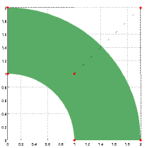
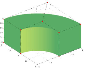
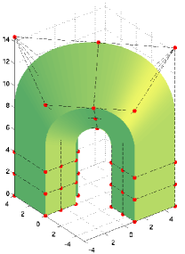
Figure 2: Domains for the numerical tests with control points (in red). Left: Quarter of annulus, $d=2$; center: quarter of annulus $d=3$; right: horseshoe.

4.1 A matter of costs

In our experiments we adopt GeoPDEs 3.0 [39], which is an isogeometric solver based on a finite element architecture. Denoting by $N_{\mathsf{EL}}$ and $N_{\mathsf{DOF}}$ the number of mesh elements and degrees-of-freedom, respectively, the standard matrix formation requires ${O(N_{\mathsf{EL}}p^{3d})}$ FLOPs for degree $p$ splines, any continuity (that is, ${O(N_{\mathsf{DOF}}p^{2d})}$ FLOPs for $C^{0}$ Bernstein polynomials and ${O(N_{\mathsf{DOF}}p^{3d})}$ FLOPs for $C^{p-1}$ splines). The linear solver cost for preconditioned iterative solvers is proportional to $N_{\mathsf{DOF}}$ but robustness with respect to $p$ is difficult or costly to achieve with standard finite element preconditioners. For small systems, a direct solver (that we adopt) is faster. Recent approaches have significantly improved computational efficiency, especially for $C^{p-1}$ continuity (see e.g. [8, 9, 7, 12, 40]).

In this work, we relate the error both to the computational time (with GeoPDEs based routines) and to the number of degrees-of-freedom: time measures the “actual cost” of our implementation (mainly dependent on the element number and polynomial degree, independent on the spline regularity), while degrees-of-freedom represent the “best” possible computational cost in an ideal setting.

When considering degrees-of-freedom as a measure of the computational cost, we remark that the components in the combination technique formula of SG-IGA are solved separately, and so, we find it of interest to look at both the largest component’s degrees-of-freedom, and the sum of all degrees-of-freedom. In fact, when fully exploiting parallelization the component with the largest degrees-of-freedom is the computational bottleneck in SG-IGA, as the combination technique is “embarrassingly parallel,” see, e.g., [15, 41, 42, 43], and one can exploit that existing IGA solvers can be used out-of-the-box.

The combination technique has two evident drawbacks: first, determining the optimal balance of its components over the cores at hand is a combinatoric problem, which is non-trivial to solve (see [42, 43] for more details on an efficient implementation of a combination technique strategy, as well as [44] for jointly optimizing both the distribution of componentes over the available cores and the use of multiple cores, i.e., employing a parallel solver, for computing a single component). Second, the approximation of the solution on the entire domain is not available unless all grids have been combined together, e.g., interpolated on a reference grid, which will have in general a non-negligible computational cost. Such a “post-process” step can be avoided if one is only interested in a linear functional of the solution.

As for the computational time, we show timings for both serial and parallel execution over $C$ cores. The time for serial execution will be the true computational time while the time for parallel executions will not be the true one but instead an “optimized time”: after having clocked the computational time for each tensor during the serial execution, we sort the tensors needed for each SG-IGA level in decreasing computational time, and assign them to the $C$ cores at disposal in this order, in such a way that as soon as a core is free it takes up the largest tensor not assigned yet. The rationale is to show the “ideal” behaviour of the combination technique by factoring out implementation suboptimalities. Furthermore, the computational time is measured as the sum of setup time (meshing and preliminary operations, including matrix and right hand side assembly) and solve time, i.e., in our results we do not consider the time it takes to evaluate the solution on the reference grid used to compute the error, which in a suboptimal implementation may dominate any other cost, for both IGA and SG-IGA.

4.2 Quarter of annulus domains, regular solution

With reference to Equation (1), we first look at the quarter-of-annulus benchmark, in its two- and three-dimensional versions. In the following, $x,y,z$ will as usual denote the components of the $d$-dimensional vector $\mathbf{x}\in\Omega$. In this first set of experiments, we choose $f(\mathbf{x})$ such that

$$u(x,y) =-(x^{2}+y^{2}-1)(x^{2}+y^{2}-4)xy^{2} \mbox{ for }d=2,$$

$$u(x,y,z) =-(x^{2}+y^{2}-1)(x^{2}+y^{2}-4)xy^{2}\sin(\pi z) \mbox{ for }d=3.$$

	$d=2$		$d=3$
	$H^{1}$ error	$L^{2}$ error	$H^{1}$ error	$L^{2}$ error
$C^{0},p=2$, SG-IGA	2.29(2)	3.03(3)	2.38(2)	3.12(3)
$C^{0},p=2$, IGA	2.10(2)	2.96(3)	2.05(2)	2.97(3)
$C^{1},p=2$, SG-IGA	2.16(2)	3.04(3)	2.23(2)	3.08(3)
$C^{1},p=2$, IGA	2.10(2)	3.00(3)	2.03(2)	3.08(3)
$C^{0},p=3$, SG-IGA	3.21(3)	3.94(4)	3.30(3)	4.00(4)
$C^{0},p=3$, IGA	3.08(3)	3.98(4)	3.06(3)	4.01(4)
$C^{1},p=3$, SG-IGA	3.05(3)	3.93(4)	3.13(3)	3.93(4)
$C^{1},p=3$, IGA	2.91(3)	3.98(4)	2.89(3)	3.85(4)
$C^{2},p=3$, SG-IGA	3.06(3)	4.15(4)	3.15(3)	4.26(4)
$C^{2},p=3$, IGA	2.93(3)	4.08(4)	2.98(3)	4.13(4)

Table 2: Convergence of SG-IGA and IGA methods with respect to the sparse-grid level, $J$. The number in parenthesis indicates the expected rate from theory, cf. Table 1.

We start the discussion by examining the convergence of the SG-IGA and IGA approximation errors in $L^{2}$ and $H^{1}$ norm with respect to the sparse-grid level $J$, cf. Equations (16) to (19). The measured numerical rates (recall the “informal definition” of sparse-grid rate we gave while discussing Table 1, at the end of Section 3) are reported in Table 2 and should be compared to Table 1, which lists the theoretical convergence rates. Numerical rates are computed by using a least squares fit (Matlab command polyfit) of the quantities in equations (17) and (19). For convenience, we complement Table 2 by indicating in parenthesis, next to each measured rate, the corresponding theoretical value taken from Table 1.

The observed SG-IGA convergence rates agree well with the theoretical ones given in the parentheses. In some cases, the resulting rates are even greater than expected: this is consistent with the observation in [32] that reports that sparse methods can achieve the same convergence behaviour as standard tensor methods, (i.e., the estimate without the correction term $J^{(d-1)/2}$ in Equations (16) to (19) holds true) when the function has some additional regularity. Some of the convergence figures from which the rates in Table 2 are deduced are shown in Figure 3. The solid lines are the $H^{1}$ and $L^{2}$ errors computed with respect to the analytical solution, and the dashed lines are the corresponding theoretical slopes given in Table 1.

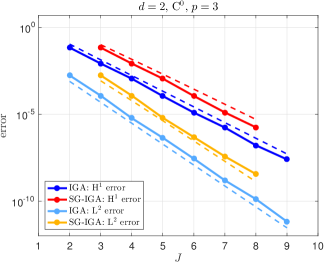
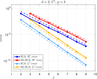
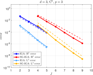
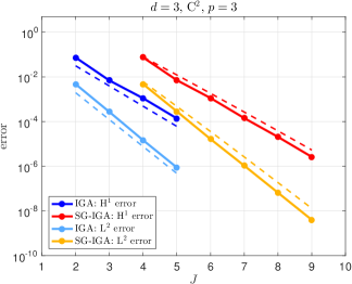
Figure 3: Error versus grid level for the problem on a quarter of annulus domain with regular solution, for $p=3$ and different values of $d$ (top row: $d=2$, bottom row: $d=3$) and of the regularity of the B-splines basis (left column: $C^{0}$, right column: $C^{2}$). The solid lines are the errors computed against the analytical solution, and the dashed lines show the corresponding theoretical rates.

The error versus computational time is shown in Figure 5: here we only show the case $p=3$ with minimal and maximal regularity for brevity. We can see that SG-IGA is an effective alternative to the standard IGA for this problem: for $d=2$, this is especially true in the multi-core situation when 4 or more cores are used, while in the case $d=3$ even using one core gives clear advantages. The dashed line indicates the lower bound on the computational cost that can be achieved if the number of available cores is at least equal to the number of components of the combination technique to be computed (such number is shown to the left in green boxes). The gain in computational effort is evident also if we consider the number of degrees-of-freedom as a computational cost indicator, cf. Figure 5. In contrast to the dashed line in the error vs. time, the dashed line here is the number of the degrees-of-freedom for the largest tensor grid in the combination technique.

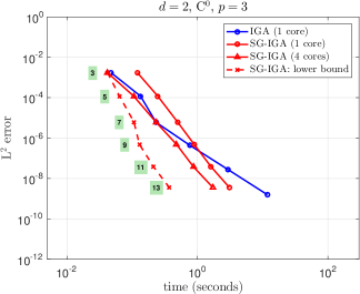
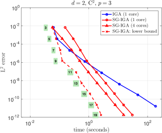
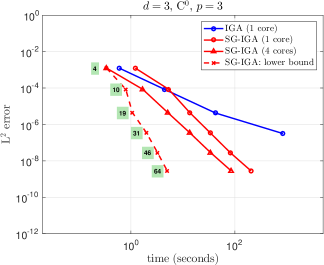
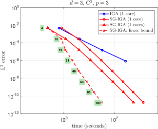
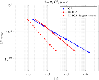
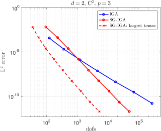
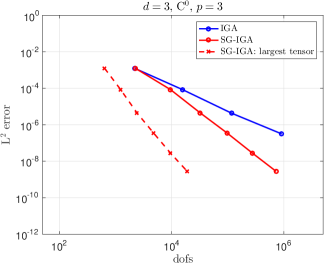
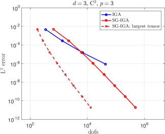
Figure 4: $L^{2}$ error vs. time for the problem on a quarter of annulus domain with regular solution. Here we fix $p=3$ and change $d$ (top row: $d=2$, bottom row: $d=3$) and the regularity of the B-splines basis (left column: $C^{0}$, right column: $C^{2}$). The dashed line is the lower bound that can be achieved if the number of available cores is at least equal to the number of components of the combination technique for each level, given by the numbers in green boxes.

Figure 5: $L^{2}$ error vs. dofs for the problem on a quarter of annulus domain with regular solution. Here we fix $p=3$ and change $d$ (top row: $d=2$, bottom row: $d=3$) and the regularity of the B-splines basis (left column: $C^{0}$, right column: $C^{2}$). In each figure, the dashed line represents the error of SG-IGA vs. the number of the degrees-of-freedom for the largest tensor grid in the combination technique.

Finally, we give for this test problem a computational validation of the truncation procedure that led to defining the sparse-grid approximation (9), which we now revisit. To obtain (9), we first introduced the decomposition of a full tensor IGA approximation $u_{[J,\ldots,J]}$ as

$$u_{[J,\ldots,J]}=\sum_{\bm{\beta}\in\mathcal{I}_{J,\text{IGA}}}\Delta_{\bm{\beta}}(u),\quad\mathcal{I}_{J,\text{IGA}}=\{\bm{\beta}\in\mathbb{R}^{d}:\max_{\kappa=1,\ldots,d}\beta_{\kappa}\leq J\},$$

cf. Equations (6) to (8), and then “pruned” the set $\mathcal{I}_{J,\text{IGA}}$ to obtain

$$u_{J}=\sum_{\bm{\beta}\in\mathcal{I}_{J,\text{SG-IGA}}}\Delta_{\bm{\beta}}(u),\quad\mathcal{I}_{J,\text{SG-IGA}}=\Big{\{}\bm{\beta}\in\mathbb{R}^{d}:\sum_{\kappa=1}^{d}\beta_{\kappa}\leq J\Big{\}},$$

under the assumption that the magnitude of $\|\Delta_{\bm{\beta}}(u)\|_{L^{2}(\Omega)}$ would be decreasing with respect to $\sum_{\kappa=1}^{d}\beta_{\kappa}$. One may therefore set up an optimization problem, and look for the best set $\mathcal{I}$, i.e., the set that delivers the best approximation of $u$ for a given computational budget,

$$\min_{\mathcal{I}\subset\mathbb{N}^{d}}\|u-u_{\mathcal{I}}\|_{L^{2}(\Omega)},$$

$$\text{such that}\quad u_{\mathcal{I}}=\sum_{\bm{\beta}\in\mathcal{I}}\Delta_{\bm{\beta}}(u)$$

$$\quad\quad\quad\quad\sum_{\bm{\beta}\in\mathcal{I}}\text{degrees-of-freedom}(\Delta_{\bm{\beta}}(u))\leq K.$$

This is a classic “knapsack” optimization problem [45] and can be approximately solved by the so-called Dantzig method:

1. define a “revenue” and a “cost” for each item that can be picked;

2. define the “profit” for each item, by taking the ratio of “revenue” over “cost”;

3. sort items according to profit in decreasing order;

4. pick up items according to the ordering just introduced, until the sum of their costs exceeds the budget constraint.

In our case, the cost of a $\Delta_{\bm{\beta}}(u)$ would be the number of degrees-of-freedom and the revenue would be its $L^{2}$ norm, which quantifies how much the sparse-grid approximation $u_{\mathcal{I}}$ would improve if $\Delta_{\bm{\beta}}(u)$ was added to the sparse-grid approximation. If one had a-priori estimates on the decay/growth of cost and revenue, one could then devise the “optimal” sparse-grid approximation for a fixed cost, see [17, 46, 47] for more details. Observe that we can compute cost and revenue for every $\Delta_{\bm{\beta}}(u)$ with $\bm{\beta}$ in a sufficiently large set, cf. Equation (6) and (7). The results of this computation for the two-dimensional quarter-of-annulus problem are reported in Figure 6, where each dot represents a multi-index $\bm{\beta}$ in the plane $(\beta_{1},\beta_{2})$, and dots are colored according to the value of their associated profit. It is clearly visible that indices with $\beta_{1}+\beta_{2}=constant$ have profit of equal magnitude, which means that they should be picked together in the approximation, thus obtaining exactly the sparse-grid expression (9). This will no longer be the case for the next numerical test.

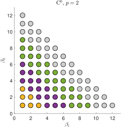
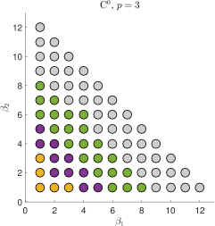
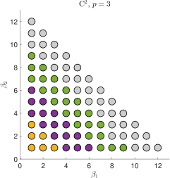
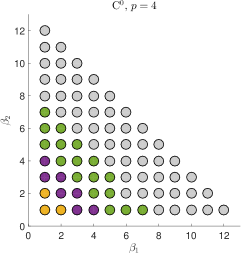
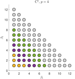
Figure 6: optimal sets for the quarter-of-annulus problem with regular solution. From top to bottom row: $p=2,3,4$. Left column: $C^{0}$ B-spline basis; Right column: maximal continuity B-splines basis.

4.3 Quarter of annulus domains, low-regular solution

	$d=2$		$d=3$
	$H^{1}$ error	$L^{2}$ error	$H^{1}$ error	$L^{2}$ error
$C^{0},p=2$, SG-IGA	1.35(1)	1.72(1.5)	1.30(2/3)	1.62(1)
$C^{0},p=2$, IGA	2.11(2)	2.71(3)	1.84(2)	2.70(3)
$C^{1},p=2$, SG-IGA	1.20(1)	1.72(1.5)	1.22(2/3)	1.63(1)
$C^{1},p=2$, IGA	2.02(2)	2.82(3)	1.81(2)	2.88(3)
$C^{0},p=3$, SG-IGA	1.26(1)	1.74(1.5)	1.30(2/3)	1.71(1)
$C^{0},p=3$, IGA	2.21(2)	3.00(3)	2.21(2)	2.89(3)
$C^{1},p=3$, SG-IGA	1.25(1)	1.78(1.5)	1.28(2/3)	1.75(1)
$C^{1},p=3$, IGA	2.14(2)	3.05(3)	2.15(2)	2.90(3)
$C^{2},p=3$, SG-IGA	1.19(1)	1.58(1.5)	1.20(2/3)	1.55(1)
$C^{2},p=3$, IGA	2.21(2)	2.92(3)	2.12(2)	2.81(3)

Table 3: Convergence of SG-IGA and IGA methods with respect to the sparse-grid level, $J$ for the low-regular problem. The number in parenthesis indicates the expected rate from theory, cf. Table 1.

In this second set of experiments we consider again the quarter-of-annulus domain, but we choose as forcing term in Equation (1) the function $f(\mathbf{x})=1$. This implies that the solution, $u$, will have limited regularity due to corner and edge singularities, i.e., $u\in H^{3-\epsilon}(\Omega)$ for $\epsilon>0$ but $u\not\in H^{3}(\Omega)$, see [48]; therefore, we expect SG-IGA to converge at a lower rate than for the previous problem.

Table 3 reports the measured convergence rate with respect to the sparse-grid level as well as the lower bound for the error estimates (17)-(17-bis) and (19)-(19-bis) In the case $d=2$, the measured rates are in close agreement with the lower bounds: this is also consistent with what was observed in the previous problem. In the case $d=3$ instead the convergence of SG-IGA is significantly better than the lower bounds (17) and (19). This may be related to a mixed Sobolev regularity of the solution higher than $H^{1,1,1}_{mix}(\widehat{\Omega})$ or $\mathcal{H}_{mix}^{2/3,2/3,2/3}(\widehat{\Omega})$. In any case, there is a significant difference between the convergence rate of SG-IGA and IGA for this problem.

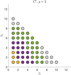
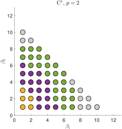
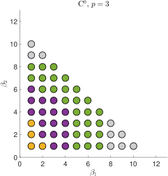
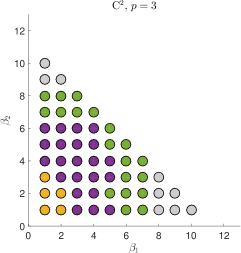
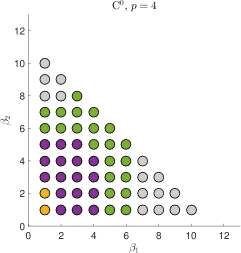
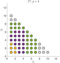
Figure 7: Optimal sets for the quarter-of-annulus problem with low-regular solution. From top to bottom row: $p=2,3,4$. Left column: $C^{0}$ B-spline basis; Right column: maximal continuity B-splines basis.

If we compute and look at the profits for this problem, we can indeed observe that the optimal sets are closer to a rectangle than a triangle, especially for $p=3,4$, i.e., the method of choice for this problem should be the standard (i.e., tensor-based) IGA, see Figure 7. It is also interesting to note that the profits decay more slowly along the second parametric direction (i.e., the angular direction in the physical domain), which therefore requires a finer discretization to be properly resolved, as one could have anticipated. The exact shape of the optimal set is however difficult to describe with a closed-form formula so that a dimension-adaptive scheme that iteratively chooses the best operator $\Delta_{\bm{\beta}}$ to be added to the sparse grid should be devised if one wants to take advantage of these partial sets, see e.g. [17].

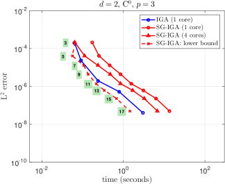
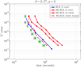
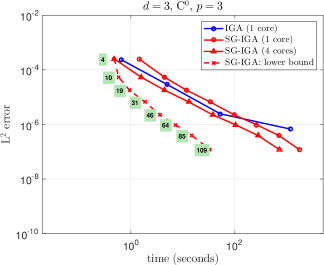
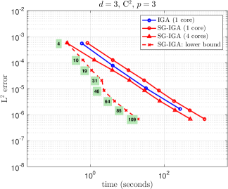
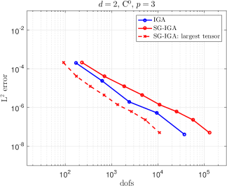
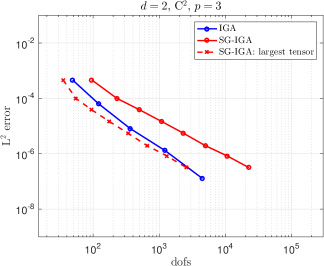
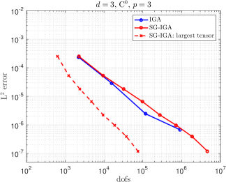
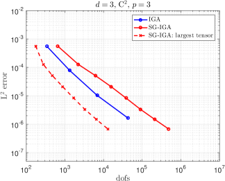
Figure 8: $L^{2}$ error vs. time for the quarter-of-annulus problem with low-regular solution. Here we fix $p=3$ and change $d$ (top row: $d=2$, bottom row: $d=3$) and the regularity of the B-splines basis (left column: $C^{0}$, right column: $C^{2}$). The dashed line is the lower bound that can be achieved if the number of available cores is at least equal to the number of components of the combination technique for each level, given by the numbers in green boxes.

Figure 9: $L^{2}$ error vs. dofs for the quarter-of-annulus problem with low-regular solution. Here we fix $p=3$ and change $d$ (top row: $d=2$, bottom row: $d=3$) and the regularity of the B-splines basis (left column: $C^{0}$, right column: $C^{2}$). In each figure, the dashed line represents the error of SG-IGA vs. the number of the degrees-of-freedom for the largest tensor grid in the combination technique.

Figures 9 and 9 show the decay of the error with respect to time and degrees-of-freedom, again focusing on the case $p=3$ only. These results confirm the underperformance of SG-IGA with respect to IGA in this case: compared to the problem with regular solution, cf. Figures 5 and 5, the rate of SG-IGA with respect to both time and degrees-of-freedom is now nearly identical to the rate of IGA and a larger number of cores is needed to obtain SG-IGA computational times close to IGA times (more than 4 cores in $d=2$, more than 1 core in $d=3$).

4.4 Radical meshes in the parametric domain

The solutions for the previous problem lack of (mixed) Sobolev regularity because of their singular behavior on the corners ($d=2$ and $d=3$) and edges ($d=3$) of the domain $\Omega$ (see [26]). This causes the slower convergence rate for both IGA and SG-IGA. To improve convergence in this situation, we adopt non-uniform radical meshes, see [22, 23]; see also [24, 25] for previous use of graded meshes in a sparse grids context. To this end, we compute the position of the $i$-th node on the $j$-th parametric dimension as $\xi_{i,j}=f(t_{i})$, where $t_{i}$ are knots of an equispaced grid over $[0,1]$ and $f$ is defined as follows, depending on a parameter $\gamma$:

$$f(t)=\begin{cases}\displaystyle\frac{t^{\gamma}}{1/2^{\gamma-1}}&\text{ if }t\leq\frac{1}{2},\\[8.0pt] \displaystyle 1-\frac{(1-t)^{\gamma}}{1/2^{\gamma-1}}&\text{ if }t>\frac{1}{2}.\end{cases}$$

Note that for $\gamma=1$ one recovers the equispaced mesh. We show some radical meshes for the $d=3$ version of the quarter-of-annulus domain in Figure 10.

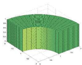
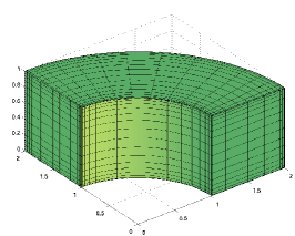
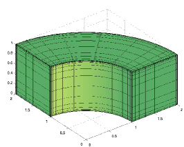
Figure 10: Knotlines of the quarter-of-annulus, $d=3$, for radical meshes with $\gamma=1,2,4$ (from left to right). Observe that the number of elements is identical in the three meshes.

In Figure 11 we show the value of the rate for the $H^{1}$ and $L^{2}$ error for IGA and SG-IGA applied to the two-dimensional version of the problem, for B-splines of order $p=2,3,4$, with minimal and maximal continuity, with radical meshes and $1\leq\gamma\leq 4.5$. As expected, the rate increases as $\gamma$ increases, until it reaches a maximum (then decreases in some cases). However, it is not easy to draw a general conclusion on the connection between the choice of $\gamma$, the degree $p$ and the regularity of the B-splines basis. Remarkably, for $p=2,3$ it seems that only B-splines with maximal regularity reach the optimal convergence rate. This is not the case for $p=4$. A possible explanation is that even for larger values of $\gamma$, the optimal set is not $\beta_{1}+\beta_{2}=constant$ but it becomes a more pronounced “convex shape” as $p$ increases, regardless of the continuity of the B-spline basis, see Figure 12. After inspection of Figure 11, we now repeat the analysis of error vs time and degrees-of-freedom setting $\gamma=3$.

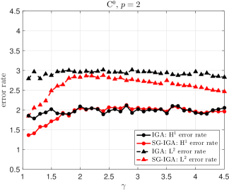
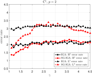
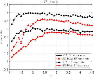
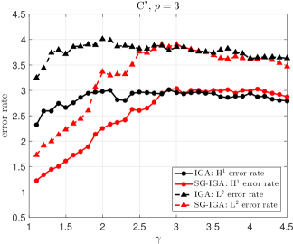
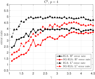
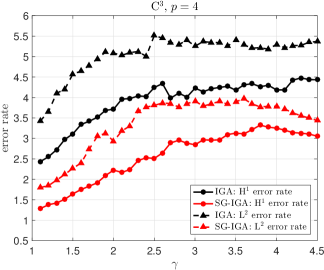
Figure 11: Measured convergence rate for increasing values of $\gamma$ for the quarter of annulus problem ($d=2$). From top to bottom: $p=2$ to $p=4$. The left column shows $C^{0}$ B-splines, the right column $C^{p-1}$ B-splines (maximal continuity).

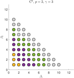
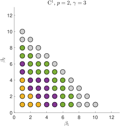
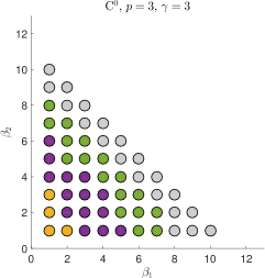
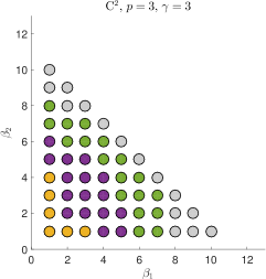
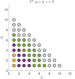
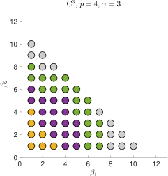
Figure 12: Optimal sets for the quarter-of-annulus problem with low-regular solution, for radical meshes with $\gamma=3$. From top to bottom row: $p=2,3,4$. Left column: $C^{0}$ B-spline basis; Right column: maximal continuity B-splines basis.

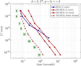
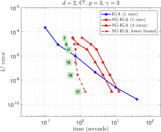
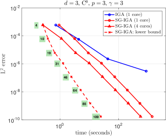
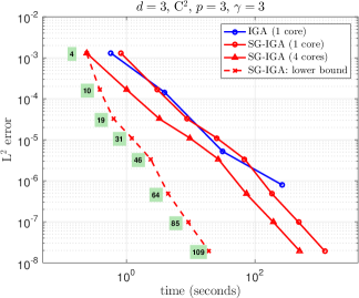
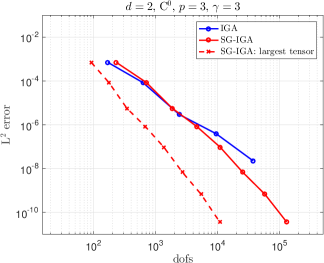
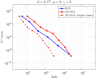
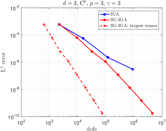
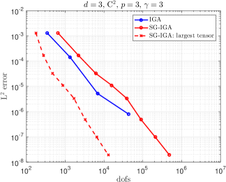
Figure 13: $L^{2}$ error vs. time for the quarter-of-annulus problem with low-regular solution, with radical meshes and $\gamma=3$. Here we fix $p=3$ and change $d$ (top row: $d=2$, bottom row: $d=3$) and the regularity of the B-splines basis (left column: $C^{0}$, right column: $C^{2}$). The dashed line is the lower bound that can be achieved if the number of available cores is at least equal to the number of components of the combination technique for each level, given by the numbers in green boxes.

Figure 14: $L^{2}$ error vs. dofs for the quarter-of-annulus problem with low-regular solution, with radical meshes and $\gamma=3$. Here we fix $p=3$ and change $d$ (top row: $d=2$, bottom row: $d=3$) and the regularity of the B-splines basis (left column: $C^{0}$, right column: $C^{2}$). In each figure, the dashed line represents the error of SG-IGA vs. the number of the degrees-of-freedom for the largest tensor grid in the combination technique.

The results obtained by introducing graded grids $\gamma=3$ are shown in Figures 14 and 14, and should be compared to the results for non-radical meshes reported in Figures 9 and 9. Inspecting the plots, it can be seen that SG-IGA is now competitive with IGA, especially for $d=3$, and indeed the results are now analogous to those reported in Figures 5 and 5 for the problem with regular solution.

4.5 Horseshoe domain

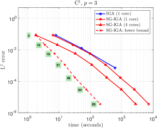
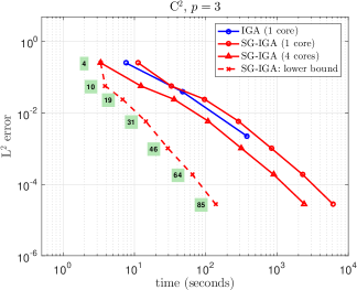
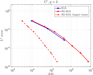
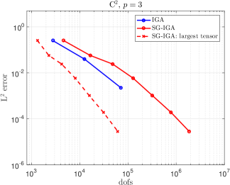
Figure 15: $L^{2}$ error vs. time (top row) and degrees-of-freedom (bottom row) for the horseshoe problem; the left column shows results with $C^{1}$ B-splines, while the right column with $C^{2}$ B-splines. For the bottom plots, the dashed line represents the error of SG-IGA vs. the number of the degrees-of-freedom for the largest tensor grid in the combination technique. Conversely, for the top plots the dashed line is the lower bound that can be achieved if the number of available cores is at least equal to the number of components of the combination technique for each level, given by the numbers in green boxes.

The last test we consider is on a more complex geometry, i.e., the horseshoe domain in Figure 2-right. Also in this case, we set $f(\mathbf{x})=1$, which will result in a solution with reduced regularity. Therefore, based on the previous experience, we tackle this problem with a graded mesh with $\gamma=3$. The results shown in Figure 15 for error versus time and degrees-of-freedom are similar to those for the three-dimensional version of quarter-of-annulus problem of Figure 14.

5 Conclusions

In this work we have shown how IGA solvers naturally fit in the sparse-grid construction framework, obtaining a method that on the one hand can improve the performances of standard full-tensor IGA approximations (if certain regularity requirements for the solution are met) and on the other hand extends the spectrum of applications of the sparse-grid technology to arbitrary domains and to basis functions with arbitrary order and regularity in a very convenient way. Moreover, the combination-technique version of the sparse-grid approximation allows to maximize the reuse of pre-existing IGA solver in a black-box fashion, and provides the user with a simple yet effective parallelization strategy for serial solvers. For problems whose solution does not feature the needed regularity for sparse grids to converge in a satisfactory way, a remedy consists in introducing properly tuned radical meshes in the parametric domain, even if more investigations are needed to explore the interplay between $\gamma$, $p$, and regularity of the basis.

This preliminary work opens to possible extensions and research directions. On the “methodological” level, it would be interesting to consider $p$ and $h-p$ sparsification for IGA solvers, as well as local adaptivity “à la sparse-grid”, see e.g. [17, 49, 50], which might be borrowed and interwined with the “classical” IGA refinement strategies such as [51, 52, 53]. Other interesting work directions are the sparsified version of IGA collocation solvers, and the combination of fast IGA implementations [7, 8] with the sparse-grid technology. Moreover, it might be worthwhile investigating sparse-adaptive solvers, in the spirit of what proposed while discussing Figures 6 and 7. Let us also remark that, even if the combination technique sometimes does not yield impressive gains over the regular full-tensor solver, it is nonetheless a fast way to build an approximation of the solution, and in this spirit it could be interesting to use it as a preconditioner for complex problems.

References

References

- [1] T. J. R. Hughes, J. A. Cottrell, Y. Bazilevs, Isogeometric analysis: CAD, finite elements, NURBS, exact geometry and mesh refinement, Computer Methods in Applied Mechanics and Engineering 194 (39) (2005) 4135–4195.
- [2] J. A. Cottrell, T. J. R. Hughes, Y. Bazilevs, Isogeometric Analysis: toward integration of CAD and FEA, John Wiley & Sons, 2009.
- [3] L. Beirao Da Veiga, A. Buffa, G. Sangalli, R. Vázquez, Mathematical analysis of variational isogeometric methods, Acta Numerica 23 (2014) 157–287.
- [4] L. Gao, Kronecker products on preconditioning, Ph.D. thesis, King Abdullah University of Science and Technology (2013).
- [5] L. Gao, V. M. Calo, Fast isogeometric solvers for explicit dynamics, Computer Methods in Applied Mechanics and Engineering 274 (2014) 19–41.
- [6] L. Gao, V. M. Calo, Preconditioners based on the alternating-direction-implicit algorithm for the 2d steady-state diffusion equation with orthotropic heterogeneous coefficients, Journal of Computational and Applied Mathematics 273 (2015) 274–295.
- [7] G. Sangalli, M. Tani, Isogeometric preconditioners based on fast solvers for the Sylvester equation, SIAM Journal on Scientific Computing 38 (6) (2016) A3644–A3671.
- [8] F. Calabrò, G. Sangalli, M. Tani, Fast formation of isogeometric galerkin matrices by weighted quadrature, Computer Methods in Applied Mechanics and Engineering.
- [9] A. Mantzaflaris, B. Jüttler, B. N. Khoromskij, U. Langer, Low rank tensor methods in galerkin-based isogeometric analysis, Computer Methods in Applied Mechanics and Engineering 316 (2017) 1062–1085.
- [10] P. Antolin, A. Buffa, F. Calabro, M. Martinelli, G. Sangalli, Efficient matrix computation for tensor-product isogeometric analysis: The use of sum factorization, Computer Methods in Applied Mechanics and Engineering 285 (2015) 817–828.
- [11] M. Donatelli, C. Garoni, C. Manni, S. Serra-Capizzano, H. Speleers, Symbol-based multigrid methods for Galerkin B-spline isogeometric analysis, SIAM Journal on Numerical Analysis 55 (1) (2017) 31–62.
- [12] C. Hofreither, S. Takacs, W. Zulehner, A robust multigrid method for isogeometric analysis in two dimensions using boundary correction, Computer Methods in Applied Mechanics and Engineering 316 (2017) 22 – 42, special Issue on Isogeometric Analysis: Progress and Challenges.
- [13] C. Zenger, Sparse grids, in: W. Hackbusch (Ed.), Parallel Algorithms for Partial Differential Equations, Vol. 31 of Notes on Numerical Fluid Mechanics, Vieweg, 1991, pp. 241–251.
- [14] H. Bungartz, Dünne gitter und deren anwendung bei der adaptiven lösung der dreidimensionalen poisson-gleichung, Ph.D. thesis, Institut für Informatik, Technische Universität Munchen (1992).
- [15] M. Griebel, A parallelizable and vectorizable multi-level-algorithm on sparse grids, in: W. Hackbusch (Ed.), Parallel Algorithms for Partial Differential Equations. Notes on Numerical Fluid Mechanics, Vol. 31, Verlag Vieweg, Braunschweig, 1991, pp. 94–100.
- [16] M. Griebel, M. Schneider, C. Zenger, A combination technique for the solution of sparse grid problems, in: P. de Groen, R. Beauwens (Eds.), Iterative Methods in Linear Algebra, IMACS, Elsevier, North Holland, 1992, pp. 263–281.
- [17] H. Bungartz, M. Griebel, Sparse grids, Acta Numer. 13 (2004) 147–269.
- [18] J. Garcke, Sparse grids in a nutshell, in: J. Garcke, M. Griebel (Eds.), Sparse Grids and Applications, Springer Berlin Heidelberg, Berlin, Heidelberg, 2013, pp. 57–80.
- [19] T. Dornseifer, C. Pflaum, Discretization of elliptic differential equations on curvilinear bounded domains with sparse grids, Computing 56 (3) (1996) 197–213.
- [20] H. J. Bungartz, T. Dornseifer, Sparse grids: Recent developments for elliptic partial differential equations, in: W. Hackbusch, G. Wittum (Eds.), Multigrid Methods V, Vol. 3 of Lecture Notes in Computational Science and Engineering, Springer, Berlin/Heidelberg, 1998.
- [21] S. Achatz, Higher order sparse grid methods for elliptic partial differential equations with variable coefficients, Computing 71 (1) (2003) 1–15.
- [22] I. Babuška, T. Strouboulis, The finite element method and its reliability, Numerical Mathematics and Scientific Computation, The Clarendon Press Oxford University Press, New York, 2001.
- [23] L. Beirão da Veiga, D. Cho, G. Sangalli, Anisotropic NURBS approximation in Isogeometric Analysis, Comput. Methods Appl. Mech. Engrg. 209-212 (2012) 1–11.
- [24] J. Garcke, M. Griebel, On the computation of the eigenproblems of hydrogen and helium in strong magnetic and electric fields with the sparse grid combination technique, Journal of Computational Physics 165 (2) (2000) 694 – 716.
- [25] M. Griebel, V. Thurner, The efficient solution of fluid dynamics problems by the combination technique, International Journal of Numerical Methods for Heat & Fluid Flow 5 (3) (1995) 251–269.
- [26] P. Grisvard, Elliptic problems in nonsmooth domains, Vol. 24 of Monographs and Studies in Mathematics, Pitman (Advanced Publishing Program), Boston, MA, 1985.
- [27] L. Beiraõ da Veiga, A. Buffa, G. Sangalli, R. Vázquez, Mathematical analysis of variational isogeometric methods, Acta Numerica 23 (2014) 157–287.
- [28] C. de Boor, A practical guide to splines, revised Edition, Vol. 27 of Applied Mathematical Sciences, Springer-Verlag, New York, 2001.
- [29] G. Wasilkowski, H. Wozniakowski, Explicit cost bounds of algorithms for multivariate tensor product problems, Journal of Complexity 11 (1) (1995) 1 – 56.
- [30] H.-J. Bungartz, M. Griebel, D. Röschke, C. Zenger, Pointwise convergence of the combination technique for the Laplace equation, East-West J. Numer. Math. 2 (1994) 21–45.
- [31] M. Hegland, J. Garcke, V. Challis, The combination technique and some generalisations, Linear Algebra and its Applications 420 (2–3) (2007) 249 – 275.
- [32] M. Griebel, H. Harbrecht, On the convergence of the combination technique, in: J. Garcke, D. Pflüger (Eds.), Sparse Grids and Applications - Munich 2012, Vol. 97 of Lecture Notes in Computational Science and Engineering, Springer International Publishing, 2014, pp. 55–74.
- [33] C. Reisinger, Analysis of linear difference schemes in the sparse grid combination technique, IMA Journal of Numerical Analysis 33 (2) (2013) 544–581.
- [34] C. Reisinger, G. Wittum, Efficient hierarchical approximation of high-dimensional option pricing problems, SIAM Journal on Scientific Computing 29 (1) (2007) 440–458.
- [35] M. Griebel, H. Harbrecht, On the construction of sparse tensor product spaces, Mathematics of Computation 82 (282) (2013) 975–994.
- [36] M. Griebel, H. Harbrecht, A note on the construction of L-fold sparse tensor product spaces, Constructive Approximation 38 (2) (2013) 235–251.
- [37] C. Pflaum, A. Zhou, Error analysis of the combination technique, Numerische Mathematik 84 (2) (1999) 327–350.
- [38] H.-J. Bungartz, M. Griebel, D. Röschke, C. Zenger, Two proofs of convergence for the combination technique for the efficient solution of sparse grid problems, in: In Domain decomposition methods in scientific and engineering computing (University Park, PA), 1993.
- [39] R. Vázquez, A new design for the implementation of isogeometric analysis in Octave and Matlab: GeoPDEs 3.0, Computer & Mathematics with Applications 72 (3) (2016) 523–554.
- [40] G. Sangalli, M. Tani, Matrix-free isogeometric analysis: the computationally efficient -method, arXiv preprint arXiv:1712.08565.
- [41] M. Griebel, The combination technique for the sparse grid solution of PDEs on multiprocessor machine, Parallel Processing Letters 2 (1992) 61–70.
- [42] M. Heene, D. Pflüger, Efficient and scalable distributed-memory hierarchization algorithms for the sparse grid combination technique, in: Parallel Computing: On the Road to Exascale, Vol. 27 of Advances in Parallel Computing, IOS Press, 2016, pp. 339–348.
- [43] M. Heene, D. Pflüger, Scalable algorithms for the solution of higher-dimensional PDEs, in: H.-J. Bungartz, P. Neumann, W. E. Nagel (Eds.), Software for Exascale Computing - SPPEXA 2013-2015, Springer International Publishing, Cham, 2016, pp. 165–186.
- [44] J. Garcke, M. Hegland, O. Nielsen, Parallelisation of sparse grids for large scale data analysis, The ANZIAM Journal 48 (1) (2006) 11–22.
- [45] S. Martello, P. Toth, Knapsack problems: algorithms and computer implementations, Wiley-Interscience series in discrete mathematics and optimization, J. Wiley & Sons, 1990.
- [46] M. Griebel, S. Knapek, Optimized general sparse grid approximation spaces for operator equations, Math. Comp. 78 (268) (2009) 2223–2257.
- [47] F. Nobile, L. Tamellini, R. Tempone, Convergence of quasi-optimal sparse-grid approximation of Hilbert-space-valued functions: application to random elliptic PDEs, Numerische Mathematik 134 (2) (2016) 343–388.
- [48] M. Dauge, Elliptic Boundary Value Problems on Corner Domains: Smoothness and Asymptotics of Solutions, Lecture Notes in Mathematics, Springer Berlin Heidelberg, 2006.
- [49] J. Jakeman, R. Archibald, D. Xiu, Characterization of discontinuities in high-dimensional stochastic problems on adaptive sparse grids, J. Comput. Phys. 230 (10).
- [50] D. Pflüger, Spatially adaptive refinement, in: J. Garcke, M. Griebel (Eds.), Sparse Grids and Applications, Springer Berlin Heidelberg, Berlin, Heidelberg, 2013, pp. 243–262.
- [51] C. Giannelli, B. Jüttler, H. Speleers, THB-splines: The truncated basis for hierarchical splines, Comput. Aided Geom. Design. 29 (7) (2012) 485 – 498.
- [52] T. Dokken, T. Lyche, K. F. Pettersen, Polynomial splines over locally refined box-partitions, Comput. Aided Geom. Design 30 (3) (2013) 331–356.
- [53] C. Giannelli, B. Jüttler, H. Speleers, Strongly stable bases for adaptively refined multilevel spline spaces, Adv. Comput. Math. (2013) 1–32.