Extreme Quantum Advantage for Rare-Event Sampling

Abstract

We introduce a quantum algorithm for efficient biased sampling of the rare events generated by classical memoryful stochastic processes. We show that this quantum algorithm gives an extreme advantage over known classical biased sampling algorithms in terms of the memory resources required. The quantum memory advantage ranges from polynomial to exponential and when sampling the rare equilibrium configurations of spin systems the quantum advantage diverges.

I Introduction

From earthquakes to financial market crashes, rare events are associated with catastrophe—from decimated social infrastructure and the substantial loss of life to global economic collapse. Though rare, their impact cannot be ignored. Prediction and modeling such rare events is essential to mitigating their effects. However, this is particularly challenging, often requiring huge datasets and massive computational resources, precisely because the events of interest are rare.

Ameliorating much of the challenge, biased or extended sampling [1, 2] is an effective and now widely-used method for efficient generation and analysis of rare events. The underlying idea is simple to state: transform a given distribution to a new one where previously rare events are now typical. This concept was originally proposed in 1961 by Miller to probe the rare events generated by discrete-time, discrete-value Markov stochastic processes [3]. It has since been extended to address non-Markovian processes [4]. The approach was also eventually adapted to continuous-time first-order Markov processes [5, 6, 7]. Today, the statistical analysis of rare events is a highly developed toolkit with broad applications in sciences and engineering [8]. Given this, it is perhaps not surprising that the idea and its related methods appear under different appellations, depending on the research arena. For example, large deviation theory refers to the s-ensemble method [9, 10], the exponential tilting algorithm [11, 12], or as generating twisted distributions.

In 1997, building on biased sampling, Torrie and Valleau introduced umbrella sampling into Monte Carlo simulation of systems whose energy landscapes have high energy barriers and so suffer particularly from poor sampling [13]. Since then, stimulated by computational problems arising in statistical mechanics, the approach was generalized to Ferrenberg-Swendsen reweighting, later still to weighted histogram analysis [14], and more recently to Wang-Landau sampling [15].

When generating samples for a given stochastic process one can employ alternative types of algorithm. There are two main types—Monte Carlo or finite-state machine algorithms. Here, we consider finite-state machine algorithms based on Markov chains (MC) [16, 17] and hidden Markov models (HMM) [18, 19, 20]. For example, if the process is Markovian one uses MC generators and, in more general cases, one uses HMM generators.

When evaluating alternative approaches the key questions that arise concern algorithm speed and memory efficiency. For example, it turns out there are HMMs that are always equally or more memory efficient than MCs. There are many finite-state HMMs for which the analogous MC is infinite-state [21]. And so, when comparing all HMMs that generate the same process, one is often interested in those that are most memory efficient. For a generic stochastic process, the most memory efficient classical HMM known currently is the $\epsilon$-machine of computational mechanics [22]. The memory it requires is called the process’ statistical complexity $C_{\mu}$ [23].

Today, we have come to appreciate that several important mathematical problems can be solved more efficiently using a quantum computer. Examples include quantum algorithms for integer factorization [24], search [25], eigen-decomposition [26], and solving linear systems [27]. Not long ago and for the first time, Ref. [28] provided a quantum algorithm that can perform stochastic process sample-generation using less memory than the best-known classical algorithms. Recently, using a stochastic process’ higher-order correlations, a new quantum algorithm—the q-machine—substantially improved this efficiency and extended its applicability [29]. More detailed analysis and a derivation of the closed-form quantum advantage of the q-machine is given in a sequel [30]. Notably, the quantum advantage has been verified experimentally for a simple case [31].

The following brings together techniques from large deviation theory, classical algorithms for stochastic process generation, computational complexity theory, and the newly introduced quantum algorithm for stochastic process generation to propose a new, memory efficient quantum algorithm for the biased sampling problem. We show that there can be an extreme advantage in the quantum algorithm’s required memory compared to the best known classical algorithm. Two examples are analyzed here. The first is the simple, but now well-studied perturbed coin process. The second is a more physical example—a stochastic process that arises from the Ising next-nearest-neighbor spin system in contact with thermal reservoir.

II Classical Algorithm

The object for which we wish to generate samples is a discrete-time, discrete-value stochastic process [32, 18]: a probability space $\mathcal{P}=\big{\{}\mathcal{A}^{\infty},\Sigma,\mathbb{P}(\cdot)\big{\}}$, where $\mathbb{P}(\cdot)$ is a probability measure over the bi-infinite chain $\ldots{X}_{-2}{X}_{-1}{X}_{0}{X}_{1}{X}_{2}\ldots$, each random variable ${X}_{i}$ takes values in a finite, discrete alphabet $\mathcal{A}$, and $\Sigma$ is the $\sigma$-algebra generated by the cylinder sets in $\mathcal{A}^{\infty}$. For simplicity we consider only ergodic stationary processes: that is, $\mathbb{P}(\cdot)$ is invariant under time translation—$\mathbb{P}({X}_{i_{1}}{X}_{i_{2}}\cdots{X}_{i_{m}})=\mathbb{P}({X}_{i_{1}+n}{X}_{i_{2}+n}\cdots{X}_{i_{m}+n})$ for all $n$, $m$—and over successive realizations.

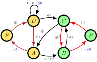
Figure 1: Hidden Markov model generator of a stochastic process with infinite-range statistical dependencies that requires an HMM with only six states. To generate the same process via a Markov chain requires one with an infinite number of states and so infinite memory.

Sampling or generating a given stochastic process refers to producing a finite realization that comes from the process’ probability distribution. Generally, generating a process via its probability measure $\mathbb{P}(\cdot)$ is impossible due to the vast number of allowed realizations and, as a result, this prosaic approach requires an unbounded amount of memory. Fortunately, there are more compact ways than specifying in-full the probability measure on the sequence sigma algebra. This recalls the earlier remark that HMMs can be arbitrarily more compact than alternative algorithms for the task of generation.

An HMM is specified by a tuple $\big{\{}\bm{\mathcal{S}},\mathcal{A},\{T^{({x})},{x}\in\mathcal{A}\}\big{\}}$. In this, $\bm{\mathcal{S}}$ is a finite set of states, $\mathcal{A}$ is a finite alphabet, and $\{T^{({x})},{x}\in\mathcal{A}\}$ is a set of $|\bm{\mathcal{S}}|\times|\bm{\mathcal{S}}|$ substochastic symbol-labeled transition matrices whose sum $T=\sum_{{x}\in\mathcal{A}}T^{({x})}$ is a stochastic matrix.

As an example, consider the HMM state-transition diagram shown in Fig. 1, where $\bm{\mathcal{S}}=\{A,B,C,D,E,F\}$, $\mathcal{A}=\{0,1,2\}$, and we have three $6\times 6$ substochastic matrices $T^{(0)}$, $T^{(1)}$, and $T^{(2)}$. Each edge is labeled $p|{\color[rgb]{0,0,1}x}$ denoting the transition probability $p$ and a symbol ${\color[rgb]{0,0,1}x}\in\mathcal{A}$ which is emitted during the transition. In this HMM, of the two edges exiting state $C$, one enters state $B$ and the other enters state $A$. The edges from $C$ to $A$ and $C$ to $B$ are labeled by $\frac{1}{2}|{\color[rgb]{0,0,1}1}$ and $\frac{1}{2}|{\color[rgb]{0,0,1}0}$. This simply means that if the HMM is in the state $C$, then with probability $\frac{1}{2}$ it goes to the state $A$ and emits the symbol $\color[rgb]{0,0,1}1$ and with probability $\frac{1}{2}$ it goes to state $B$ and emits symbol $\color[rgb]{0,0,1}0$. Following these transition rules in succession generates realizations in the HMM’s process.

How does this generation method compare to generating realizations of the same process via a finite Markov chain. It turns out that this cannot be implemented, since generating a symbol can depend on the infinite history. That is, the process has infinite Markov order. As a result, to generate a realization using a Markov chain one needs an infinite number of Markovian states. In other words, implementing the Markov chain algorithm to generate process samples on a conventional computer requires an infinite amount of memory.

To appreciate the reason behind the process’ infinite Markov order, refer to Fig. 1’s HMM. There are two length-$3$ state-loops consisting of the edges colored red (right side of state-transition diagram) and those colored maroon (left side). Note that if the HMM generates $n$ $\color[rgb]{0,0,1}1$s in a row, we will not know the HMM’s current state, only that it is either $A$, $D$, or $E$. This state uncertainty (entropy) is bounded away from $0$. The observation holds for the other loop and its sequences of symbol $\color[rgb]{0,0,1}0$ and the consequent ambiguity among states $B$, $C$, and $F$. Thus, there exist process realizations from which we cannot determine the future statistics, independent of the number of symbols seen. This means that the process statistics depend on infinite past sequences—the process has infinite Markov order. To emphasize, implementing a MC algorithm for this requires infinite memory. The contrast with the finite HMM method is an important lesson: HMMs are strictly more powerful generators, as a class of algorithms, than Markov chain generators.

For any given process $\mathcal{P}$, there are an infinite number of HMMs that generate it. Therefore, one is compelled to ask, Which algorithm requires the least memory for implementation? The best known implementation, and provably the optimal predictor, is known as the $\epsilon$-machine [33, 22]. The states of the $\epsilon$-machine are called causal states; we denote this set $\bm{\mathcal{S}}$.

The average memory required for $M(\mathcal{P})$ to generate process $\mathcal{P}$ is given by the process’ statistical complexity $C_{\mu}(\mathcal{P})$ [23]. To calculate it:

1. Compute the stationary distribution $\pi$ over causal states. $\pi$ is the left eigenvector of the state-transition matrix $T$ with eigenvalue $1$: $\pi T=\pi$.

2. Calculate the state’s Shannon entropy $\operatorname{H}[\bm{\mathcal{S}}]=-\sum_{\sigma\in\bm{\mathcal{S}}}\pi(\sigma)\log_{2}\pi(\sigma)$.

Thus, $C_{\mu}=\operatorname{H}[\bm{\mathcal{S}}]$ measures the (ensemble average) memory required to generate the process.

Another important, companion measure is $h_{\mu}$, the process’ metric entropy (or Shannon entropy rate) [34]:

$$h_{\mu}(\mathcal{P})=-\lim_{n\to\infty}\frac{1}{n}\sum_{w\in\mathcal{A}^{n}}\mathbb{P}(w)\log_{2}\mathbb{P}(w)~{}.$$

Although sometimes confused, it is important to emphasize that $h_{\mu}$ describes randomness in the realizations, while $C_{\mu}$ describes the required memory for process generation.

III Quantum memory advantage

Recently, it was shown that a quantum algorithm for process generation can use less memory than the best known classical algorithm ($\epsilon$-machine) [28]. We refer to the ratio of required classical memory $C_{\mu}$ to quantum memory as the quantum advantage. Taking into account a process’ higher-order correlations, a new quantum algorithm—the q-machine—was introduced that substantially improves the original quantum algorithm and is, to date, the most memory-efficient quantum algorithm known for process generation [29]. Closed-form expressions for the quantum advantage are given in [30].

Importantly, the quantum advantage was recently verified experimentally for the simple perturbed coins process [31]. It has been found that the q-machine sometimes confers an extreme quantum-memory advantage. For example, for generation of ground-state configurations (in a Dyson-type spin model with $N$-nearest-neighbor interactions at temperature $T$), the quantum advantage scales as $NT^{2}/\log_{2}{T}$ [35, 36].

One consequence of this quantum advantage arises in model selection [37]. Statistical inference of models for stochastic systems often involves controlling for model size or memory. The following applies this quantum advantage to find gains in the setting of biased sampling of a process’ rare events. In particular, we will develop tools to determine how the memory requirements of classical and quantum algorithms vary over rare-event classes.

IV Quantum algorithm

We define the quantum machine of a stochastic process $\mathcal{P}$, by $QM(\mathcal{P})=\{\mathcal{H},\mathcal{A},\{K_{{x}},{x}\in\mathcal{A}\}\}$, where $\mathcal{H}$ denotes the Hilbert space in which quantum states reside, $\mathcal{A}$ is the same alphabet as the given process’, and $\{K_{{x}},{x}\in\mathcal{A}\}$ is a set of Kraus operators we use to specify the measurement protocol for states [38]. Assume we have the state (or density matrix) $\rho_{0}\in\mathcal{B}(H)$ in hand. We perform a measurement and, as a result, we measure $X$. The probability of yielding symbol $x_{0}\in X$ is:

$$\mathbb{P}(X=x_{0}|\rho_{0})=\mathrm{tr}\left(K_{x_{0}}\rho_{0}K_{x_{0}}^{\dagger}\right)~{}.$$

After measurement with outcome $X=s_{0}$, the new quantum state is:

$$\rho_{1}=\frac{K_{x_{0}}\rho_{0}K_{x_{0}}^{\dagger}}{\mathrm{tr}(K_{x_{0}}\rho_{0}K_{x_{0}}^{\dagger})}~{}.$$

Repeating these measurements generates a stochastic process. The process potentially could be nonergodic, depending on the initial state $\rho_{0}$. Starting the machine in the stationary state defined by:

$$\rho_{s}=\sum\limits_{x\in\mathcal{A}}K_{x}\rho_{s}K_{x}^{\dagger}~{},$$

and doing a measurements over and over again leads to generating a stationary stochastic process over ${x}\in\mathcal{A}$. For any given process, $\rho_{s}$ can be calculated by the method introduced in Ref. [30].

Our immediate goal is to design a quantum generator of a given classical process. (Section VI will then take the given process to represent a rare-event class of some other process.) For now, we start with the process’ $\epsilon$-machine. The construction consists of three steps, as follows.

First: Map every causal state $\sigma_{i}\in\bm{\mathcal{S}}$ to a pure quantum state $\ket{\eta_{i}}$. Each signal state $\ket{\eta_{i}}$ encodes the set of length-$R$ sequences that may follow $\sigma_{i}$, as well as each corresponding conditional probability:

$$\ket{\eta_{i}}\equiv\sum\limits_{w\in\mathcal{A}^{R}}\sum\limits_{\sigma_{j}\in\bm{\mathcal{S}}}{\sqrt{\mathbb{P}(w|\sigma_{i})}~{}\ket{w}}~{},$$

where $w$ denotes a length-$R$ sequence, $\mathbb{P}(w|\sigma_{i})=\mathbb{P}(X_{0}\cdots X_{R-1}=w|\mathcal{S}_{0}=\sigma_{i})$, and $R$ is the process’ the Markov order. The resulting Hilbert space is $\mathcal{H}_{w}$ with size $|\mathcal{A}|^{R}$, the number of length-$R$ sequences, with basis elements $\ket{w}=\ket{x_{0}}\otimes\cdots\otimes\ket{x_{R-1}}$.

Second: Form a matrix $\Xi$ by assembling the signal states:

$$\Xi=\begin{bmatrix}\ket{\eta_{0}}&&\ket{\eta_{1}}&&\cdots&&\ket{\eta_{|\bm{\mathcal{S}}|-1}}\end{bmatrix}~{}.$$

From here on out, we assume all the $\ket{\eta_{i}}$s are linearly independent. (This holds for general processes except for some special cases, which we discuss elsewhere.) Define $|\bm{\mathcal{S}}|$ new bra states $\ket{\widetilde{\eta_{i}}}$:

$$\begin{bmatrix}\bra{\widetilde{\eta_{0}}}\\ \bra{\widetilde{\eta_{1}}}\\ \cdots\\ \bra{\widetilde{\eta_{|\bm{\mathcal{S}}|-1}}}\end{bmatrix}=\Xi^{-1}~{}.$$

That is, we design the new bra states such that we obtain the identity:

$$\begin{bmatrix}\bra{\widetilde{\eta_{0}}}\\ \bra{\widetilde{\eta_{1}}}\\ \cdots\\ \bra{\widetilde{\eta_{|\bm{\mathcal{S}}|-1}}}\end{bmatrix}\begin{bmatrix}\ket{\eta_{0}}&&\ket{\eta_{1}}&&\cdots&&\ket{\eta_{|\bm{\mathcal{S}}|-1}}\end{bmatrix}=\mathrm{I}~{}.$$

Third: Define $|\mathcal{A}|$ Kraus operators $K_{i}$s via:

$$K_{x}=\sum_{i,j}\sqrt{T_{ij}^{x}}\ket{\eta_{j}}\bra{\widetilde{\eta_{i}}}~{}.$$

Using the quantum generator $QM(\mathcal{P})$, the required average memory for generating process $\mathcal{P}$ is $C_{q}(\mathcal{P})=S(\rho_{s})$, where $S(\rho)=-\mathrm{tr}(\rho\log\rho)$ denotes the von Neumann entropy [38]. References [29, 35] explain why $C_{q}$ is the quantum machine’s required memory.

V Typical Realizations

At this point, we established classical and quantum representations of processes and characterized their respective memory requirements. Our purpose now turns to this set-up to monitor the classical and quantum resources required to generate probability classes of a process’ realizations.

The concept of a stochastic process is quite general. Any physical system that exhibits stochastic dynamics in time or space may be thought of as generating a stochastic process. In the spatial setting one considers not time evolution, but rather the spatial “dynamic”. For example, consider a one-dimensional noninteracting Ising spin-½ chain with classical Hamiltonian $H=-\sum_{i=1}^{n}h\sigma_{i}$ in contact with a thermal reservoir at temperature $T$. After thermalizing, a spin configuration at one instant of time may be thought of as having been generated left-to-right (or equivalently right-to-left). The probability distribution over these spatial-translation invariant configurations defines a stationary stochastic process—a simple Markov random field.

For $n\gg 1$, one can ask for the probability of seeing $k$ up spins. The Strong Law of Large Numbers [39] guarantees that for large $n$, the ratio $k/n$ almost surely converges to $p_{\uparrow}=\tfrac{1}{2}\left(1+\tanh(h/k_{\textrm{B}}T)\right)$. That is:

$$\mathbb{P}\left(\lim_{n\to\infty}\frac{k}{n}=p_{\uparrow}\right)=1~{}.$$

Informally, a typical sequence is one that has close to $p_{\uparrow}n$ spin ups. However, this does not preclude seeing other kinds of rare long runs, e.g., all up-spins or all down-spin. It simply means that the latter are rare events.

Now let us formally define the concept of typical realizations and, consequently, rare ones. Consider a given process $\mathcal{P}$ and let $\mathcal{A}^{n}$ denote its set of length-$n$ realizations. Then, for an arbitrary $0<\epsilon\ll 1$ the process’ typical set [40, 41, 42] is defined:

$$A_{\epsilon}^{n}\!\equiv\!\{w:2^{-n(h_{\mu}+\epsilon)}\leq\mathbb{P}(w)\leq 2^{-n(h_{\mu}-\epsilon)},w\in\mathcal{A}^{n}\},$$ (1)

where $h_{\mu}$ is the process’ Shannon entropy rate, introduced above.

According to the Shannon-McMillan-Breiman theorem [43, 44, 45], for a given $\epsilon\ll 1$ and sufficiently large $n^{*}$:

$$\mathbb{P}(w\notin A_{\epsilon}^{n},w\in\mathcal{A}^{n})\leq\epsilon,\forall n\geq n^{*}~{}.$$ (2)

There are two important lessons here. First, from Eq. (1) we see that all sequences in the typical set have approximately the same probability. More precisely, the probability of typical sequences decays at the same exponential rate. The following adapts this to use decay rates to identify distinct sets of rare events. Second, coming from Eq. (2), for large $n$ the probability of sequences falling outside the typical set is close to zero—these are the sets of rare sequences.

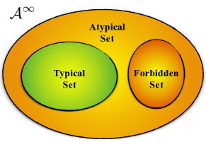
Figure 2: For a given process, the space $\mathcal{A}^{\infty}$ of all sequences is partitioned into those that are forbidden by the process, sequences in the typical set, and sequences not forbidden nor typical—the atypical or rare sequences.

Another important consequence of the theorem is that sequences generated by a stationary ergodic process fall into one of three partitions; see Fig. 2. The first contains those that are never generated; they fall in the the forbidden set. For example, the HMM in Fig. 1 never generates sequences that have consecutive $2$s. The second partition consists of those in the typical set—the set with probability close to one, as in Eq. (1). And, the last contains sequences in a family of atypical sets—realizations that are rare to different degrees. We now refine this classification by dividing the atypical set into identifiable subsets, each with their own characteristic rarity.

Mirroring the familiar Boltzmann weight in statistical physics [46], in the $n\to\infty$ limit, we define the subsets $\Lambda^{\mathcal{P}}_{U}\subset\mathcal{A}^{\infty}$ for a process $\mathcal{P}$ as:

$$\Lambda^{\mathcal{P}}_{U,n} =\left\{w:-\frac{\log_{2}\mathbb{P}(w)}{n}=U,\ w\in\mathcal{A}^{n}\right\}$$ (3)

$$\Lambda^{\mathcal{P}}_{U} =\lim_{n\to\infty}\Lambda^{\mathcal{P}}_{U,n}~{}.$$

This partitions $\mathcal{A}^{\infty}$ into disjoint subsets $\Lambda^{\mathcal{P}}_{U}$ in which all $w\in\Lambda^{\mathcal{P}}_{U}$ have the same probability decay rate $U$. Physics vernacular would speak of the sequences having the same energy density $U$. Figure 3 depicts these subsets as “bubbles” of equal energy. Equation (1) says the typical set is that bubble with energy equal to the process’ Shannon entropy rate: $U=h_{\mu}$. All the other bubbles contain rare events, some rarer than others. They exhibit faster or slower probability decay rates.

Employing a process’ HMM to generate realizations produces sequences in the typical set with probability close to one and, rarely, atypical sequences. Imagine that one is interested in a particular class of rare sequences, say, those with energy $U$ ($\Lambda^{\mathcal{P}}_{U}$). (One might be concerned about the class of large-magnitude earthquakes or the emergence of major instabilities in the financial markets, for example.) How can one efficiently generate these rare sequences? We now show that there is a new process $\mathcal{P}^{U}$ whose typical set is $\Lambda^{\mathcal{P}}_{U}$ and this returns us directly to the challenge of biased sampling.

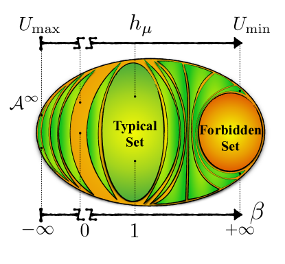
Figure 3: The space of all sequences $\mathcal{A}^{\infty}$ partitioned into $\Lambda_{U}$s—isoenergy or equal probability-decay-rate bubbles—in which all sequences in the same $\Lambda_{U}$ have the same energy $U$. The typical set is one such bubble with energy equal to Shannon entropy rate: $U=h_{\mu}$. Another important class is the forbidden set, in which all sequences do not occur. The forbidden set can also be interpreted as the subset of sequences with infinite positive energy. By applying the map $\mathcal{B}_{\beta}$ to the process and changing $\beta$ continuously from $-\infty$ to $+\infty$ (excluding $\beta=0$) one can generate any rare class of interest $\Lambda^{\mathcal{P}}_{U}$. $\beta\to-\infty$ corresponds to the most probable sequences with the largest energy density $U_{\text{max}}$, $\beta=1$ corresponds to the typical set and $\beta\to+\infty$ corresponds to the least probable sequences with the smallest energy density $U_{\text{min}}$.

VI Biased Sampling

Consider a finite set of configurations $\{c_{i}\}$ with probabilities specified by distribution $\mathbb{P}(\cdot)$ and an associated set $\{\omega_{i}\}$ of weighting factors. Consider the procedure of reweighting that introduces a new distribution $\widetilde{\mathbb{P}}(\cdot)$ over configurations where:

$$\widetilde{\mathbb{P}}(c_{i})=\frac{\mathbb{P}(c_{i})\exp(\omega_{i})}{\sum\limits_{i}\mathbb{P}(c_{i})\exp(\omega_{i})}~{}.$$

Given a process $\mathcal{P}$ and its $\epsilon$-machine $M(\mathcal{P})$, How do we construct an $\epsilon$-machine $M(\mathcal{P}^{U})$ that generates $\mathcal{P}$’s atypical sequences at some energy density $U\neq h_{\mu}$ or, as we denoted it, the set $\Lambda^{\mathcal{P}}_{U}$? Here, we answer this question by constructing a map $\mathcal{B}_{\beta}:\mathcal{P}\rightarrow\mathcal{P}_{\beta}$ from the original process $\mathcal{P}$ to a new one $\mathcal{P}_{\beta}$. The map is parametrized by $\beta\in\mathbb{R}/\{0\}$ which indexes the rare set of interest. (We use $\beta$ for convenience here, but it is related to $U$ by a function introduced shortly.) Both processes $\mathcal{P}=\big{\{}\mathcal{A}^{\infty},\Sigma,\mathbb{P}(\cdot)\big{\}}$ and $\mathcal{P}_{\beta}=\big{\{}\mathcal{A}^{\infty},\Sigma,\mathbb{P}_{\beta}(\cdot)\big{\}}$ are defined on the same measurable sequence space. The measures differ, but their supports (allowed sequences) are the same. For simplicity we refer to $\mathcal{B}_{\beta}$ as the $\beta$-map.

Assume we are given $M(\mathcal{P})=\big{\{}\bm{\mathcal{S}},\mathcal{A},\{T^{({x})},{x}\in\mathcal{A}\}\big{\}}$. We showed that for every probability decay rate or energy density $U$, there exists a particular $\beta$ such that $M(\mathcal{P}_{\beta})$ typically generates the words in $\Lambda^{\mathcal{P}}_{U,n}$ for large $n$ [48]. The $\beta$-map which establishes this is calculated by a construction that relates $M(\mathcal{P})$ to $M(\mathcal{P}_{\beta})=\big{\{}\bm{\mathcal{S}},\mathcal{A},\{\mathbf{S}_{\beta}^{({x})},{x}\in\mathcal{A}\}\big{\}}$—the HMM that generates $\mathcal{P}_{\beta}$:

1. For each ${x}\in\mathcal{A}$, construct a new matrix $\mathbf{T}^{({x})}_{\beta}$ for which $\big{(}\mathbf{T}^{({x})}_{\beta}\big{)}_{ij}=\big{(}\mathbf{T}^{({x})}\big{)}_{ij}^{\beta}$.

2. Form the matrix $\mathbf{T}_{\beta}=\sum_{{x}\in\mathcal{A}}T^{({x})}_{\beta}$.

3. Calculate $\mathbf{T}_{\beta}$’s maximum eigenvalue ${\widehat{\lambda}_{\beta}}$ and corresponding right eigenvector ${\widehat{\mathbf{r}}_{\beta}}$.

4. For each ${x}\in\mathcal{A}$, construct new matrices $\mathbf{S}_{\beta}^{({x})}$ for which:

   $$\big{(}{\textbf{S}}^{({x})}_{\beta}\big{)}_{ij}=\frac{\big{(}\mathbf{T}^{({x})}_{\beta}\big{)}_{ij}({\widehat{\mathbf{r}}_{\beta}})_{j}}{{\widehat{\lambda}_{\beta}}({\widehat{\mathbf{r}}_{\beta}})_{i}}~{}.$$

Having constructed the new process $\mathcal{P}_{\beta}$ by introducing its generator, we use the latter to produce some rare set of interest $\Lambda^{\mathcal{P}}_{U,n}$.

Theorem 1.

In the limit $n\to\infty$, within the new process $\mathcal{P}_{\beta}$ the probability of generating realizations from the set $\Lambda^{\mathcal{P}}_{U,n}$ converges to one:

$$\lim_{n\to\infty}\mathbb{P}_{\beta}(\Lambda^{\mathcal{P}}_{U,n})=1~{},$$

where:

$$U=\beta^{-1}\big{(}h_{\mu}(\mathcal{P}_{\beta})-\log_{2}{\widehat{\lambda}_{\beta}}\big{)}~{}.$$ (4)

In addition, in the same limit the process $\mathcal{P}_{\beta}$ assigns equal energy densities over all the members of the set $\Lambda^{\mathcal{P}}_{U,n}$.

Proof.

See Ref. [48].

As a result, for large $n$ the process $\mathcal{P}_{\beta}$ typically generates the set $\Lambda^{\mathcal{P}}_{U,n}$ with the specified energy $U$. The process $\mathcal{P}_{\beta}$ is sometimes called the auxiliary, driven, or effective process [49, 50, 51]. Examining the form of the energy, one sees that there is a one-to-one relationship between $\beta$ and $U$. And so, we can equivalently denote the process $\mathcal{P}_{\beta}$ by $\mathcal{P}^{U}$. More formally, every word in $\Lambda^{\mathcal{P}}_{U}$ with probability measure one is in the typical set of process $\mathcal{P}_{\beta}$.

The $\beta$-map construction guarantees that the HMMs $M(\mathcal{P})$ and $M(\mathcal{P}_{\beta})$ have the same states and transition topology: $\big{(}\mathbf{T}^{({x})}_{\beta}\big{)}_{ij}\neq 0\iff\big{(}{\textbf{S}}^{({x})}_{\beta}\big{)}_{ij}\neq 0$. The only difference is in their transition probabilities. $M(\mathcal{P}_{\beta})$ is not necessarily an $\epsilon$-machine—the most memory-efficient classical algorithm that generates the process. Typically, though, $M(\mathcal{P}_{\beta})$ is an $\epsilon$-machine and there are only finitely many $\beta$s for which it is not. (More detailed development along these lines will appear in a sequel.)

VII Quantum and Classical Costs of Biased Sampling

Having introduced the necessary background to compare classical versus quantum models and to appreciate typical versus rare realizations, we are ready to investigate the quantum advantage when generating a given process’ rare events.

The last section concluded that the memory required by the classical algorithm to generate rare sequences with energy density $U$ is:

$$C_{\mu}(\mathcal{P}_{\beta})=C_{\mu}(\mathcal{B}_{\beta}(\mathcal{P}))~{},$$

where $U$ and $\beta$ are related via $U=\beta^{-1}\big{(}h_{\mu}(\mathcal{P}_{\beta})-\log_{2}{\widehat{\lambda}_{\beta}}\big{)}$. Similarly, the memory required by the quantum algorithm to generate the rare class with energy density $U$ is:

$$C_{q}(\mathcal{B}_{\beta}(\mathcal{P}))~{}.$$

For simplicity, we denote these two quantities by $C_{\mu}(\beta)\equiv C_{\mu}(\mathcal{P}_{\beta})$ and $C_{q}(\beta)\equiv C_{q}(\mathcal{P}_{\beta})$.

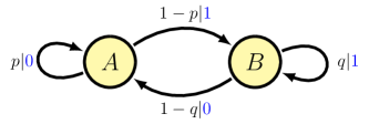
Figure 4: $\epsilon$-Machine generator of the Perturbed Coins Process. Edges are labeled with conditional transition probabilities and emitted symbols. For example, for the self-loop on state $A$, $p|{\color[rgb]{0,0,1}0}$ indicates the transition is taken with probability $\Pr({\color[rgb]{0,0,1}0}|A)=p$ and the symbol ${\color[rgb]{0,0,1}0}$ is emitted.

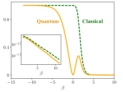
Figure 5: Classical memory $C_{\mu}(\beta)$ and quantum memory $C_{q}(\beta)$ versus $\beta$ for biased sampling of Perturbed Coins Process’ rare sequence classes: See Fig. 4, with $p=0.6$ and $q=0.8$. As the inset shows, for large $\beta$ both classical and quantum memories decay exponentially with $\beta$, but the quantum memory decays faster.

VII.1 Advantage for a Simple Markov Process

Consider the case where we have two biased coins, call them $A$ and $B$, and each has a different bias $p$ and $1-q$ both for Heads (symbol ${\color[rgb]{0,0,1}0}$), respectively. When we flip a coin, if the result is Heads, then on the next flip we choose coin $A$. If the result is Tails, we choose coin $B$. Flipping the coins over and over again results in a process $\mathcal{P}^{\text{pc}}$ called the Perturbed Coins Process [28]. Figure 4 shows the process’ $\epsilon$-machine generator $M(\mathcal{P}^{\text{pc}})$, where $\bm{\mathcal{S}}=\{A,B\}$ and $\mathcal{A}=\{0,1\}$.

One can also produce this process with a quantum generator $QM(\mathcal{P}^{\text{pc}})$. Using the construction introduced in Sec. IV, it has Kraus operators:

$$K_{0}\!=\!\frac{1}{d}\begin{bmatrix}\sqrt{q(1-q)p}-p\sqrt{1-p}&&p\sqrt{p}-(1-q)\sqrt{p}\\ \sqrt{q(1-q)(1-p)}-(1-p)\sqrt{(}p)&&p\sqrt{1-p}-(1-q)\sqrt{1-p}\end{bmatrix}$$

and:

$$K_{1}\!=\!\frac{1}{d}\begin{bmatrix}q\sqrt{(1-q)}-(1-p)\sqrt{1-q}&&\sqrt{p(1-p)(1-q)}-(1-q)\sqrt{q}\\ q\sqrt{(q)}-(1-p)\sqrt{(}q)&&\sqrt{p(1-p)q}-q\sqrt{1-q}\end{bmatrix}~{},$$

where $d=\sqrt{pq}+\sqrt{(1-p)(1-q)}$. For its stationary state distribution we have:

$$\rho_{s}=\frac{1}{2-p-q}\begin{bmatrix}&1-p&\alpha\\ &\alpha&1-q\end{bmatrix}~{},$$

where $\alpha=(1-q)\sqrt{p(1-p)}+(1-p)\sqrt{q(1-q)}$.

Figure 5 shows the classical and quantum memory costs to generate rare realizations: $C_{\mu}(\beta)$ and $C_{q}(\beta)$ versus $\beta$ for different $\beta$-classes. Surprisingly, the two costs exhibit completely different behaviors. For example, $\lim\limits_{\beta\to 0}C_{q}=0$, while $\lim\limits_{\beta\to 0}C_{\mu}=1$. More interestingly, as the inset demonstrates, even though both $C_{\mu}(\beta)$ and $C_{q}(\beta)$ vanish exponentially fast, in the limit of $\beta\to\infty$ $C_{q}(\beta)$ goes to zero noticeably faster.

We define the quantum advantage of biased sampling as the ratio of classical to quantum memory:

$$\eta(\beta)\equiv\frac{C_{\mu}(\beta)}{C_{q}(\beta)}~{}.$$

Figure 6 graphs the quantum advantage and shows how it divides into three distinct scaling regimes. First, for small $|\beta|$ (high-temperature) the quantum algorithm exhibits a polynomial advantage $\mathcal{O}(\beta^{-2})$. Second, for large positive $\beta$ (low-temperature) the quantum algorithm samples the rare classes with exponential advantage. The advantage grows as $\mathcal{O}(\exp{(c\beta}))$ as one increases $\beta$ and where $c$ is a function of $p$ and $q$. Third, for large negative $\beta$ (negative low-temperature regime) there is no quantum advantage. Since we are analyzing finite-state processes, this regime appears and is the analog of population inversion. And so, formally there are $\beta$-class events with negative temperature.

Such is the quantum advantage for the Perturbed Coins Process at $p=0.6$ and $q=0.8$. The features exhibited—the different scaling regimes—are generic for any $p>1-q$, though. Moreover, for Perturbed Coins Processes with $p<1-q$, the positive and negative low temperature behaviors switch.

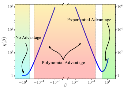
Figure 6: Quantum memory advantage for generating the rare realizations of the Perturbed Coins Process with $p=0.6$ and $q=0.8$ when employing its q-machine instead of it’s (classical) $\epsilon$-machine. Three different advantages occur: (i) near $\beta=0$ the polynomial advantage scales as $\mathcal{O}(\beta^{-2})$, (ii) large positive $\beta$, there is an exponential advantage $\mathcal{O}(\exp{(f(q,p)\beta}))$, and (iii) no advantage at large negative $\beta$.

VII.2 Spin System Quantum Advantage

Let us analyze the quantum advantage in a more familiar physics setting. Consider a general one-dimensional ferromagnetic next-nearest-neighbor Ising spin-½ chain [52, 53] defined by the Hamiltonian:

$$\mathcal{H}=-\sum_{i}\left(s_{i}s_{i+1}+\tfrac{1}{4}s_{i}s_{i+2}\right)~{},$$ (5)

in contact with thermal bath at temperature $k_{\textrm{B}}T=1$. The spin $s_{i}$ at site $i$ takes on values $\{+1,-1\}$.

After thermalizing, a spin configuration at one instant of time may be thought of as having been generated left-to-right (or equivalently right-to-left). The probability distribution over these spatial-translation invariant configurations defines a stationary stochastic process. Reference [54, Eqs. $(84)-(91)$] showed that for any finite and nonzero temperature $T$, this process has Markov order $2$. More to the point, the $\epsilon$-machine that generates this process has $4$ causal states and those states are in one-to-one correspondence with the set of length-$2$ spin configurations.

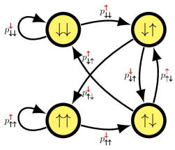
Figure 7: $\epsilon$-Machine that generates the spin configurations occurring in the one-dimensional ferromagnetic next-nearest-neighbor Ising spin chain with the Hamiltonian in Eq. (5).

Figure 7 displays the parametrized $\epsilon$-machine that generates this family of spin-configuration processes. To simulate the process, the generator need only remember the last two spins generated. This means the $\epsilon$-machine has four states, $\downarrow\downarrow$, $\downarrow\uparrow$, $\uparrow\downarrow$, and $\uparrow\uparrow$. If the last two observed spins are $\uparrow\uparrow$ for example, then the current state is $\uparrow\uparrow$. We denote the probability of generating a $\color[rgb]{1,0,0}\downarrow$ spin given that the previous two spins were $\uparrow\uparrow$ by $p^{{\color[rgb]{1,0,0}\boldsymbol{\downarrow}}}_{\boldsymbol{\uparrow\uparrow}}$. If the generator is in the $\uparrow\uparrow$ state and generates a $\color[rgb]{1,0,0}\downarrow$ spin, then the generator state changes to $\uparrow\downarrow$.

To determine the $\epsilon$-machine transition probabilities $\{T^{({x})}\}_{{x}\in\mathcal{A}}$, we first compute the transfer matrix $V$ for the Hamiltonian of Eq. (5) at temperature $T$ and then extract conditional probabilities, following Ref. [54] and Ref. [35]’s appendix.

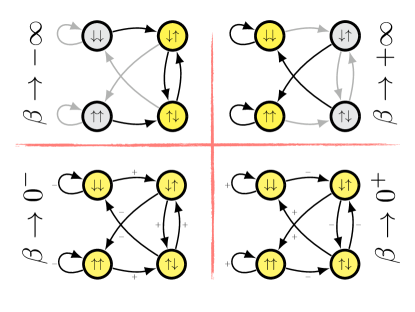
Figure 8: Classical generators of four important rare classes: (Top-left) Negative zero-temperature limit. (Top-right) positive zero temperature limit. (Bottom-left) Negative infinite temperature limit. (Bottom-right) positive temperature limit. Gray edges and states denotes them being rarely visited.

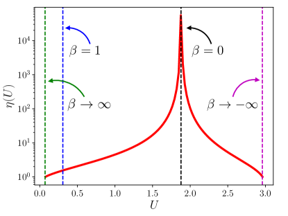
Figure 9: Quantum advantage for biased sampling of Ising spin configurations: $\eta(U)$ versus decay rate $U$ for bias sampling of equal-energy spin configurations. Vertical lines locate $\beta$s corresponding to particular $U$s. Note the extreme advantage indicated by the divergence in $\eta(U)$ at $U=u_{0}\approx 1.878$ corresponding to $\beta=0$.

What are the classical and quantum memory costs for bias sampling of the rare spin-configuration class with decay rate $U$, as defined in Eq. (3)? First, note that $U$ is not a configuration’s actual energy density. If we assume the system is in thermal equilibrium and thus exhibits a Boltzmann distribution over configurations, then $U$ and $E$ are related via:

$$U=\frac{\log_{2}(e)}{k_{\textrm{B}}T}(E-\mathcal{F}(T))~{},$$

where:

$$\mathcal{F}(T)=-k_{\textrm{B}}T\lim_{n\to\infty}\frac{1}{n}\ln\left(\sum_{\{w\in\mathcal{A}^{n}\}}e^{-\frac{nE(w)}{k_{\textrm{B}}T}}\right)~{}.$$

This simply tells us that if a stochastic process describes thermalized configurations of a physical system with some given Hamiltonian, then every rare-event bubble in Fig. 3 can be labeled either with $\beta$, $U$, or $E$. Moreover, there is a one-to-one mapping between every such variable pair.

Figure 9 plots $\eta(U)$ versus $U$—the quantum advantage of generating rare configurations with decay rate $U$. To calculate $\eta(U)$ for a given process $\mathcal{P}$, first we determine the process’ classical generator $M(\mathcal{P})$ using the method introduced in Ref. [33]. Second, for every $\beta\in\mathbb{R}/\{0\}$, using the map introduced in Sec. VI, we find the new classical generator $M(\mathcal{P}_{\beta})$. Third, using the construction introduced in Sec. III, we find $QM(\mathcal{P}_{\beta})$. Fourth, using Thm. 1 we find the corresponding $U$ for the chosen $\beta$. Using these results gives $\eta(U)=C_{\mu}(\beta)/C_{q}(\beta)$. By varying $\beta$ in the range $\mathbb{R}/\{0\}$ we cover all the energy density $U$s. Practically, to calculate $\eta(U)$ in Fig. (9), we chose $2000$ $\beta\in[-10,7.5]$.

As pointed out earlier, $\beta=1$ always corresponds to the process itself. And, one obtains its typical sequences. As one sees in Fig. 9, the quantum advantage $\eta(1)<2$. This simply means that, though there is a quantum advantage generating typical sequences, it is not that notable. However, the figure highlights four other interesting regimes.

First, there is the positive zero-temperature limit ($\beta\to\infty$) corresponding to the rare class with minimum energy density equal to $U_{\text{min}}=-\log_{2}(p^{{\color[rgb]{1,0,0}\boldsymbol{\downarrow}}}_{\boldsymbol{\downarrow\downarrow}})=-\log_{2}(p^{{\color[rgb]{1,0,0}\boldsymbol{\uparrow}}}_{\boldsymbol{\uparrow\uparrow}})$. From Eq. (5) it is easy to see that this rare bubble only has two configurations as members: all up-spins or all down-spins. Let us consider finite but large $\beta\gg 1$ that corresponds to the rare class with a low energy density close to $U_{\text{min}}$. Figure 8(top-left) shows a general $\epsilon$-machine for this process. Low color intensity for both edges and states means that the process rarely visits them during generation. This means, in turn, that a typical realization consists of large blocks of all up-spins and all down-spins. These large blocks are joined by small segments.

Second, there is the negative zero-temperature limit ($\beta\to-\infty$) that corresponds to the rare class with maximum energy density equal to $U_{\text{max}}=-\frac{1}{2}\log_{2}(p^{{\color[rgb]{1,0,0}\boldsymbol{\downarrow}}}_{\boldsymbol{\downarrow\uparrow}}p^{{\color[rgb]{1,0,0}\boldsymbol{\uparrow}}}_{\boldsymbol{\uparrow\downarrow}})$. From Eq. (5) it is easy to see that this rare bubble only has one configuration as a member: a periodic repetition of spin down and spin up. Consider finite $\beta\ll 1$ corresponding to a rare class with a high energy density close to $U_{\text{max}}$. Figure 8(top-right) shows the general $\epsilon$-machine for the associated process. The typical configuration consists of large blocks tiled with spin-up and spin-down pairs which are connected by other short segments.

Third, there is the positive infinite-temperature limit ($\beta\to 0^{+}$). In this limit we expect to see completely random spin-up/spin-down configurations. Figure 8(bottom-right) shows the $\epsilon$-machine for this class labeled with nonzero small $\beta$. The transition probability for the edges labeled $+$ is $\nicefrac{{1}}{{2}}+\epsilon$ and for the edges labeled $-$ is $\nicefrac{{1}}{{2}}-\epsilon$, where $\epsilon$ is a small positive number. As one can see, even though each transition probability is close to one-half, the self-loops are slightly favored.

Fourth and finally, there is the negative infinite-temperature limit ($\beta\to 0^{-}$). The generator here, Figure 8(bottom-left), is similar to that at positive infinite temperature, except that the edge-sign labels are reversed. This means that the self-loops are slightly less favored.

Generating a rare bubble with $\beta<0$ is sometimes called unphysical sampling since there exists no physical temperature at which the system generates this rare class. As a result, the left part of the Fig. 9 corresponds to physical sampling and the right part to unphysical sampling. That said, there is no impediment to “unphysical” sampling from a numerical standpoint. In addition, as we noted, negative temperatures correspond physically to population inversion, a well-known phenomenon.

Remarkably, the advantage $\eta(U)$ diverges at $U=u_{0}\approx 1.878$, where $u_{0}=\lim\limits_{\beta\to 0}U$— both the positive and negative high temperature limit. Moreover, the advantage $\eta(U)$ diverges as $(U-u_{0})^{-2}$ in both limits and, as a result, there is a polynomial-type advantage. For this specific example one does not find a region with exponential advantage.

VIII Conclusions

We introduced a new quantum algorithm for sampling the rare events of classical stochastic processes. The algorithm often confers a significant memory advantage when compared to the best known classical algorithm. We explored two example systems. In the first, a simple Markov process, we found that one gains either exponential or polynomial advantage. In the second, an Ising chain, we found a polynomial memory advantage for rare classes in both positive and negative high-temperature regimes.

Let us address an important point about the optimality of the classical and quantum algorithms. Consider the integer factorization problem. In this case Shor’s algorithm scales polynomially [24], while the best classical algorithm currently known scales exponentially [55] with problem size. While neither algorithm has been proven optimal, many believe that the separation in scaling is real [56]. Similarly, proving optimality for a rare-event sampling algorithm is challenging in both classical and quantum settings. However, with minor restrictions, one can show that the current quantum algorithm is almost always more efficient than the classical [29].

References

- [1] A. R. Leach. Molecular modelling: Principles and applications. Pearson Education, Boston, Massachusetts, 2001.
- [2] D. Frenkel and B. Smit. Understanding Molecular Simulation: From Algorithms to Applications. Academic Press, New York, second edition, 2007.
- [3] H. D. Miller. A convexity property in the theory of random variables defined on a finite Markov chain. An. Math. Stat., 32(4):1260–1270, 1961.
- [4] K. Young and J. P. Crutchfield. Fluctuation spectroscopy. Chaos, Solitons, and Fractals, 4:5 – 39, 1994.
- [5] V. Lecomte, C. Appert-Rolland, and F. van Wijland. Chaotic properties of systems with Markov dynamics. Phys. Rev. Lett., 95(1):010601, 2005.
- [6] V. Lecomte, C. Appert-Rolland, and F. Van Wijland. Thermodynamic formalism for systems with markov dynamics. J. Stat. Physics, 127(1):51–106, 2007.
- [7] R. Chetrite and H. Touchette. Nonequilibrium microcanonical and canonical ensembles and their equivalence. Phys. Rev. Lett., 111(12):120601, 2013.
- [8] S. R. S. Varadhan. Large deviations and applications. SIAM, Philadelphia, Pennsylvannia, 1984.
- [9] J. P. Garrahan, R. L. Jack, V. Lecomte, E. Pitard, K. van Duijvendijk, and F. van Wijland. First-order dynamical phase transition in models of glasses: an approach based on ensembles of histories. J. Phys. A: Math. Theo., 42(7):075007, 2009.
- [10] L. O. Hedges, R. L. Jack, J. P. Garrahan, and D. Chandler. Dynamic order-disorder in atomistic models of structural glass formers. Science, 323(5919):1309–1313, 2009.
- [11] J. Van Campenhout and T. M. Cover. Maximum entropy and conditional probability. IEEE Trans. Info. Th., 27(4):483–489, 1981.
- [12] I. Csiszár. Sanov property, generalized I-projection and a conditional limit theorem. Ann. Prob., 12(3):768–793, 1984.
- [13] G. M. Torrie and J. P. Valleau. Nonphysical sampling distributions in monte carlo free-energy estimation: Umbrella sampling. J. Comp. Physics, 23(2):187–199
- [14] S. Kumar, J. M. Rosenberg, D. Bouzida, R. H. Swendsen, and P. A. Kollman. The weighted histogram analysis method for free energy calculations on biomolecules. I. The method. J. Comp. Chemistry, 13(8):1011–1021
- [15] F. Wang and D. P. Landau. Efficient, multiple-range random walk algorithm to calculate the density of states. Phys. Rev. Let., 86(10):2050, 2001.
- [16] D. A. Levin, Y. Peres, and E. L. Wilmer. Markov Chains and Mixing Times. American Mathematical Society, Providence, Rhode Island, 2009.
- [17] J. R. Norris. Markov Chains, volume 2. Cambridge University Press, Cambridge, United Kingdom, 1998.
- [18] D. R. Upper. Theory and Algorithms for Hidden Markov Models and Generalized Hidden Markov Models. PhD thesis, University of California, Berkeley, 1997. Published by University Microfilms Intl, Ann Arbor, Michigan.
- [19] L. R. Rabiner and B. H. Juang. An introduction to hidden Markov models. IEEE ASSP Magazine, January, 1986.
- [20] L. R. Rabiner. A tutorial on hidden Markov models and selected applications in speech recognition. Proc. IEEE, 77(2):257–286
- [21] J. P. Crutchfield and D. P. Feldman. Regularities unseen, randomness observed: Levels of entropy convergence. CHAOS, 13(1):25–54, 2003.
- [22] J. P. Crutchfield. Between order and chaos. Nature Physics, 8(1):17–24, 2012.
- [23] J. P. Crutchfield and K. Young. Inferring statistical complexity. Phys. Rev. Let., 63:105–108, 1989.
- [24] P. W. Shor. Polynomial-time algorithms for prime factorization and discrete logarithms on a quantum computer. SIAM Review, 41(2):303–332
- [25] L. K. Grover. A fast quantum mechanical algorithm for database search. In Proceedings of the Twenty-Eighth Annual ACM Symposium on Theory of Computing, pages 212–219
- [26] D. S. Abrams and S. Lloyd. Quantum algorithm providing exponential speed increase for finding eigenvalues and eigenvectors. Phys. Rev. Let., 83(24):5162, 1999.
- [27] A. W. Harrow, A. Hassidim, and S. Lloyd. Quantum algorithm for linear systems of equations. Phys. Rev. Let., 103(15):150502, 2009.
- [28] M. Gu, K. Wiesner, E. Rieper, and V. Vedral. Quantum mechanics can reduce the complexity of classical models. Nature Comm., 3:762, 2012.
- [29] J. R. Mahoney, C. Aghamohammadi, and J. P. Crutchfield. Occam’s quantum strop: Synchronizing and compressing classical cryptic processes via a quantum channel. Sci. Reports, 6, 2016.
- [30] P. M. Riechers, J. R. Mahoney, C. Aghamohammadi, and J. P. Crutchfield. Minimized state complexity of quantum-encoded cryptic processes. Phys. Rev. A, 93(5):052317, 2016.
- [31] M. S. Palsson, M. Gu, J. Ho, H. M. Wiseman, and G. J. Pryde. Experimental quantum processing enhancement in modelling stochastic processes. arXiv:1602.05683, 2015.
- [32] N. F. Travers. Exponential bounds for convergence of entropy rate approximations in hidden markov models satisfying a path-mergeability condition. Stochastic Proc. Appln., 124(12):4149–4170, 2014.
- [33] C. R. Shalizi and J. P. Crutchfield. Computational mechanics: Pattern and prediction, structure and simplicity. J. Stat. Phys., 104:817–879, 2001.
- [34] G. Han and B. Marcus. Analyticity of entropy rate of hidden Markov chains. IEEE Trans. Info. Th., 52(12):5251–5266, 2006.
- [35] C. Aghamohammdi, J. R. Mahoney, and J. P. Crutchfield. Extreme quantum advantage when simulating strongly coupled classical systems. Sci. Reports, 7(6735):1–11, 2017.
- [36] A. J. P. Garner, Q. Liu, J. Thompson, V. Vedral, and M. Gu. Unbounded memory advantage in stochastic simulation using quantum mechanics. arXiv:1609.04408, 2016.
- [37] C. Aghamohammadi, J. R. Mahoney, and J. P. Crutchfield. The ambiguity of simplicity in quantum and classical simulation. Phys. Lett. A, 381(14):1223–1227, 2017.
- [38] J. Preskill. Lecture notes for physics 229: Quantum information and computation, volume 16. California Institute of Technology, Pasadena, California, 1998.
- [39] R. Durrett. Probability: theory and examples. Cambridge University Press, Cambridge, United Kingdom, 2010.
- [40] T. M. Cover and J. A. Thomas. Elements of Information Theory. Wiley-Interscience, New York, second edition, 2006.
- [41] S. Kullback. Information Theory and Statistics. Dover, New York, 1968.
- [42] R. W. Yeung. Information Theory and Network Coding. Springer, New York, 2008.
- [43] C. E. Shannon. A mathematical theory of communication. Bell Sys. Tech. J., 27:379–423, 623–656, 1948.
- [44] B. McMillan. The basic theorems of information theory. Ann. Math. Stat., 24:196–219, 1953.
- [45] L. Breiman. The individual ergodic theorem of information theory. Ann. Math. Statistics, 28(3):809–811, 1957.
- [46] L. Boltzmann. Lectures on gas theory. University of California Press, Berkeley, California, 1964.
- [47] H. Touchette. The large deviation approach to statistical mechanics. Physics Reports, 478:1–69, 2009.
- [48] C. Aghamohammadi and J. P. Crutchfield. Minimum memory for generating rare events. Phys. Rev. E, 95(3):032101, 2017.
- [49] R. L. Jack and P. Sollich. Large deviations and ensembles of trajectories in stochastic models. Prog. Theo. Physics Suppl., 184:304–317, 2010.
- [50] J. P. Garrahan and I. Lesanovsky. Thermodynamics of quantum jump trajectories. Phys. Rev. Lett., 104(16):160601, 2010.
- [51] R. Chetrite and H. Touchette. Nonequilibrium Markov processes conditioned on large deviations. In Annales Henri Poincaré, volume 16, pages 2005–2057. Springer, 2015.
- [52] R. J. Baxter. Exactly solved models in statistical mechanics. Academic Press, New York, New York, 2007.
- [53] A. Aghamohammadi, C. Aghamohammadi, and M. Khorrami. Externally driven one-dimensional Ising model. J. Stat. Mech., 2012(02):P02004
- [54] D. P. Feldman and J. P. Crutchfield. Discovering non-critical organization: Statistical mechanical, information theoretic, and computational views of patterns in simple one-dimensional spin systems. Santa Fe Institute, 1998. Santa Fe Institute Paper 98-04-026.
- [55] C. Pomerance. Fast, rigorous factorization and discrete logarithm algorithms. In Discrete Algo. Complexity, Proceedings of the Japan-US Joint Seminar, June 4-6, 1986, Kyoto, Japan, pages 119–143. Academic Press, New York, New York, 1987.
- [56] A. Bouland. Establishing quantum advantage. XRDS: Crossroads, The ACM Magazine for Students, 23(1):40–44