Statistical mechanics of coevolving spin system

Abstract

We propose a statistical mechanics approach to a coevolving spin system with an adaptive network of interactions. The dynamics of node states and network connections is driven by both spin configuration and network topology. We consider a Hamiltonian that merges the classical Ising model and the statistical theory of correlated random networks. As a result, we obtain rich phase diagrams with different phase transitions both in the state of nodes and in the graph topology. We argue that the coupling between the spin dynamics and the structure of the network is crucial in understanding the complex behavior of real-world systems and omitting one of the approaches renders the description incomplete.

During the last few decades, there has been a rapid development in the interdisciplinary area of network science. This may be because of the availability of vast amounts of data, much of it from such complex systems as financial markets, social and biological structures, and transportation networks. Studies of the network structure of such real-world systems as the World Wide Web Albert et al. (1999) indicate that their topology has numerous non-trivial properties that the classical random graph model cannot explain Erdös and Rényi (1959). This has produced new network models able to recreate some of these observed phenomena Watts and Strogatz (1998); Barabási and Albert (1999). Initially, most of these models focused on the graph evolution, often the growth in the number of nodes and edges Dorogovtsev and Mendes (2002). On the other hand, a different approach has been developed that considers a statistical ensemble of graphs Burda et al. (2001) called “exponential random graphs” Newman (2016). This formalism, borrowed from statistical physics, has proved successful and has led to a phenomenological theory of the topological phase transitions in evolving networks Burda and Krzywicki (2003); Berg and Lässig (2002); Palla et al. (2004).

This newly discovered concept of networks with a complex structure moved rapidly through the spin models community. Important critical properties were observed for both scale-free and small-world network versions of the canonical Ising model of ferromagnetism Herrero (2002); Aleksiejuk et al. (2002); Tadić et al. (2005). The use of complex networks became popular because they more closely resemble real-world structures than regular lattices or Poissonian graphs. This has been particularly important when modeling social and financial phenomena for which spin models are the simplest and the most common Sznajd-Weron and Sznajd (2000); Cont and Bouchaud (2000). Although the topology of many systems can be described using complex networks, the evolution of the model is limited to changes in the spin configuration. This implies that connection dynamics evolve more slowly than node state dynamics. Unfortunately, this assumption is not valid in most complex adaptive systems, which are describable using network tools. An Ising model with slowly evolving interactions was used as a model of a neural network Coolen et al. (1993) and as a possible tool for simulating magnetostriction in nanoscale magnetic structures Allahverdyan and Petrosyan (2006). A particularly interesting case involved models in which the connections and state dynamics coevolve with each other, one evolution depending on the other and resulting in non-trivial feedback. Most of these models focus on socio-economic systems and describe their dynamics Mandrà et al. (2009) rather than their statistical mechanics Biely et al. (2009); Toruniewska et al. (2016). Some of them produce intriguing topological properties, mainly when the dynamics is driven by the structural characteristics of the network Raducha and Gubiec (2017).

We here use the Hamiltonian formalism to describe Ising-like models with coevolution of spins and connections, and we want the connection dynamics to depend on both the spin configuration and network topology. Following the approach taken in Ref. Berg and Lässig (2002) we use the degree as a topological variable and focus on nearest neighbor interactions. We consider undirected graphs with a fixed number $N$ of vertices and a fixed number $M$ of edges. The partition function $Z$ for our ensemble we define to be

$$Z=\sum_{\{c_{ij}\},\{s_{i}\}}e^{-\beta H(\{c_{ij}\},\{s_{i}\})},$$ (1)

where $\{\cdot\}$ is all possible configurations with respect to a fixed number of links and nodes. Parameter $\beta$ is the strength of fluctuations and is the inverse temperature. A general form of the Hamiltonian that lies within the scope of this paper is

$$\begin{split}&H(\{c_{ij}\},\{s_{i}\})=\\ &\sum_{i<j}c_{ij}f(k_{i},k_{j},s_{i},s_{j})+\sum_{i}g(k_{i},s_{i}),\end{split}$$ (2)

where $c_{ij}$ is the adjacency matrix, $k_{i}=\sum_{j}c_{ij}$ and $s_{i}$ are respectively the degree and the spin of node $i$, and $f(\cdot)$ and $g(\cdot)$ are functions to be determined. More specifically, we assume that the functions are such that

$$\begin{split}&H(\{c_{ij}\},\{s_{i}\})=\\ &-\sum_{i<j}c_{ij}\left(\frac{k_{i}k_{j}}{\langle k\rangle}\right)^{\phi}s_{i}s_{j}-\sum_{i}k_{i}^{\gamma}-h\sum_{i}s_{i},\end{split}$$ (3)

where $\phi$ and $\gamma$ are model parameters, $\langle k\rangle=2M/N$, and $h$ is the external field acting on spins set to zero. This simple concrete form shows (i) that parameters $\phi$ and $\gamma$ allow us to continuously switch from complicated topological interactions to the classical Ising model, and (ii) that the multiplication of degrees is the simplest interaction expression. In an Ising framework, we treat it as a weight $J_{ij}$ assigned to an edge $(i,j)$. In addition, $J_{ij}=\left(\frac{k_{i}k_{j}}{\langle k\rangle}\right)^{\phi}$ is in accordance with real-world weighted network characteristics Barrat et al. (2004). The second sum term is an external field that interacts with each local node degree and drives the preference for high or low degree nodes. In addition to the classical ferromagnetic interpretation, if we use a socio-economic model to examine the proposed Hamiltonian we find an accurate interpretation of its terms. Using an opinion model we determine the influence of a given agent by examining its connectivity. The external field term forces each agent to reach as many people as possible. In contrast, the interaction term allows the energy of the system to be strongly affected by the connections among influential high degree nodes. This works in two ways. High-degree agents with opposite spins are energetically unstable, and agents with the same spins lower the energy level.

Figure 1: (Color online) Absolute magnetization $|m|$ (left) and the largest degree $k_{max}$ (right), as a function of the temperature $T=1/\beta$ and $\gamma$, for $\phi=0$. Solid line represents analytical approximation of the transition according to the equation (5). Results averaged over $5\cdot 10^{5}$ time steps for a network with $N=1000$ nodes and $M=3000$ edges.

Figure 2: (Color online) Absolute magnetization $|m|$, the largest degree $k_{max}$, and energy $E$ as a function of the temperature $T=1/\beta$, for $\gamma=1.6$ and $\phi=0$. Lines represent analytical approximations according to the equation (5) and symbols correspond to numerical simulations averaged over $10^{6}$ time steps for a network with $N=500$ (blue circles and solid line), $N=750$ (green squares and dotted line), $N=1000$ (red triangles and dashed line), with $c=M/N=3$. All quantities normalized to the range $[0,1]$, except the energy, which is given in arbitrary units.

The topological portion of the Hamiltonian changes the behavior of the Ising model. We find a variety of different effects. Some are structural, others are associated with spin configurations, and still others are a result of both. Figure 1 shows the simulation results for the phase diagram of $\gamma$ and $T$ with a fixed $\phi=0$. Here, no structural portion of the Hamiltonian describes interactions, i.e., the network structure is only locally important. Note that there are two separate topological phases and also a continuous phase transition in magnetization, with a small impact by parameter $\gamma$.

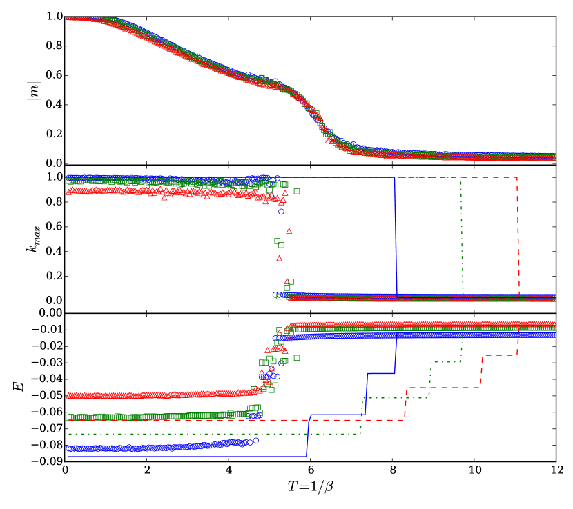
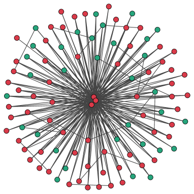
Figure 2 shows the case $\phi=0$ and $\gamma=1.6$. Note that the topological transition of the highest degree is discontinuous, but also that the magnetization behaves in a way similar to a standard Ising model on a coevolving network Biely et al. (2009). These effects belong to different transition classes and occur at different temperatures, and we see a striking behavior in energy $E$, i.e., the value of the Hamiltonian. It exhibits multiple jumps, one of which occurs at the same temperature as the highest-degree topological phase transition. In addition, all jumps are approximately equal. This energy behavior suggests a multi-star configuration in which the maximum number of stars is restricted by a fraction $\frac{M}{N}$. Figure 5(a) shows that when $M=3N$ three vertices are connected to approximately every network node. The number of stars decreases with the temperature. Eventually, the system becomes more homogeneous, and we see a sharp transition in the largest degree. Here $k_{\rm max}\ll N$, and the degree distribution is approximately Poissonian.

Figure 3: (Color online) Absolute magnetization $|m|$ (left) and the largest degree $k_{max}$ (right), as a function of the temperature $T=1/\beta$ and $\phi$, for $\gamma=1$. Solid and dashed lines represent analytical approximations of the transitions according to equations (7) and (8) respectively. Results averaged over $5\cdot 10^{5}$ time steps for a network with $N=1000$ nodes and $M=3000$ edges.

Figure 4: (Color online) Absolute magnetization $|m|$, the largest degree $k_{max}$, and energy $E$ as a function of the temperature $T=1/\beta$, for $\phi=0.6$ and $\gamma=1$. Lines represent analytical approximations according to the equation (7) and symbols correspond to numerical simulations averaged over $10^{6}$ time steps for a network with $N=500$ (blue circles and solid line), $N=750$ (green squares and dotted line), $N=1000$ (red triangles and dashed line), with $c=M/N=3$. All quantities normalized to the range $[0,1]$, except the energy, which is given in arbitrary units.

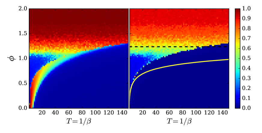
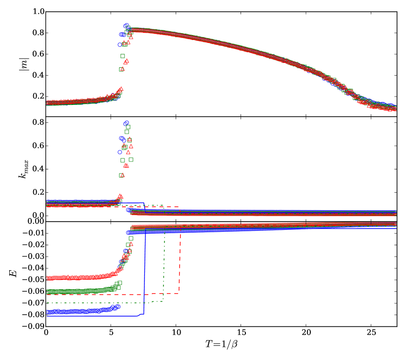
When we remove the external field associated with the degree of each node and turn on the combination of structural terms in the interaction portion of the Hamiltonian, we find a different behavior. Figure 3 shows this in the phase diagram with respect to $\phi$ and $T$ when there is a neutral value of $\gamma=1$. Figure 4 shows the same when we fix $\phi=0.6$. When we examine the largest degree and the magnetization we see four phases. Figure 4 shows that in the one-dimensional phase diagram the topological transition is characterized by a sharp jump in the maximum degree. Thus there is an abrupt change in the magnetization. Unlike the case with a varying $\gamma$, there is also a transition that is triggered by a change in parameter $\phi$, and that is unaffected by temperature. The critical value of $\phi$ in this transition is notated $\phi_{c}$.

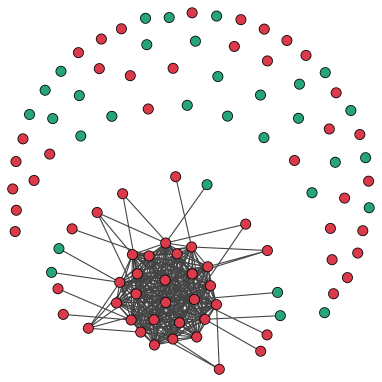
Examining the structural properties of the different phases mentioned above, we find that when $\gamma=1$ and $\phi<\phi_{c}$ in a low-temperature regime there are many disconnected nodes and one big component with high-degree clustering [see Fig. 5(b)]. At the critical temperature, the network recombines into one component, and the highest-degree $k_{\rm max}$ reaches its maximum value at the transition point. Increasing the temperature decreases the highest degree and the degree distribution to become Poissonian. When we increase $\phi$ above $\phi_{c}$, the system transitions into a multi-star configuration, a phase similar to the one previously observed for high $\gamma$ values.

(a) Model: $\phi=0$, $\gamma=2$

(b) Model: $\phi=1$, $\gamma=1$

Figure 5: (Color online) Exemplary networks obtained in the simulation. Green nodes indicate $+1$ spin, red nodes indicate $-1$ spin.

We next analytically describe the system to produce an approximation of our numerical results. Because the structural heterogeneity disallows a simple mean-field approach, we use a semi-mean-field method and focus on the non-homogeneous elements of the system that most strongly impact the Hamiltonian.

Figures 1 and 2 show the results when $\phi=0$ and the $\gamma$ value varies. We here assume that the most important part of the Hamiltonian is the contribution from the largest hubs, i.e., the stars connected to all other nodes. We assume non-hubs to have a degree equal to the average degree. Thus we approximate the Hamiltonian

$$H\approx-n_{h}k_{m}^{\gamma}-(N-n_{h})k^{\gamma}_{a},$$ (4)

where $n_{h}\in\{0,1,2,...,\lfloor\frac{M}{N}\rfloor\equiv\lfloor c\rfloor\}$ is the number of stars, $k_{m}=N-1$ is the degree of each star, $k_{a}$ is the average degree of the remaining nodes, and $k_{a}\equiv k_{a}(n_{h})=n_{h}+\frac{2(M-L(n_{h}))}{N-n_{h}}$, where $L(n_{h})=k_{m}+k_{m}-1+...+k_{m}-(n_{h}-1)=n_{h}\frac{2N-1-n_{h}}{2}$ is the number of links required to create $n_{h}$ stars. Taking into account all possible configurations, the partition function becomes

$$Z=2^{N}\sum_{n_{h}=0}^{\lfloor c\rfloor}\binom{N}{n_{h}}R(n_{h})e^{\beta[n_{h}k_{m}^{\gamma}+(N-n_{h})k^{\gamma}_{a}]},$$ (5)

where $2^{N}$ is all spin configurations, $\binom{N}{n_{h}}$ is the number of star combinations, and $R(n_{h})$ is the number of possible link configurations with $n_{h}$ stars in the network. We approximate this as $R(n_{h})\approx\binom{(N-n_{h})(N-n_{h}-1)/2}{M-L(n_{h})}$. Although this is a slight over-counting when $n_{h}<c$, the number of incorrect configurations is negligible when compared to the number of all other configurations.

Figures 1 and 2 show that the partition function allows us to analytically determine the energy and the highest degree. Although the estimated critical temperature diverges from the observed temperature, using this simple approach allows us to recreate the step-like behavior of the energy.

When $\gamma=1$ and the $\phi<\phi_{c}$ value varies, there is a shattering transition with a decreasing temperature. Some nodes disconnect from other nodes and become inactive. In contrast, when the temperature is high, and $c=3$, the graph becomes random and highly connected. Thus we describe the state of the system in terms of the number of active nodes, and we assume that their degree can be approximated using the mean field approach. We denote the number of these nodes $n_{s}$ and write the Hamiltonian

$$H\approx-M\frac{\langle k\rangle_{s}^{2\phi}}{\langle k\rangle^{\phi}},$$ (6)

where $\langle k\rangle_{s}=2M/n_{s}$ and $\lceil n_{\rm min}\rceil\leq n_{s}\leq N$ with $n_{\rm min}=(1+\sqrt{1+8M})/2$. We approximate the number of configurations for a particular $n_{s}$ with $\binom{N}{n_{s}}\binom{\frac{n_{s}(n_{s}-1)}{2}}{M}$ and derive the partition function

$$\begin{split}Z&=\sum_{n_{s}=\lceil n_{\min}\rceil}^{N}2^{N-n_{s}+1}\binom{N}{n_{s}}\times\\ &\times\binom{\frac{n_{s}(n_{s}-1)}{2}}{M}e^{\beta\,2^{\phi}\,N^{\phi}\,M^{\phi+1}\,n_{s}^{-2\phi}}.\end{split}$$ (7)

We assume that the spin direction of all active nodes is the same and that there are $2^{N-n_{s}+1}$ possible spin configurations. Figures 3 and 4 show the results when we analytically obtain the energy and the highest degree level. As in the previous case, we can use our estimation to approximate the system behavior, but not the critical temperature.

We approximate $\phi_{c}$ to fully describe the phase diagrams. The critical value of $\phi$ separates the homogeneous active node phase from the multi-star configuration phase. We assume that the energy of both phases is the same when $\phi=\phi_{c}$ and define the critical value

$$\begin{split}&\phi_{c}\ln\frac{(n_{\min}-1)^{2}}{N-1}+\ln\frac{M}{c}=\\ &\ln\left(\frac{c-1}{2}(N-1)^{\phi_{c}}+c^{\phi_{c}}(N-c)\right),\end{split}$$ (8)

where both $c$ and $n_{\rm min}$ retain the previous definitions. For the complete calculation of all cases see the Supplemental Material sup .

To statistically describe a coevolving spin system we have used a Hamiltonian that merges exponential random graphs and Ising-like models. A Hamiltonian that simultaneously depends on topological properties and node states has not been previously analyzed, and we have found complex behavior and have generated rich phase diagrams. The most striking aspect of our results is the existence, at specific temperatures, of topological phase transitions in which there are no node state transitions. There are also transitions that influence order parameters, but this suggests that we must take into account both the topology and the state of the nodes to fully describe the system, and if we do not we miss essential aspects of systemic behavior.

Although the results presented here concern networks in which $c\equiv\frac{M}{N}=3$, we did extend our simulations to other cases and found the same qualitative results. These extended results and a detailed analysis of the asymptotic and topological properties of the transitions will be supplied in a future publication Raducha and Wilinski (In preparation).

Acknowledgments: Mateusz Wilinski would like to acknowledge the support from the National Science Centre under Grant 2015/19/N/ST2/02701. Tomasz Raducha and Mateusz Wilinski would like to acknowledge the support from the Young Researchers of the Complex Systems Society under Bridge Grant 2018.

References

- Albert et al. (1999) R. Albert, H. Jeong, and A.-L. Barabási, nature 401, 130 (1999).
- Erdös and Rényi (1959) P. Erdös and A. Rényi, Publicationes Mathematicae (Debrecen) 6, 290 (1959).
- Watts and Strogatz (1998) D. J. Watts and S. H. Strogatz, nature 393, 440 (1998).
- Barabási and Albert (1999) A.-L. Barabási and R. Albert, science 286, 509 (1999).
- Dorogovtsev and Mendes (2002) S. N. Dorogovtsev and J. F. Mendes, Advances in physics 51, 1079 (2002).
- Burda et al. (2001) Z. Burda, J. D. Correia, and A. Krzywicki, Physical Review E 64, 046118 (2001).
- Newman (2016) M. Newman, pp. 565–588 (2016).
- Burda and Krzywicki (2003) Z. Burda and A. Krzywicki, Physical Review E 67, 046118 (2003).
- Berg and Lässig (2002) J. Berg and M. Lässig, Physical review letters 89, 228701 (2002).
- Palla et al. (2004) G. Palla, I. Derényi, I. Farkas, and T. Vicsek, Physical Review E 69, 046117 (2004).
- Herrero (2002) C. P. Herrero, Physical Review E 65, 066110 (2002).
- Aleksiejuk et al. (2002) A. Aleksiejuk, J. A. Hołyst, and D. Stauffer, Physica A: Statistical Mechanics and its Applications 310, 260 (2002).
- Tadić et al. (2005) B. Tadić, K. Malarz, and K. Kułakowski, Physical review letters 94, 137204 (2005).
- Sznajd-Weron and Sznajd (2000) K. Sznajd-Weron and J. Sznajd, International Journal of Modern Physics C 11, 1157 (2000).
- Cont and Bouchaud (2000) R. Cont and J.-P. Bouchaud, Macroeconomic dynamics 4, 170 (2000).
- Coolen et al. (1993) A. Coolen, R. Penney, and D. Sherrington, Physical Review B 48, 16116 (1993).
- Allahverdyan and Petrosyan (2006) A. Allahverdyan and K. Petrosyan, EPL (Europhysics Letters) 75, 908 (2006).
- Mandrà et al. (2009) S. Mandrà, S. Fortunato, and C. Castellano, Physical Review E 80, 056105 (2009).
- Biely et al. (2009) C. Biely, R. Hanel, and S. Thurner, The European Physical Journal B-Condensed Matter and Complex Systems 67, 285 (2009).
- Toruniewska et al. (2016) J. Toruniewska, K. Suchecki, and J. A. Hołyst, Physica A: Statistical Mechanics and its Applications 460, 1 (2016).
- Raducha and Gubiec (2017) T. Raducha and T. Gubiec, Physica A: Statistical Mechanics and its Applications (2017).
- Barrat et al. (2004) A. Barrat, M. Barthelemy, R. Pastor-Satorras, and A. Vespignani, Proceedings of the National Academy of Sciences of the United States of America 101, 3747 (2004).
- (23) See Supplemental Material at [URL to be inserted by publisher] for the formulas derivation and simulation details.
- Raducha and Wilinski (In preparation) T. Raducha and M. Wilinski (In preparation).