Global Sensitivity Analysis and Estimation of Model Error, Toward Uncertainty Quantification in Scramjet Computations
Abstract
The development of scramjet engines is an important research area for advancing hypersonic and orbital flights. Progress toward optimal engine designs requires accurate flow simulations together with uncertainty quantification. However, performing uncertainty quantification for scramjet simulations is challenging due to the large number of uncertain parameters involved and the high computational cost of flow simulations. These difficulties are addressed in this paper by developing practical uncertainty quantification algorithms and computational methods, and deploying them in the current study to large-eddy simulations of a jet in crossflow inside a simplified HIFiRE Direct Connect Rig scramjet combustor. First, global sensitivity analysis is conducted to identify influential uncertain input parameters, which can help reduce the system’s stochastic dimension. Second, because models of different fidelity are used in the overall uncertainty quantification assessment, a framework for quantifying and propagating the uncertainty due to model error is presented. These methods are demonstrated on a nonreacting jet-in-crossflow test problem in a simplified scramjet geometry, with parameter space up to 24 dimensions, using static and dynamic treatments of the turbulence subgrid model, and with two-dimensional and three-dimensional geometries.
Nomenclature
| = | modified Smagorinsky constant | |
| = | solution to the reduced least absolute shrinkage and selection operator problem | |
| = | coefficient for the th basis function | |
| = | data set | |
| = | injector diameter, mm | |
| = | cross-validation error | |
| = | low-fidelity model | |
| = | quantity of interest (model output) | |
| = | quantity of interest from a model with discretization level | |
| = | ||
| = | surrogate model for | |
| = | approximations to and | |
| = | regression matrix, solution vector, and right-hand-side vector | |
| = | and with rows corresponding to the th subset only | |
| = | and with rows corresponding to the th subset removed |
| = | high-fidelity model | |
| = | inlet and fuel turbulence intensity magnitudes | |
| = | index set | |
| = | Gaussian approximation to the marginalized likelihood | |
| = | inlet and fuel turbulence length scales, mm | |
| = | discretization level | |
| = | inlet and fuel Mach numbers | |
| = | fuel mass flux, kg/s | |
| = | independent and identically distributed as normal distribution with mean | |
| and variance | ||
| = | stochastic dimension | |
| = | root-mean-square static pressure | |
| = | stagnation pressure | |
| = | turbulent Prandtl number | |
| = | polynomial degree | |
| = | probability density function | |
| = | inlet stagnation pressure, MPa | |
| = | stochastic model | |
| = | validation residual to the reduced least absolute shrinkage and selection | |
| operator problem | ||
| = | turbulent Schmidt number | |
| = | main effect Sobol sensitivity index for the th input parameter | |
| = | joint effect Sobol sensitivity index for the interaction of th and th input | |
| parameters | ||
| = | total effect Sobol sensitivity index for all terms involving the th input parameter | |
| = | shared continuous operating conditions | |
| = | fuel static temperature, K | |
| = | wall temperature | |
| = | inlet stagnation temperature, K | |
| = | distributed as uniform distribution from to | |
| = | streamwise, wall-normal, and spanwise coordinates, mm | |
| = | streamwise, wall-normal, and spanwise coordinates normalized by injector diameter | |
| = | ethylene mass fraction | |
| = | mixture fraction | |
| = | parameter of | |
| = | combined parameters and | |
| = | multi-index | |
| = | inlet boundary layer thickness, mm | |
| = | model discrepancy term | |
| = | surrogate model error | |
| = | least absolute shrinkage and selection operator regularization parameter | |
| = | model input parameter vector | |
| = | th component of , all components of except the th | |
| = | expansion coefficients | |
| = | mean | |
| = | support of | |
| = | independent and identically distributed basic (germ) random variables | |
| = | th regression point |
| = | multiplicative term | |
| = | standard deviation, variance | |
| = | scalar dissipation rate | |
| = | multivariate and univariate orthonormal polynomial basis functions | |
| = | th basis function |
1 Introduction
Supersonic combustion ramjet (scramjet) engines allow propulsion systems to transition from supersonic to hypersonic flight conditions while ensuring stable combustion, potentially offering much higher efficiencies compared to traditional technologies such as rockets or turbojets. While several scramjet designs have been conceived, none to date operate optimally [60]. This is due to difficulties in characterizing and predicting combustion properties under extreme flow conditions, coupled with multiscale and multiphysics nature of the processes involved. Designing an optimal engine involves maximizing combustion efficiency while minimizing pressure losses, thermal loading, and the risk of “unstart” or flame blowout. Achieving this, especially in the presence of uncertainty, is an extremely challenging undertaking.
An important step towards optimal scramjet design is to conduct accurate flow simulations together with uncertainty quantification (UQ). While UQ in general has received substantial attention in the past decades, UQ for scramjet applications is largely undeveloped, with a few exceptions [65, 4]. A comprehensive UQ study in such systems has been prohibitive due to both the large number of uncertainty sources in the predictive models as well as the high computational cost of simulating multidimensional turbulent reacting flows. This study aims to advance practical algorithms and computational methods that enable tractable UQ analysis of realistic scramjet designs. The immediate goals are to:
-
1.
focus on an initial nonreacting jet-in-crossflow test problem in a simplified scramjet geometry;
-
2.
identify influential uncertain input parameters via global sensitivity analysis, which can help reduce the system’s stochastic dimension;
-
3.
quantify and propagate the uncertainty due to model error from using low-fidelity models; and
-
4.
demonstrate these UQ methods on the jet-in-crossflow problem (nonreacting, simplified scramjet geometry), and prepare extensions to its full configuration.
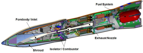
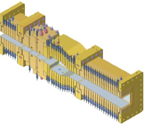
We concentrate on a scramjet configuration studied under the HIFiRE (Hypersonic International Flight Research and Experimentation) program [5, 6], which has been the target of a mature experimental campaign with accessible data through its HIFiRE Flight 2 (HF2) project [29, 30]. The HF2 payload, depicted in Fig. 1(a), involves a cavity-based hydrocarbon-fueled dual-mode scramjet that enables transition from ramjet mode (subsonic flow in the combustor) to scramjet mode (supersonic flow in the combustor) through a variable Mach number flight trajectory. The isolator/combustor was derived from a series of legacy configurations at the U.S. Air Force Research Laboratory [23, 30], whereas the forebody, inlet, and nozzle were designed at NASA Langley Research Center [12, 22]. A ground test rig, designated the HIFiRE Direct Connect Rig (HDCR, Fig. 1(b)), was developed to duplicate the isolator/combustor layout of the flight test hardware and to provide ground-based data for comparisons with flight data, verifying engine performance and operability as well as designing fuel delivery schedule [26, 63]. Mirroring the HDCR setup, we aim to simulate and assess flow characteristics inside the isolator/combustor portion of the scramjet.
The paper is structured as follows. Section 2 describes the physics and solver used for simulating the jet in crossflow inside the simplified HDCR scramjet combustor, in particular with the use of large-eddy simulation techniques. We then introduce global sensitivity analysis in Sec. 3 to identify the most influential input parameters of the model. In Sec. 4, a framework is presented to capture uncertainty from model error when low-fidelity models are used. These UQ methods are then demonstrated on the jet-in-crossflow problem, with results shown in Sec. 5. Finally, the paper ends with conclusions and future work discussions in Sec. 6.
2 Large-Eddy Simulations for the HIFiRE Direct Connect Rig
2.1 Computational domain
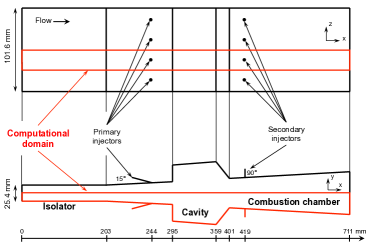
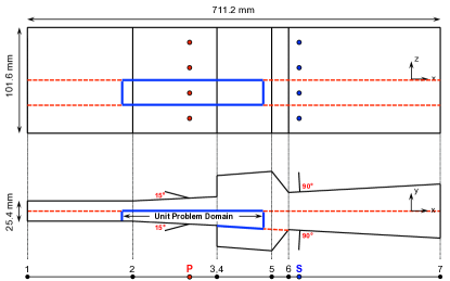
We aim to perform flow simulations inside the HDCR. A detailed schematic of the HDCR geometry is shown in Fig. 2(a). The rig consists of a constant-area isolator (i.e., planar duct) attached to a combustion chamber. It includes four primary injectors that are mounted upstream of flame stabilization cavities on both the top and bottom walls. Four secondary injectors along both walls are also positioned downstream of the cavities. Flow travels from left to right in the -direction (streamwise), and the geometry is symmetric about the centerlines in both the -direction (wall-normal) and -direction (spanwise). Numerical simulations can take advantage of this symmetry by considering a domain that comprises only the bottom half and one set of the primary and secondary injectors. This “full” computational domain is highlighted by red lines in Fig. 2(a).
Even with symmetry-based size reductions of the computational domain, the cost associated with the thousands of simulations required for UQ analysis necessitates further simplifications. Since the current focal point is to develop, validate, and demonstrate the various UQ methodologies, a unit test problem is designed for these purposes. Calculations are performed in the region near the primary injectors along the bottom wall ( to 350 mm). The domain is simplified by considering only a single primary injector and omitting the presence of the cavity. Chemistry is initially disabled, allowing a targeted investigation of the interaction between the fuel jet (JP-7 surrogate: 36% methane and 64% ethylene) and the supersonic crossflow without the effects of combustion reaction. The location of the outflow boundary is chosen to ensure the flow to be fully supersonic across the entire exit plane. The computational domain for the unit test problem is identified by the solid blue lines in Fig. 2(b). The flow conditions of interest correspond to the freestream and fuel injection parameters reported by the HDCR experiments. Details related to large-eddy simulation of the full HDCR configuration are described by Lacaze et al. [36].
2.2 Large-eddy simulation solver: RAPTOR
Large-eddy simulation (LES) calculations are performed using the RAPTOR code framework developed by Oefelein [42, 41]. The solver has been optimized to meet the strict algorithmic requirements imposed by the LES formalism. The theoretical framework solves the fully coupled conservation equations of mass, momentum, total-energy, and species for a chemically reacting flow. It is designed to handle high Reynolds number, high-pressure, real-gas and/or liquid conditions over a wide Mach operating range. It also accounts for detailed thermodynamics and transport processes at the molecular level. Noteworthy is that RAPTOR is designed specifically for LES using non-dissipative, discretely conservative, staggered, finite-volume differencing. This eliminates numerical contamination of the subfilter models due to artificial dissipation and provides discrete conservation of mass, momentum, energy, and species, which is imperative for high quality LES. Representative results and case studies using RAPTOR can be found in studies by Oefelein et al. [47, 46, 44, 43, 45], Williams et al. [64], Lacaze et al. [35], and Khalil et al. [34].
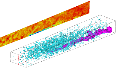
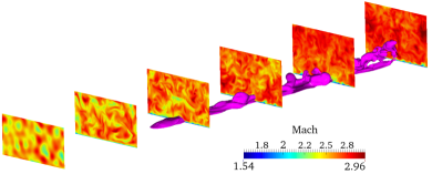
Sample results for the jet-in-crossflow problem are presented in Fig. 3. Here, the instantaneous Mach number is shown across different planes along with isocontours of ethylene (fuel component) mass fraction and -criterion contours that highlight coherent turbulent structures.
3 Global Sensitivity Analysis
UQ encompasses many different investigations (e.g., uncertainty propagation, optimal experimental design, model calibration, optimization under uncertainty); we start by introducing global sensitivity analysis (GSA) [56, 55] in this paper. GSA provides insights on the behavior of uncertainty of model output quantities of interest (QOIs), and identifies input parameters that are unimportant to these QOIs, which may be subsequently eliminated—i.e., it is useful for dimension reduction of the input space. GSA achieves this by quantifying the importance of each uncertain input parameter with respect to the predictive uncertainty of a given QOI. In contrast to local sensitivity analysis, GSA reflects the overall sensitivity characteristics across the entire input domain.
We focus on variance-based properties of the input and output variables. Loosely speaking, variance of a QOI can be decomposed into contributions from the uncertainty of each input parameter. Let denote the vector of all input parameters; we compute Sobol sensitivity indices [62] to rank the components in terms of their variance contributions to a given QOI :
-
•
Main effect sensitivity measures variance contribution solely due to the th parameter:
(1) The notation refers to all components of except the th component.
-
•
Joint effect sensitivity measures variance contribution from the interaction of th and th parameters:
(2) -
•
Total effect sensitivity measures variance contributions from all terms that involve the th parameter:
(3)
Total effect sensitivity is particularly informative for identifying parameters that have the highest overall impact on the QOI. The unimportant parameters, for example, then may be fixed at their nominal values without significantly underrepresenting the QOI variance. Subsequently, the stochastic input dimension would be reduced at a cost of only small variance approximation errors. The primary objective of the GSA study in this paper is to compute the total effect sensitivity indices.
Traditionally, sensitivity indices are directly estimated via various flavors of efficient Monte Carlo (MC) methods [61, 32, 57, 53, 54]. The number of samples needed, however, is typically impractical when expensive models (such as LES) are involved. We tackle this difficulty via two approaches. First, we take advantage of multilevel (ML) and multifidelity (MF) formulations, to construct QOI approximations by combining simulation from models of different discretization levels (e.g., grid resolutions) and fidelity (i.e., modeling assumptions). These frameworks help transfer some of the computational burden from expensive models to inexpensive ones, and reduce the overall sampling cost. In particular, a control-variate-based MLMF Monte Carlo (MLMF MC) method is used to produce efficient sample allocation across different models. Second, we adopt polynomial chaos expansions (PCEs) to approximate the QOIs in ML and MF forms, thereby presuming a certain degree of smoothness in the QOIs, with attendant computational savings for given accuracy requirements. Additionally, compressed sensing (CS) is used to discover sparse PCE structures from small numbers of model evaluations. Once these PCEs become available, their orthogonal polynomial basis functions allow Sobol indices to be extracted analytically from expansion coefficients without the need of additional MC sampling.
Figure 4 shows a summary of the computational concepts and tools used for GSA, and may serve as a useful reference for readers as they are introduced later.
3.1 Multilevel and multifidelity representations
Performing UQ directly on the highest fidelity model available is usually very challenging, if not altogether intractable, due to its high simulation cost. Often, models employing different discretization levels and modeling assumptions are also available, and even those with coarse grids and low fidelity can provide some information about the output behavior. It would be useful to then extract information from inexpensive simulations whenever possible, and resort to expensive ones for details that can only be characterized through those models. We thus seek multimodel approaches that are more efficient overall, and specifically focus on ML and MF representations.
We start by first describing the ML concept. Consider a generic QOI produced by a model with discretization level (e.g., grid resolution) , denoted by , and and are the coarsest and finest available resolutions, respectively. The QOI from the finest resolution can be expanded exactly as
| (4) |
where denotes the difference terms on adjacent levels. One motivation behind using this telescopic decomposition is that can become better behaved and easier to characterize than the QOI directly as some of the nonlinear behavior may be subtracted out. One can also view this as an exploitation of the correlation between evaluations at different levels, where information injected from the inexpensive simulations help reduce the need to evaluate expensive models, and thus decrease the overall cost of characterizing .
From here, the expansion can be utilized in a few different ways; we focus on its use for uncertainty propagation. For example, one may take expectations with respect to on each term, and generate MC samples to obtain efficient moment estimators of the finest-resolution QOI. This is known as the ML Monte Carlo method and has extensive theoretical developments stemming from the work of Giles [20]. Alternatively, one may be interested in producing functional approximations of the QOI response:
| (5) |
where and are approximations to and , respectively. We take this path, and adopt PCEs (see next section) for these approximations. One motivation for this choice is that we want to leverage the observed smoothness of QOIs over the parameter space. Another reason is that the resulting PCEs provide a convenient form in which GSA may be performed, and the PCEs can also be reused in other UQ investigations within the overall project.
An analogous argument can be made across models of different fidelity, and we refer to this parallel expansion as the MF form. The analysis of MF approaches can be more difficult than ML, since differences induced by modeling assumptions are more challenging to characterize systematically, and no longer rely on properties resulting from the convergence of grid resolution. Nonetheless, MF remains a valuable tool, and has been initially explored with the use of sparse grids [40, 9]. A comprehensive survey regarding MF methods can be found in a report by Peherstorfer et al. [49].
With details in the subsequent section, we proceed to use a sample-based regression approach to construct the approximations and . The allocation of samples evaluated at different levels and fidelity are computed using the MLMF MC method [15, 16]. This algorithm applies a MF control variate to an ML expansion, and generates a sample allocation that minimizes the variance of the overall MC estimator, which, at the same time, also accounts for the computational cost of model simulations. While this allocation procedure provides an optimal-variance MC estimator, it is not directly aimed for an optimal construction of the approximation functions. However, they still provide a good general sample allocation that is useful for our study here. Once and become available, the overall approximation can be recovered by adding them according to Eqn. 5.
3.2 Polynomial chaos expansion
PCEs are used to approximate the terms in Eqn. 5. A PCE is a spectral representation of a random variable. It provides a useful means for propagating uncertainty as an alternative to MC simulations. We provide a brief description of PCE below, and refer readers to several books and review papers for detailed discussions [19, 38, 66, 37].
With mild technical assumptions [10], a real-valued random variable with finite variance (such as an uncertain input parameter) can be expanded in the following form:
| (6) |
where are independent and identically distributed (i.i.d.) basic (germ) random variables; is the stochastic dimension (often chosen to equal the system stochastic degrees of freedom for convenience, though Eqn. 6 can hold for any finite or infinite with associated requirements [10]); are the expansion coefficients; , is a multi-index; and are multivariate normalized orthogonal polynomials written as products of univariate orthonormal polynomials
| (7) |
The univariate functions are polynomials of degree in the independent variable , and orthonormal with respect to the density of (i.e., ):
| (8) |
where is the support of . Different choices of and under the generalized Askey family are available [67]. We employ uniform and Legendre polynomials in this study. In practice, the infinite sum in the expansion Eqn. 6 is truncated:
| (9) |
where is some finite index set. For example, one popular choice for is the “total-order” expansion of degree , where . Similarly, we can write the PCE for a QOI in the form
| (10) |
Methods for computing its coefficients are broadly divided into two groups: intrusive and non-intrusive. The former involves substituting the expansions directly into the governing equations and applying Galerkin projection, resulting in a larger, new system for the PCE coefficients that needs to be solved only once. The latter involves finding an approximation in the subspace spanned by the basis functions, which typically requires evaluating the original model many times. With our model only available as a black box in practice, and also to accommodate flexible choices of QOIs that may be complicated functions of the state variables, we elect to take the non-intrusive route.
One non-intrusive method relies on Galerkin projection of the solution, known as the non-intrusive spectral projection (NISP) method:
| (11) |
Generally, the integral must be estimated numerically and approximately via, for example, sparse quadrature [1, 17, 18]. When the dimension of is high, model is expensive, and only few evaluations are available, however, even sparse quadrature becomes impractical. In these situations, regression is a more effective method, which involves solving the following regression linear system :
| (12) |
where refers to the th basis function, is the coefficient corresponding to that term, and is the th regression (training) point. is thus the regression matrix where each column corresponds to a basis term and each row corresponds to a regression point.
For LES, the affordable number of simulations is expected to be drastically smaller than the number of basis terms , leading to an extremely underdetermined system. For example, a total-order expansion of degree 3 in 24 dimensions contains terms, while 2925 of 3D LES with a moderate grid resolution (i.e., each grid cell is the size of the injector diameter mm) would take more than 64 million CPU hours! While ML and MF formulations help reduce the number of expensive model simulations, we also utilize CS (see next section) to discover sparse structure in the PCE and remove basis terms with low magnitude coefficients. Once the final PCE for the QOI is established, we can extract the Sobol indices via the formulae:
| (13) | ||||
| (14) | ||||
| (15) |
and the QOI variance can be computed by
| (16) |
3.3 Compressed sensing
CS [2, 7] aims to recover sparse solutions of underdetermined linear systems, and its use for finding sparse PCEs in the presence of limited data has received considerable attention within the UQ community in recent years [51, 25, 11, 50, 9, 59, 31, 28]. Typically, this entails finding the solution with the fewest number of non-zero components—i.e., minimizing its -norm. However, -minimization is an NP-hard problem [39]. A simpler convex relaxation minimizing the -norm minimization is often used as an approximation, and is proven to uniquely achieve the solution in the limit of large systems and when the true solution is sufficiently sparse [8]. We focus on one variant of -sparse recovery—the (unconstrained) least absolute shrinkage and selection operator (LASSO) problem:
| (17) |
where is a scalar regularization parameter. We demonstrate one possible method for solving the LASSO problem (other algorithms were explored as well but omitted for brevity) through the gradient projection for sparse reconstruction (GPSR) [13]. GPSR targets Eqn. 17 by employing a positive-negative split of the solution vector, yielding a quadratic program in the resulting new form. A gradient descent with backtracking is then performed, and constraints are handled by projection onto the feasible space. For our numerical demonstrations, we use the MATLAB implementation GPSR v6.0 from the developers’ website [14].
By promoting sparsity, CS is designed to reduce overfitting. An overfit solution is observed when the error on training set (i.e., data used to define the underdetermined linear system) is very different (much smaller) than error on a separate validation set, and the use of a different training set could lead to entirely different results. Such a solution has poor predictive capability and thus unreliable. CS is not always successful in preventing overfitting, such as when in Eqn. 17 is poorly chosen. reflects the relative importance between the and terms; the former represents regularization and smoothing, and the latter for producing predictions that closely match the training data. A large heavily penalizes nonzero terms of the solution vector, forcing them toward zero (underfitting); a small emphasizes data fit, and may lead to solutions that are not sparse, and that only fit the training points but otherwise do not predict well (overfitting). A useful solution thus requires an intricate selection of , which is a problem-dependent and nontrivial task. We examine and control the degree of overfitting by employing cross-validation (CV) [27] to guide the choice of . In particular, we use the -fold CV error. The procedure involves first partitioning the full set of training points into (approximately) equal subsets. For each of the subsets, a reduced version of the original LASSO problem is solved:
| (18) |
where denotes but with rows corresponding the th subset removed, is with elements corresponding to the th subset removed, and is the solution vector from solving this reduced problem. The residual from validation using the th subset that was left out is therefore
| (19) |
where denotes that only contains rows corresponding to the th subset, and is containing only elements corresponding to the th subset. Combining the residuals from repeating the exercise on all subsets, we arrive at the (normalized) -fold CV error
| (20) |
The CV error thus provides an estimate of the validation error using only the training data set at hand and without needing additional validation points, and reflects the solution predictive capability. The CS problem with selection through CV error is:
| (21) | |||
| (22) |
Note that solving Eqn. 22 does not require the solution from the full linear system, only the reduced systems. can be found by, for example, a grid search across the -space.
4 Embedded Representation of Model Error
Classical Bayesian model calibration typically assumes that data are consistently generated from the model—that is, the model is correct. In reality, all models are approximations to the truth, and different models trade off between accuracy and computational cost with their assumptions and parameterizations. For example, computational studies of turbulent combustion may employ different geometry details, flow characteristics, turbulence modeling, grid resolutions, and even the inclusion or removal of entire physical dimensions. As we make use of different models, it is crucial not only to acknowledge and understand—but also to develop the capability to represent, quantify, attribute, and propagate—the uncertainty due to model error. We address model error in this study by focusing on the quantities we ultimately care about in an engineering context: model predictions.
Consider two models: a high-fidelity model and a low-fidelity model . Both models are functions of shared continuous operating conditions , which in the context of the current LES studies consist of the spatial coordinates. The low-fidelity model also carries parameters , which may be calibrated to provide requisite “tuning” of the model and potentially providing some compensation for its lower fidelity. Furthermore, component notations and denote the th model observable (i.e., the categorical model output variable, such as temperature, pressure, etc.). We are interested in the uncertainty incurred in predictive QOIs when is used in place of . This entails first the calibration of the low-fidelity model using data from the high-fidelity model .
We approach the calibration problem taking a Bayesian perspective. Kennedy and O’Hagan [33] pioneered a systematic Bayesian framework for characterizing model error, by employing a linear stochastic model , with the calibration data interpreted as sample realizations of . This form uses an additive Gaussian process model discrepancy term , and is a constant factor. While this approach is quite flexible in terms of attaining good fits for each calibration quantity, it presents difficulties when certain physical properties are desired in the predictions. First, the multiplicative and additive structures generally cannot guarantee the predictive quantity to maintain satisfaction of the underlying governing equations and physical laws instituted in . Second, the discrepancy term, , is not transferable for prediction of variables outside those used for calibration (i.e., for predicting with ).
Alternative approaches have been introduced in recent years that target the aforementioned difficulties. For example, Sargsyan et al. [58] take a non-intrusive approach and embed a stochastic variable that represents model discrepancy in the low-fidelity model parameters, while Oliver et al. [48] elect to include a correction term on less-reliable embedded models that exist within a highly-reliable set of governing equations. We adopt the approach of Sargsyan et al. [58], first embedding the discrepancy term in the model parameters such that , then employing a parametric stochastic representation to arrive at the following characterization of the high-fidelity data behavior:
| (23) |
Here, is a parameter of , and is a fixed random variable such as a standard normal. The uncertainty due to model error is thus encoded in both the distributions of and , where the former is reducible and can be learned from data while the latter remains fixed. In this form, the predictive quantity automatically preserves physical laws imposed in to the extent that this random perturbation of is within physical bounds. Furthermore, while remains specific to the th observable, we expect it to be better behaved, and generally more meaningful when extrapolated to other observables. This is supported by the fact that is now a correction term to the same parameter regardless of , and would always remain in the same physical unit and likely similar magnitude. In contrast, the additive from Kennedy and O’Hagan would be under entirely different physical units and potentially orders-of-magnitude different across different .444Another known difficulty with the external additive model error is the non-idenfiability between model error and measurement noise contributions: there can be (possibly infinite) different combinations of model discrepancy and data noise that together characterize the overall data distribution. The embedded form in Eqn. 23 would be able to better separate and distinguish the model error (internal) and data noise (external). As discussed in Footnotes 6 and 7 from Sec. 5, one source of data noise in this paper’s numerical examples is the variation due to time averaging. However, this variation is observed to be very small compared to uncertainty contributions from model error and parameter posterior. We thus do not include them in the equations and numerical results presented, and also do not demonstrate the separation of data noise in the embedded representation. Nonetheless, extrapolation of is still needed for prediction. Finding the relationship of model error across different observables is a challenging task. We take a reasonable first step and use a constant extrapolation, by assuming to be the same across space (thus it is now a random variable rather than a random process), and also across all observables , leading to
| (24) |
Finally, for simplifying notation, is assumed to be discretized with nodes , and the overall model output vector thus has the form
| (25) |
where is the combined index of and .
In this study, we choose to represent the randomly perturbed parameter as a Legendre-Uniform PCE:
| (26) |
where are Legendre polynomial functions. We use uniform distributions to better control the range of the perturbed parameter, though other PCE variants (e.g., Gauss-Hermite) are possible as well. When is multi-dimensional, the different components of may use different orders of expansions. In practice, we may choose to embed in certain targeted parameter components, while keeping others at zeroth-order (i.e., treated in the classical Bayesian manner). In the numerical examples of this paper, linear expansions are used for the embedded components. A demonstration of choosing the embedding components will be shown in the numerical results. The full set of parameters to be calibrated is grouped together via the notation . The model calibration problem thus involves finding the posterior distribution on via Bayes’ theorem
| (27) |
where is the set of calibration data points (which are the high-fidelity model evaluations in this case), is the prior distribution, is the likelihood function, and is the evidence. The prior and posterior represent our states of knowledge about the uncertainty in the parameters before and after the data set is assimilated. To facilitate Bayesian inference and obtain the posterior in a practical manner, we will further develop the likelihood model below. Once the posterior is characterized, it can be subsequently propagated through the low-fidelity model to obtain posterior predictive distributions on the desired QOIs—that is, predictions that account for both model error and parameter uncertainty.
Figure 5 shows a summary of the computational concepts and tools used for the embedded model error representation, and may serve as a useful reference for readers as they are introduced below.
4.1 Surrogate for low-fidelity model
Under this framework, the high-fidelity model only needs to be evaluated to generate data for Bayesian inference; this typically involves a small number of evaluations. The low-fidelity model, however, needs to be run as many times as is required to perform Bayesian inference in characterizing the posterior ; this entails a much larger number of evaluations in comparison. When the low-fidelity model evaluations are still expensive, a surrogate model is needed. We proceed to build a surrogate using Legendre polynomials for each QOI involved in either calibration or prediction, , as functions of the overall input argument , to replace the low-fidelity model. The approximation error is represented with an additive Gaussian form, and so Eqn. 25 becomes
| (28) |
where is the surrogate to the low-fidelity model, and encapsulates the error of the surrogate with respect to the low-fidelity model. In this study, it is assumed and independent of the surrogate model input (but depends on ). The variance terms are the leave-one-out cross-validation errors from the linear regression systems used for constructing the surrogates, and can be computed analytically and quickly (e.g., [3]). We emphasize that is still representing the model discrepancy between the high-fidelity and low-fidelity models, not between the high-fidelity and the surrogate models.
4.2 Likelihood approximation
We characterize the posterior via Markov chain Monte Carlo sampling [21, 52], specifically using the adaptive Metropolis algorithm [24]. MCMC requires the evaluation of the prior and likelihood at every iteration. Uniform prior distributions are adopted to allow, together with Legendre-uniform PCEs, better control on the range of the physical parameters. Direct evaluation of the likelihood is intractable, since does not have a closed form and would require either kernel density estimation or numerical integration, both of which are very expensive. Furthermore, the likelihood often involves highly nonlinear and near-degenerate features (in fact, it is fully degenerate when data noise is absent [58]). These challenges motivate us to seek alternative forms that approximate the likelihood in a computationally feasible manner.
Sargsyan et al. [58] suggested several options based on the assumption of conditional independence between data points. In this study, we adopt the Gaussian approximation to a marginalized likelihood:
| (29) |
where
| (30) |
and
| (31) |
are the mean and variance of the low-fidelity model at fixed . We estimate these moments by constructing a PCE for the outputs from propagating the PCE of the input argument in Eqn. 26:
| (32) |
This can be done using the NISP method described in Eqn. 11 together with quadrature integration. The moments can then be extracted from the expansion coefficients as
| (33) |
When using a polynomial surrogate, and if a linear input PCE is employed, NISP provides exact equality in Eqn. 32.
4.3 Posterior predictive
Once posterior samples are generated from MCMC, prediction samples for desired QOIs can be produced by evaluating Eqn. 28 at each of these samples together with randomly generated values of . Instead of characterizing the posterior predictive distribution using samples, however, we opt to evaluate its first two moments (mean and variance) since they can be estimated easily using existing analytical moment information with respect to (i.e., and ). The posterior predictive mean is
| (34) |
and variance
| (35) |
where all and are with respect to the posterior, and are computed by standard estimators using posterior samples from MCMC. The decomposition of the variance invokes the law of total variance, and allows us to attribute the overall predictive variance to components due to model error, parameter posterior, and surrogate error. These quantities are estimated by applying the surrogate in Eqn. 32 to the MCMC samples.
5 Numerical Results
5.1 Global sensitivity analysis
We demonstrate our GSA machinery through a study with 24 input parameters shown in Table 1. Within this set, all scalar parameters (other than the wall temperature boundary condition) are endowed with independent uniform distributions across ranges suggested from experts in the field.555We acknowledge that correlation between these parameters exists due to the underlying physics, but attempting to discover the correlation information (e.g., through a Bayesian inference problem) is beyond the scope of this paper. The independent uniform distributions can be viewed as maximum entropy densities based on specified parameter ranges. The subsequent GSA results therefore correspond to these distributions, and would be different if correlation information were injected. is a function of the continuous streamwise coordinate , and hence is a random field (RF). In this study, we use the normalized spatial coordinates , , and for convenience, where mm is the diameter of the injector. is represented using the Karhunen-Loève expansion (KLE) (see e.g., Ghanem and Spanos [19]), which is built employing the eigenstructure of the covariance function of the RF to achieve an optimal representation. We employ a Gaussian RF with a square exponential covariance structure along with a correlation length that is similar to the largest turbulent eddies (i.e., the size of the oxidizer inlet). The mean temperature profile is constructed by averaging temperature profile results from a small set of separate adiabatic simulations. The correlation length employed leads to a rapid decay in characteristic-mode amplitudes, allowing us to capture about 90% of the total variance of this RF with only a 10 dimensional KLE. The wall temperature is further assumed to be constant in time.
| Parameter | Range | Description |
|---|---|---|
| Inlet boundary conditions | ||
| [1.406, 1.554] MPa | Stagnation pressure | |
| [1472.5, 1627.5] K | Stagnation temperature | |
| [2.259, 2.761] | Mach number | |
| [2, 6] mm | Boundary layer thickness | |
| [0, 0.05] | Turbulence intensity magnitude | |
| [0, 8] mm | Turbulence length scale | |
| Fuel inflow boundary conditions | ||
| [6.633, 8.107] kg/s | Mass flux | |
| [285, 315] K | Static temperature | |
| [0.95, 1.05] | Mach number | |
| [0, 0.05] | Turbulence intensity magnitude | |
| [0, 1] mm | Turbulence length scale | |
| Turbulence model parameters | ||
| [0.01, 0.06] | Modified Smagorinsky constant | |
| [0.5, 1.7] | Turbulent Prandtl number | |
| [0.5, 1.7] | Turbulent Schmidt number | |
| Wall boundary conditions | ||
| Expansion in 10 params | Wall temperature represented via | |
| of | Karhunen-Loève expansion | |
For the ML and MF representations, we consider four combinations of grid resolutions and model fidelity: grid resolutions and , for 2D and 3D simulations. A grid resolution of means the injector diameter mm is discretized by 8 grid cells. Hence, depicts a “coarse” grid, and a “fine” grid. In this study, we aim to construct the following two telescopic PCEs:
| (36) | ||||
| (37) |
The first is an exercise of ML, while the second is MF. More sophisticated PCEs representing the 3D model are also possible, but we do not attempt them here due to the limited number of 3D runs.
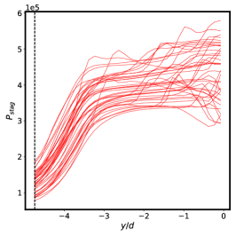
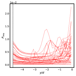
Five output observables are studied: stagnation pressure , root-mean-square (rms) static pressure , Mach number , turbulent kinetic energy TKE, and scalar dissipation rate . Examples of profiles for these observables across the wall-normal direction , at fixed streamwise direction , and averaged over time are shown in Fig. 6 for 2D under various parameter settings. In these plots, each red line is the profile of an independent simulation. The left side represents the lower wall of the chamber, with the dotted vertical line depicting the location of the wall; the right side represents the symmetry line of the chamber center. Effects of the boundary layer can be clearly seen through , , and .
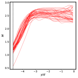
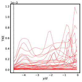
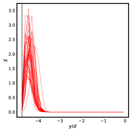
Our QOIs are the mean statistics of these five variables across and at fixed ; all QOIs are also time-averaged.666The variation due to time averaging depends on the location of averaging window (i.e., whether steady-state is reached), the inherent variation of the QOI, and the number of samples used for averaging. We perform the averaging over a window after transient behavior has sufficiently subsided, and detailed investigations on select runs indicate the overall time averaging variations is negligible compared to the variation of QOIs over the parameter space. We thus do not include them in the numerical results presented. Results for 3D simulations are taken at the centerline of the spanwise direction. Sample allocation across different models is calculated using MLMF MC, which minimizes the aggregate variance of MC estimators that correspond to each of the five QOIs. The number of runs for each model can be found in Table 2, where the desired general trend of fewer expensive simulations and more inexpensive simulations is evident (note that while 3D runs are not used in the PCE constructions above, they are still part of the MLMF MC allocation algorithm).
| 2D | 3D | |
|---|---|---|
| (coarse grid) | 1939 | 46 |
| (fine grid) | 79 | 11 |
The PCEs in Eqn. 36 and 37 are built for each QOI separately, using all available samples. GPSR is used to find a sparse PCE for each term, which are then combined together before a final relative thresholding (i.e., with respect to the coefficient of largest magnitude in that expansion) of is applied. For PCEs with total-order of degree 3, GPSR is able to downselect from a full set of 2925 basis terms to 187, 1336, 1676, 663, 2302 for the five QOIs in ML, and 200, 96, 308, 51, 352 in MF. The larger number of terms in ML is due to fewer available samples and a low signal-to-noise ratio for the difference between fine and coarse grid results.
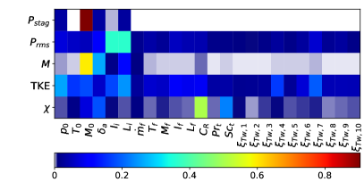
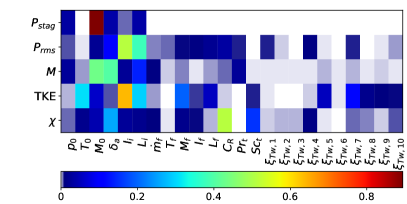
The total effect sensitivity indices are plotted in Fig. 7 for the ML and MF expansions. The rows depict the five QOIs (only the variable names are displayed in the figures, with the QOIs being these variables averaged over time and , and at ) and the columns correspond to the 24 input parameters. denotes the th KLE term for the wall temperature random field. Red spectrum indicates high sensitivity, and blue indicates low sensitivity (with grey-white being near-zero sensitivity). Sensitivity is relative within each QOI, thus one should not compare their values across different rows. Since the overall QOIs represented by the two expansions correspond to different fidelity and grid resolutions, one should not expect identical results (even under infinite samples), although it is reasonable to observe similar qualitative behavior. For both expansions, the most sensitive inputs tend to be those related to inflow conditions—, , , and have high sensitivity for one or more of the five QOIs. and also appear to be influential for the mean TKE, while is quite important for the mean scalar dissipation rate . Parameters corresponding to the wall temperature KLE have small contributions for most QOIs with all ten modes contributing under 5% variance. Exceptions are observed for mean receiving 25% in the ML expansion, and mean TKE receiving 67% and 21% in the ML and MF expansions, respectively. Overall, these observations are consistent with our physical intuition: since the current jet-in-crossflow test problem does not involve combustion, one would expect the bulk inflow conditions to dominate the impact on the QOI behavior. In future work involving the full HDCR geometry with combustion enabled, we expect to reveal different sensitivity trends under new interactions that would be otherwise nonintuitive and non-obvious.
5.2 Model error
We demonstrate the embedded representation of model error via two examples. The first involves 3D LES on a grid with resolution . The high-fidelity model uses a dynamic treatment of Smagorinsky turbulent characterization, where the Smagorinsky constant and turbulent Prandtl and Schmidt numbers are calculated locally at every grid point. The low-fidelity model employs a static treatment, where those parameters are fixed globally across the entire grid by the user. The static version provides about 30% saving of computational time. The second example calibrates a low-fidelity 2D model from evaluations of high-fidelity 3D simulations, and both models are simulated on the grid with the static Smagorinsky treatment. Even on this coarse grid, a 2D run requires two orders of magnitude less computational time compared to its 3D counterpart, and finer meshes would provide even greater cost savings. This is thus a realistic situation with strong tradeoff between accuracy and cost. In both cases, we would like to quantify the uncertainty due to model error when the less expensive low-fidelity model is used.
5.2.1 Static versus dynamic Smagorinsky
For the static model, we augment the modified Smagorinsky constant with an additive model error representation. It is endowed with a uniform prior , which is selected based on existing literature and preliminary simulation tests. The turbulent Prandtl and Schmidt numbers ( and ) are both fixed at a nominal value of . The calibration data are chosen to be the discretized profile of TKE along , and at fixed and spanwise centerline, for a total of 31 nodes. All QOIs, for both calibration and prediction, are time-averaged.777Similar to Footnote 6 in the GSA part, investigations on select cases indicate that variation due to time averaging is negligible compared to uncertainty contributions from model error and parameter posterior. We thus do not include them in the numerical results presented. Other choices of calibration QOIs are certainly possible, and ideally we would calibrate using the same QOIs for which we are interested in making predictions. We choose TKE here for demonstration. An interesting topic of future research is when calibration data are not available for predictive QOIs. Optimal experimental design methods can then be used to help choose from the available calibration QOIs those that are most useful for the predictive QOIs.
We set the additive term (from Eqn. 28) to be first-order Legendre-Uniform PCE in , i.e., model error representation is embedded in . The low-fidelity model surrogate, represented as a third-order Legendre polynomial, is built via regression using training samples, i.e., evaluations of the low-fidelity model at different values. The PCEs used for the likelihood and posterior predictive are third-order Legendre-Uniform, and integration over is performed using the 4-point Gaussian quadrature rule in each dimension. MCMC is run for samples, with 50% burn-in and thinning of every 100 samples to improve mixing.
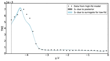
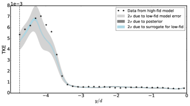
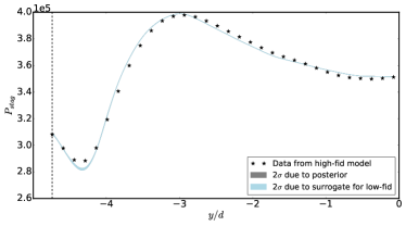
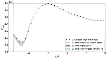
Figure 8 depicts the static Smagorinsky model posterior predictive distributions for the profiles of TKE and . The TKE profile constitutes the data set used for calibration, while the profile is extrapolatory. The left column displays classical Bayesian inference results, while the right column contains results with model error representation. The black dots are the true high-fidelity evaluations, and the light grey, dark grey, and blue bands represent standard deviations due to model error, posterior, and low-fidelity surrogate uncertainty, respectively, as broken down in Eqn. 35. In this case, the data set is overall quite informative, leading to very narrow posterior distributions (dark grey band) in all figures. The classical inference results in the left column lead us to be overconfident in predictive results that do not match well with the high-fidelity model in many regions. The strength of the model error representation is evident in the right column, as the light grey bands allow much better capturing of the model-to-model discrepancy, and present a better indication of our loss in model accuracy. In this example, the model error is characterized well for the extrapolatory QOIs ( profile, bottom-right figure). This may not always be the case, since the extrapolation of to QOIs outside those used for calibration may be inadequate, and there may be differences between high- and low-fidelity models that cannot be captured solely from parameter embedding. We will illustrate these challenges and limitations in the next example. Finally, we emphasize that all realizations generated from the posterior predictive distributions under this framework automatically satisfy the governing equations of the low-fidelity model.
5.2.2 2D versus 3D
In the second example, we calibrate a 2D model using data from 3D simulations. The parameters for the 2D model are endowed with uniform priors (see Table 3 for their definitions and prior ranges). Note that, for this example, we target the inverse Prandtl and Schmidt numbers instead of the non-inverted version used in the GSA cases. The 3D calibration data are generated at a fixed condition of . The calibration data are chosen to be the discretized profile of scalar dissipation rate along , at fixed and spanwise centerline, for a total of 31 nodes.
We embed the model error representation in and , allowing to be first-order Legendre-Uniform PCE for these two parameters only, while all other parameters are treated in the classical Bayesian inference sense (i.e., no embedding). A triangular structure is enforced for the multivariate expansion of Eqn. 26, which becomes
| (42) |
in accordance to the notation in Eqn. 9, and where we have substituted the first-order Legendre-Uniform polynomial basis . Priors with positive support are prescribed for and , which then guarantee a unique distribution for each realization of the triple . The decision of where to embed is guided by an initial GSA performed on the calibration QOIs: the profile. This is accomplished by using the low-fidelity surrogate Eqn. 28 to estimate the total sensitivity indices via the methodology in Eqn. 3 for each of the spatially-discretized grid points. Illustrated in Fig. 9, while sensitivity varies over , the overall most sensitive parameters, especially near the bottom wall (left side of the plot) where values are far from zero (e.g., see Fig. 10 first row), are and . It is thus reasonable to expect the model error embedding to be most effective when applied on these two parameters. Indeed, in separate studies (results omitted), embedding in other parameters displayed less effective capturing of QOI discrepancy between the two models. The low-fidelity model surrogate is built using third-order Legendre polynomial from 500 regression samples. The PCEs used for the likelihood and posterior predictive are third-order Legendre-Uniform, and integration over is performed using the 4-point Gaussian quadrature rule in each dimension. MCMC is run for samples, with 50% burn-in and thinning of every 100 samples to improve mixing.
| Parameter | Range | Description |
|---|---|---|
| [0.005, 0.08] | Modified Smagorinsky constant | |
| [0.25, 2.0] | Inverse turbulent Prandtl number | |
| [0.25, 2.0] | Inverse turbulent Schmidt number | |
| [0.025, 0.075] | Inlet turbulence intensity magnitude in horizontal direction | |
| [0.5, 1.0] | Inlet turbulence intensity vertical to horizontal ratio | |
| [0.0, 8.0] mm | Inlet turbulence length scale |
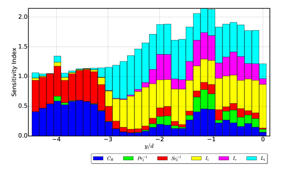
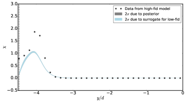
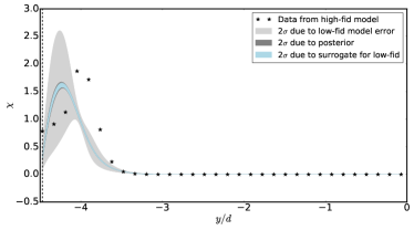
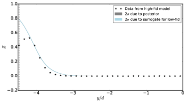
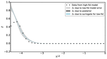
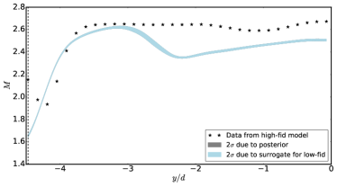
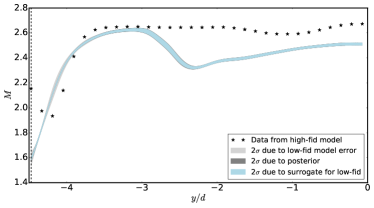
Figure 10 depicts the 2D model posterior predictive distributions for the profiles of scalar dissipation rate , mixture fraction , and Mach number . The scalar dissipation rate profile constitutes data used for calibration, while other QOIs are extrapolatory. Overall, we see that the light grey band covers the model-to-model discrepancy reasonably well for , but there are small regions where the high-fidelity data are uncovered (e.g., around ). For , we observe reasonable performance to the right of the second grid point; and for , the light grey band is nearly non-existent (and thus has poor discrepancy coverage).
There are two important factors that explain these observed limitations. The first reason is a challenge for all model error approaches and not specific to the embedded representation: the extrapolation of for use on QOIs outside the calibration set (as described in Eqn. 24, e.g., extrapolated from to and profiles in this example) may be inadequate and lead to poor coverage of model-to-model discrepancy from the uncertainty bands. This is one contributing factor for the mismatched regions of the mid-right and bottom-right plots in Fig. 10. However, even in some regions of the calibration QOIs (top-right plot), the light grey band does not extend to cover the high-fidelity data points. This brings us to our second reason that also demonstrates the limitation of the embedded representation: the model error bands can only be as wide as the QOI ranges allowed by the parameter variation (within the bounds of the uniform prior of in this case). This constraint presents a difficulty when the QOI outputs from the low- and high-fidelity models are simply too different, and cannot be compensated in the low-fidelity model by varying its parameter values. In our application, the 2D model is indeed physically very different from the 3D in many aspects, and is unable to capture many detailed physical features. (In contrast, the previous study of static and dynamic Smagorinsky models presented much closer QOI behaviors.) For instance, a bow shock structure forms in the 3D setup, and would not be portrayed in 2D. This difference can also change the locations where the shocks reflect, thus yielding very different “slice” profiles. Furthermore, fuel injectors in 3D are circular (not slotted), and not equivalent to a simple extrusion of the 2D geometry. The shock strength is thus expected to be weaker in the 3D model due to the relatively smaller area of fuel injection. These insights are supported by the profile plots, where the shocks are suggested by the dips in the profiles. Additional studies (results omitted) indeed confirm that the posterior predictive bands from the right column of Fig. 10 are similar to those of the prior predictive, i.e., the widest allowable by the ranges in Table 3. This lowered flexibility of capturing model discrepancy is the price for requiring the governing equations to be respected in the predictive results. At the same time, it also inspires interesting future work directions. To begin with, we would like to explore other forms of embedding that could be more advantageous, both in terms of selection of as well as advanced structuring of . Another possibility is to construct a hierarchy of intermediate models that offers a smoother transition between the high- and low-fidelity models, which also complements the multi-model theme in Sec. 3.1. We plan to develop these techniques as we proceed to the full HDCR domain with combustion enabled.
6 Conclusions
The development of scramjet engines is an important area of research for advancing hypersonic and orbital flights. Progress towards optimal engine designs requires accurate flow simulations together with uncertainty quantification (UQ). However, performing UQ for scramjet simulations is extremely challenging due to the large number of uncertain parameters involved and the high computational cost of performing flow simulations. This paper addressed these difficulties by developing practical UQ algorithms and computational methods, and deploying them to a jet-in-crossflow problem in a simplified HIFiRE Direct Connect Rig (HDCR) scramjet combustor. To start, a jet-in-crossflow test problem was formulated for the primary injector section subdomain of the HDCR, with a focus on the interaction between fuel jet and the supersonic crossflow without combustion. Large-eddy simulation (LES) was used to model the turbulent flow physics, and the fully coupled system of conservation laws was solved by the RAPTOR code.
Global sensitivity analysis (GSA) was conducted to identify the most influential uncertain input parameters, providing important information to help reduce the system’s stochastic dimension. GSA was efficiently performed by leveraging multilevel and multifidelity frameworks that combined evaluations from different models, polynomial chaos expansion (PCE) surrogates that provided a convenient form for calculating sensitivity indices, and compressed sensing that discovered sparse PCE forms from limited simulation data. Through GSA, six important input parameters were established from an initial set of 24.
A framework was then introduced for quantifying and propagating uncertainty due to model error. This technique involved embedding a correction term directly in the parameters of the low-fidelity model, thus guaranteeing the predictions to maintain satisfaction of the underlying governing equations and physical laws. The correction term was represented in a stochastic and Bayesian manner, and calibrated using Markov chain Monte Carlo. Both the strengths and weaknesses of this approach were highlighted via applications of static-versus-dynamic Smagorinsky turbulent treatments as well as 2D-versus-3D geometries.
The logical next step is to extend these UQ techniques to the full HDCR configuration (Fig. 2(a)). Additional challenges are expected to emerge, both for LES involving a more complex cavity geometry with combustion, and UQ that will face even higher dimensional settings, increasingly expensive model evaluations, and fewer data points. Additional numerical developments will be essential to overcome these obstacles, with fruitful avenues of exploration that include adaptive and robust quadrature methods, Bayesian model selection, and efficient MCMC for model calibration.
Acknowledgments
Support for this research was provided by the Defense Advanced Research Projects Agency (DARPA) program on Enabling Quantification of Uncertainty in Physical Systems (EQUiPS). Sandia National Laboratories is a multimission laboratory managed and operated by National Technology and Engineering Solutions of Sandia, LLC., a wholly owned subsidiary of Honeywell International, Inc., for the U.S. Department of Energy’s National Nuclear Security Administration under contract DE-NA-0003525.
References
- [1] V. Barthelmann, E. Novak, and K. Ritter, High dimensional polynomial interpolation on sparse grids, Advances in Computational Mathematics, 12 (2000), pp. 273–288, https://doi.org/10.1023/A:1018977404843.
- [2] E. J. Candès, J. Romberg, and T. Tao, Robust Uncertainty Principles: Exact Signal Reconstruction From Highly Incomplete Frequency Information, IEEE Transactions on Information Theory, 52 (2006), pp. 489–509, https://doi.org/10.1109/TIT.2005.862083.
- [3] R. Christensen, Plane Answers to Complex Questions: The Theory of Linear Models, Springer-Verlag New York, New York, NY, 4th ed., 2011.
- [4] P. G. Constantine, M. Emory, J. Larsson, and G. Iaccarino, Exploiting active subspaces to quantify uncertainty in the numerical simulation of the HyShot II scramjet, Journal of Computational Physics, 302 (2015), pp. 1–20, https://doi.org/10.1016/j.jcp.2015.09.001.
- [5] D. J. Dolvin, Hypersonic International Flight Research and Experimentation (HIFiRE), in 15th AIAA International Space Planes and Hypersonic Systems and Technologies Conference, no. 2008-2581, Dayton, OH, 2008, https://doi.org/10.2514/6.2008-2581.
- [6] D. J. Dolvin, Hypersonic International Flight Research and Experimentation, in 16th AIAA/DLR/DGLR International Space Planes and Hypersonic Systems and Technologies Conference, no. 2009-7228, Bremen, Germany, 2009, https://doi.org/10.2514/6.2009-7228.
- [7] D. L. Donoho, Compressed sensing, IEEE Transactions on Information Theory, 52 (2006), pp. 1289–1306, https://doi.org/10.1109/Tit.2006.871582.
- [8] D. L. Donoho, For Most Large Underdetermined Systems of Linear Equations the Minimal -norm Solution Is Also the Sparsest Solution, Communications on Pure and Applied Mathematics, 59 (2006), pp. 797–829, https://doi.org/10.1002/cpa.20132.
- [9] M. S. Eldred, L. W. T. Ng, M. F. Barone, and S. P. Domino, Multifidelity Uncertainty Quantification Using Spectral Stochastic Discrepancy Models, in Handbook of Uncertainty Quantification, Springer International Publishing, Cham, 2015, pp. 1–45, https://doi.org/10.1007/978-3-319-11259-6_25-1.
- [10] O. G. Ernst, A. Mugler, H.-J. Starkloff, and E. Ullmann, On the convergence of generalized polynomial chaos expansions, ESAIM: Mathematical Modelling and Numerical Analysis, 46 (2012), pp. 317–339, https://doi.org/10.1051/m2an/2011045.
- [11] N. Fajraoui, S. Marelli, and B. Sudret, On Optimal Experimental Designs for Sparse Polynomial Chaos Expansions, Tech. Report RSUQ-2017-001, ETH Zurich, 2017.
- [12] P. G. Ferlemann, Forebody and Inlet Design for the HIFiRE 2 Flight Test, in JANNAF Airbreathing Propulsion Subcommittee Meeting, Boston, MA, 2008.
- [13] M. A. T. Figueiredo, R. D. Nowak, and S. J. Wright, Gradient Projection for Sparse Reconstruction: Application to Compressed Sensing and Other Inverse Problems, IEEE Journal of Selected Topics in Signal Processing, 1 (2007), pp. 586–597, https://doi.org/10.1109/JSTSP.2007.910281.
- [14] M. A. T. Figueiredo, R. D. Nowak, and S. J. Wright, GPSR: Gradient Projection for Sparse Reconstruction. http://www.lx.it.pt/~mtf/GPSR/, 2009. (accessed 2017-05-03).
- [15] G. Geraci, M. S. Eldred, and G. Iaccarino, A multifidelity control variate approach for the multilevel Monte Carlo technique, Tech. Report Center for Turbulence Research Annual Research Briefs, Stanford University, 2015.
- [16] G. Geraci, M. S. Eldred, and G. Iaccarino, A multifidelity multilevel Monte Carlo method for uncertainty propagation in aerospace applications, in 19th AIAA Non-Deterministic Approaches Conference, no. 2017-1951, Grapevine, TX, 2017, https://doi.org/10.2514/6.2017-1951.
- [17] T. Gerstner and M. Griebel, Numerical integration using sparse grids, Numerical Algorithms, 18 (1998), pp. 209–232, https://doi.org/10.1023/A:1019129717644.
- [18] T. Gerstner and M. Griebel, Dimension-Adaptive Tensor-Product Quadrature, Computing, 71 (2003), pp. 65–87, https://doi.org/10.1007/s00607-003-0015-5.
- [19] R. G. Ghanem and P. D. Spanos, Stochastic Finite Elements: A Spectral Approach, Springer New York, New York, NY, 1st ed., 1991.
- [20] M. B. Giles, Multilevel Monte Carlo Path Simulation, Operations Research, 56 (2008), pp. 607–617, https://doi.org/10.1287/opre.1070.0496.
- [21] W. R. Gilks, S. Richardson, and D. J. Spiegelhalter, Markov Chain Monte Carlo in Practice, Chapman & Hall, New York, NY, 1996.
- [22] M. R. Gruber, P. Ferlemann, and K. McDaniel, HIFiRE Flight 2 Flowpath Design Update, Tech. Report AFRL-RZ-WP-TP-2010-2247, AFRL, 2009.
- [23] M. R. Gruber, K. Jackson, and J. Liu, Hydrocarbon-Fueled Scramjet Combustor Flowpath Development for Mach 6-8 HIFiRE Flight Experiments, Tech. Report AFRL-RZ-WP-TP-2010-2243, AFRL, 2008.
- [24] H. Haario, E. Saksman, and J. Tamminen, An adaptive Metropolis algorithm, Bernoulli, 7 (2001), pp. 223–242.
- [25] J. Hampton and A. Doostan, Compressive sampling of polynomial chaos expansions: Convergence analysis and sampling strategies, Journal of Computational Physics, 280 (2015), pp. 363–386, https://doi.org/10.1016/j.jcp.2014.09.019.
- [26] N. E. Hass, K. F. Cabell, and A. M. Storch, HIFiRE Direct-Connect Rig (HDCR) Phase I Ground Test Results from the NASA Langley Arc-Heated Scramjet Test Facility, Tech. Report LF99-8888, NASA, 2010.
- [27] T. Hastie, R. Tibshirani, and J. Friedman, The Elements of Statistical Learning, Springer, New York, NY, 2nd ed., 2009.
- [28] X. Huan, C. Safta, K. Sargsyan, Z. P. Vane, G. Lacaze, J. C. Oefelein, and H. N. Najm, Compressive Sensing with Cross-Validation and Stop-Sampling for Sparse Polynomial Chaos Expansions, arXiv:1707.09334, (2017), https://arxiv.org/abs/1707.09334.
- [29] K. R. Jackson, M. R. Gruber, and T. F. Barhorst, The HIFiRE Flight 2 Experiment: An Overview and Status Update, in 45th AIAA/ASME/SAE/ASEE Joint Propulsion Conference & Exhibit, no. 2009-5029, Denver, CO, 2009, https://doi.org/10.2514/6.2009-5029.
- [30] K. R. Jackson, M. R. Gruber, and S. Buccellato, HIFiRE Flight 2 Overview and Status Uptate 2011, in 17th AIAA International Space Planes and Hypersonic Systems and Technologies Conference, no. 2011-2202, San Francisco, CA, 2011, https://doi.org/10.2514/6.2011-2202.
- [31] J. D. Jakeman, M. S. Eldred, and K. Sargsyan, Enhancing -minimization estimates of polynomial chaos expansions using basis selection, Journal of Computational Physics, 289 (2015), pp. 18–34, https://doi.org/10.1016/j.jcp.2015.02.025.
- [32] M. J. W. Jansen, Analysis of variance designs for model output, Computer Physics Communications, 117 (1999), pp. 35–43, https://doi.org/10.1016/S0010-4655(98)00154-4.
- [33] M. C. Kennedy and A. O’Hagan, Bayesian calibration of computer models, Journal of the Royal Statistical Society: Series B (Statistical Methodology), 63 (2001), pp. 425–464, https://doi.org/10.1111/1467-9868.00294.
- [34] M. Khalil, G. Lacaze, J. C. Oefelein, and H. N. Najm, Uncertainty quantification in LES of a turbulent bluff-body stabilized flame, Proceedings of the Combustion Institute, 35 (2015), pp. 1147–1156, https://doi.org/10.1016/j.proci.2014.05.030.
- [35] G. Lacaze, A. Misdariis, A. Ruiz, and J. C. Oefelein, Analysis of high-pressure Diesel fuel injection processes using LES with real-fluid thermodynamics and transport, Proceedings of the Combustion Institute, 35 (2015), pp. 1603–1611, https://doi.org/10.1016/j.proci.2014.06.072.
- [36] G. Lacaze, Z. P. Vane, and J. C. Oefelein, Large Eddy Simulation of the HIFiRE Direct Connect Rig Scramjet Combustor, in 55th AIAA Aerospace Sciences Meeting and Exhibit, no. 2017-0142, Grapevine, TX, 2017, https://doi.org/10.2514/6.2017-0142.
- [37] O. P. Le Maître and O. M. Knio, Spectral Methods for Uncertainty Quantification: with Applications to Computational Fluid Dynamics, Springer Netherlands, Houten, Netherlands, 2010.
- [38] H. N. Najm, Uncertainty Quantification and Polynomial Chaos Techniques in Computational Fluid Dynamics, Annual Review of Fluid Mechanics, 41 (2009), pp. 35–52, https://doi.org/10.1146/annurev.fluid.010908.165248.
- [39] B. K. Natarajan, Sparse Approximate Solutions to Linear Systems, SIAM Journal on Computing, 24 (1995), pp. 227–234, https://doi.org/10.1137/S0097539792240406.
- [40] L. W. T. Ng and M. Eldred, Multifidelity Uncertainty Quantification Using Non-Intrusive Polynomial Chaos and Stochastic Collocation, in 53rd AIAA/ASME/ASCE/AHS/ASC Structures, Structural Dynamics and Materials Conference, no. 2012-1852, Honolulu, Hawaii, 2012, https://doi.org/doi:10.2514/6.2012-1852.
- [41] J. C. Oefelein, Simulation and Analysis of Turbulent Multiphase Combustion Processes at High Pressures, PhD thesis, The Pennsylvania State University, University Park, Pennsylvania, May 1997.
- [42] J. C. Oefelein, Large eddy simulation of turbulent combustion processes in propulsion and power systems, Progress in Aerospace Sciences, 42 (2006), pp. 2–37, https://doi.org/10.1016/j.paerosci.2006.02.001.
- [43] J. C. Oefelein, Large Eddy Simulation of Complex Thermophysics in Advanced Propulsion and Power Systems, in Proceedings of the 8th U.S. National Combustion Meeting, Park City, UT, 2013.
- [44] J. C. Oefelein, R. Dahms, and G. Lacaze, Detailed Modeling and Simulation of High-Pressure Fuel Injection Processes in Diesel Engines, SAE International Journal of Engines, 5 (2012), pp. 1411–1419, https://doi.org/10.4271/2012-01-1258.
- [45] J. C. Oefelein, G. Lacaze, R. Dahms, A. Ruiz, and A. Misdariis, Effects of Real-Fluid Thermodynamics on High-Pressure Fuel Injection Processes, SAE International Journal of Engines J. Engines, 7 (2014), pp. 1125–1136, https://doi.org/10.4271/2014-01-1429.
- [46] J. C. Oefelein, V. Sankaran, and T. G. Drozda, Large eddy simulation of swirling particle-laden flow in a model axisymmetric combustor, Proceedings of the Combustion Institute, 31 (2007), pp. 2291–2299, https://doi.org/10.1016/j.proci.2006.08.017.
- [47] J. C. Oefelein, R. W. Schefer, and R. S. Barlow, Toward Validation of Large Eddy Simulation for Turbulent Combustion, AIAA Journal, 44 (2006), pp. 418–433, https://doi.org/10.2514/1.16425.
- [48] T. A. Oliver, G. Terejanu, C. S. Simmons, and R. D. Moser, Validating predictions of unobserved quantities, Computer Methods in Applied Mechanics and Engineering, 283 (2015), pp. 1310–1335, https://doi.org/10.1016/j.cma.2014.08.023.
- [49] B. Peherstorfer, K. Willcox, and M. Gunzburger, Survey of multifidelity methods in uncertainty propagation, inference , and optimization, Tech. Report ACDL technical Report TR16-1, Massachusetts Institute of Technology, 2016.
- [50] J. Peng, J. Hampton, and A. Doostan, A weighted -minimization approach for sparse polynomial chaos expansions, Journal of Computational Physics, 267 (2014), pp. 92–111, https://doi.org/10.1016/j.jcp.2014.02.024.
- [51] H. Rauhut and R. Ward, Sparse Legendre expansions via -minimization, Journal of Approximation Theory, 164 (2012), pp. 517–533, https://doi.org/10.1016/j.jat.2012.01.008.
- [52] G. O. Roberts, General state space Markov chains and MCMC algorithms, Probability Surveys, 1 (2004), pp. 20–71, https://doi.org/10.1214/154957804100000024.
- [53] A. Saltelli, Making best use of model evaluations to compute sensitivity indices, Computer Physics Communications, 145 (2002), pp. 280–297, https://doi.org/10.1016/S0010-4655(02)00280-1.
- [54] A. Saltelli, P. Annoni, I. Azzini, F. Campolongo, M. Ratto, and S. Tarantola, Variance based sensitivity analysis of model output. Design and estimator for the total sensitivity index, Computer Physics Communications, 181 (2010), pp. 259–270, https://doi.org/10.1016/j.cpc.2009.09.018.
- [55] A. Saltelli, M. Ratto, T. Andres, F. Campolongo, J. Cariboni, D. Gatelli, M. Saisana, and S. Tarantola, Global Sensitivity Analysis: The Primer, John Wiley & Sons, Chichester, United Kingdom, 2008.
- [56] A. Saltelli, S. Tarantola, F. Campolongo, and M. Ratto, Sensitivity Analysis in Practice: A Guide to Assessing Scientific Models, John Wiley & Sons, Chichester, United Kingdom, 2004.
- [57] A. Saltelli, S. Tarantola, and K. P.-S. Chan, A Quantitative Model-Independent Method for Global Sensitivity Analysis of Model Output, Technometrics, 41 (1999), pp. 39–56, https://doi.org/10.1080/00401706.1999.10485594.
- [58] K. Sargsyan, H. N. Najm, and R. G. Ghanem, On the Statistical Calibration of Physical Models, International Journal of Chemical Kinetics, 47 (2015), pp. 246–276, https://doi.org/10.1002/kin.20906.
- [59] K. Sargsyan, C. Safta, H. N. Najm, B. J. Debusschere, D. Ricciuto, and P. Thornton, Dimensionality Reduction for Complex Models via Bayesian Compressive Sensing, International Journal for Uncertainty Quantification, 4 (2014), pp. 63–93, https://doi.org/10.1615/Int.J.UncertaintyQuantification.2013006821.
- [60] J. D. Schmisseur, Hypersonics into the 21st century: A perspective on AFOSR-sponsored research in aerothermodynamics, Progress in Aerospace Sciences, 72 (2015), pp. 3–16, https://doi.org/10.1016/j.paerosci.2014.09.009.
- [61] I. M. Sobol, On sensitivity estimation for nonlinear mathematical models, Matematicheskoe Modelirovanie, 2 (1990), pp. 112–118.
- [62] I. M. Sobol, Theorems and examples on high dimensional model representation, Reliability Engineering & System Safety, 79 (2003), pp. 187–193, https://doi.org/10.1016/S0951-8320(02)00229-6.
- [63] A. M. Storch, M. Bynum, J. Liu, and M. Gruber, Combustor Operability and Performance Verification for HIFiRE Flight 2, in 17th AIAA International Space Planes and Hypersonic Systems and Technologies Conference, no. 2011-2249, San Francisco, CA, 2011, https://doi.org/10.2514/6.2011-2249.
- [64] T. C. Williams, R. W. Schefer, J. C. Oefelein, and C. R. Shaddix, Idealized gas turbine combustor for performance research and validation of large eddy simulations, Review of Scientific Instruments, 78 (2007), pp. 1–9, https://doi.org/10.1063/1.2712936.
- [65] J. Witteveen, K. Duraisamy, and G. Iaccarino, Uncertainty Quantification and Error Estimation in Scramjet Simulation, in 17th AIAA International Space Planes and Hypersonic Systems and Technologies Conference, no. 2011-2283, 2011, https://doi.org/10.2514/6.2011-2283.
- [66] D. Xiu, Fast Numerical Methods for Stochastic Computations: A Review, Communications in Computational Physics, 5 (2009), pp. 242–272.
- [67] D. Xiu and G. E. Karniadakis, The Wiener-Askey Polynomial Chaos for Stochastic Differential Equations, SIAM Journal on Scientific Computing, 24 (2002), pp. 619–644, https://doi.org/10.1137/S1064827501387826.