Notes on Melonic $O(N)^{q-1}$ Tensor Models

Abstract

It has recently been demonstrated that the large N limit of a model of fermions charged under the global/gauge symmetry group $O(N)^{q-1}$ agrees with the large $N$ limit of the SYK model. In these notes we investigate aspects of the dynamics of the $O(N)^{q-1}$ theories that differ from their SYK counterparts. We argue that the spectrum of fluctuations about the finite temperature saddle point in these theories has $(q-1)\frac{N^{2}}{2}$ new light modes in addition to the light Schwarzian mode that exists even in the SYK model, suggesting that the bulk dual description of theories differ significantly if they both exist. We also study the thermal partition function of a mass deformed version of the SYK model. At large mass we show that the effective entropy of this theory grows with energy like $E\ln E$ (i.e. faster than Hagedorn) up to energies of order $N^{2}$. The canonical partition function of the model displays a deconfinement or Hawking Page type phase transition at temperatures of order $1/\ln N$. We derive these results in the large mass limit but argue that they are qualitatively robust to small corrections in $J/m$.

1 Introduction

It has recently been demonstrated that the dynamically rich Sachdev-Ye-Kitaev model - a quantum mechanical model of fermions interacting with random potentials - is solvable at large $N$ Sachdev:2010um ; kitaev-talk ; Maldacena:2016hyu . This model is interesting partly because its thermal properties have several features in common with those of black holes. The SYK model self equilibrates over a time scale of order the inverse temperature and has a Lyapunov index that saturates the chaos bound Maldacena:2016hyu ; kitaev-talk . Moreover the long time behaviour of this model at finite temperature is governed by an effective action that has been reinterpreted as a particular theory of gravity expanded about $AdS_{2}$ background solution Sachdev:2010um ; Almheiri:2014cka ; Jensen:2016pah ; Maldacena:2016upp ; Mandal:2017thl ; Gross:2017hcz ; Forste:2017kwy ; Das:2017pif .

These facts have motivated the suggestion that the SYK model is the boundary dual of a highly curved bulk gravitational theory whose finite temperature behaviour is dominated by a black hole saddle point. If this suggestion turns out to be correct, the solvability of the SYK model at large $N$ - and its relative simplicity even at finite $N$- could allow one to probe old mysteries of black hole physics in a manner that is nonperturbative in $\frac{1}{N}$, the effective dual gravitational coupling (see e.g. Garcia-Garcia:2016mno ; Cotler:2016fpe ; Garcia-Garcia:2017pzl for recent progress).

There is, however, a potential fly in the ointment. While the SYK model - defined as a theory with random couplings - is an average over quantum systems, it is not a quantum system by itself. One cannot, for instance, associate the SYK model with a Hilbert space in any completely precise manner, or find a unitary operator that generates time evolution in this model. As several of the deepest puzzles of black hole physics concern conflicts with unitarity, this feature of the SYK model is a concern.

Of course any particular realisation of the couplings drawn from the SYK ensemble is a genuine quantum theory. It is plausible that several observables - like the partition function - have the same large $N$ limit when computed for any given typical member of the ensemble as they do for the SYK model defined by averaging over couplings Cotler:2016fpe ; Stanford:2017thb ; Belokurov:2017eit . It might thus seem that every typical realization of random couplings is an inequivalent consistent quantization of classical large $N$ SYK system. As the number of such quantizations is very large, this would be an embarrassment of riches. The potential issue here is that if we work with any given realization of the SYK model, it appears inconsistent to restrict attention to averaged observables for any finite $N$ no matter how large. On the other hand correlators of individual $\psi_{i}$ operators (as opposed to their averaged counterparts) presumably do not have a universal large $N$ limit (and so are not exactly solvable even at large $N$).

In order to address these concerns some authors have recently Witten:2016iux ; Klebanov:2016xxf ; Klebanov:2017nlk (based on earlier work Gurau:2009tw ; Gurau:2010ba ; Gurau:2011aq ; Gurau:2011xq ; Bonzom:2011zz ; Gurau:2011xp ) studied a related class of models. These models are ordinary quantum mechanical systems; in fact they describe the global or gauged quantum mechanics of a collection of fermions in 0+1 dimensions. In this paper we will focus our attention on the model

$$\begin{split}&S=\int dt\sum_{a=1}^{N_{F}}[{\bar{\psi}}_{a}D_{0}\psi_{a}-\left(g\ \psi_{a}^{q}+h.c.\right)],\\ &D_{0}=\partial_{0}+iA_{0}\ ,\ g=\frac{J}{N^{\frac{(q-1)(q-2)}{4}}},\\ \end{split}$$ (1)

that was first proposed - at least in the current context - in Klebanov:2016xxf . In (1) $\psi_{a}$ are a collection of complex gauged fermionic fields in $0+1$ dimensions that transform in the fundamental of each of the $q-1$ copies of $O(N)$. The index $a$ is a flavour index that runs from $1\ldots N_{F}$. . $J$ is a coupling constant with dimensions of mass and $\psi^{q}$ is a schematic for a $q$ vertex generalisation of a ‘tetrahedronal’ interaction term between $q$ copies of the fermionic fields, whose gauge index contraction structure is explained in detail in Witten:2016iux ; Klebanov:2016xxf and will be elaborated on below.

The tetrahedral structure of the interactionWitten:2016iux ; Klebanov:2016xxf is such that for any even number of fermions $q$ each fermion has $q-1$ indices each in a different $O(N)({\textrm{o}r}\,U(N))$. The indices among the $q$ fermions are contracted such that every fermion is index contracted with an index of the same gauge group on one of the remaining fermions. Moreover, given any - and every - 2 fermions have a single index (of some gauge group) contracted between them. For $q=4$ it is easy to check that these words define a unique contraction structure which may be viewed as a tetrahedral contraction among the 4 fermions each with $q-1=3$ indices(legs) with every fermion(point or vertex of the tetrahedron) connected to 3 different coloured legs. For $q\geq 6$ it is not clear that the words above define a unique contraction structure. In case the contraction structure is not unique, we pick one choice - for example the Round-Robin scheduling process to define our interaction Narayan:2017qtw ; Yoon:2017nig .

The connection between the quantum mechanical theories (1) and the SYK model itself is the following; it has been demonstrated (subject to certain caveats) that sum over Feynman graphs of the theory (1) coincides with the sum over Feynman graphs of the SYK model at at leading order at large $N$ (see Witten:2016iux for the argument in a very similar model), even though these two sums differ at finite values of $N$ (see e.g. the recent paper Dartois:2017xoe and references therein). It follows that the quantum mechanical models (1) are exactly as solvable as the SYK model at large $N$; moreover they also inherit much of the dynamical richness of the SYK model. In other words the models (1) are solvable at large $N$, are unitary and are potentially boundary duals of (highly curved) black hole physics.

Motivated by these considerations, in this note we study the effective theory that governs the long time dynamics of the model (1) at finite temperature. We focus attention on dynamical aspects of (1) that have no counterpart in the already well studied dynamics of the original SYK model.

In the rest of this introduction we will explain and describe our principal observations and results.

1.1 New light modes

The thermal behaviour of both the theory (1) and the original SYK model is determined by the path integral of these theories on a circle of circumference $\beta$.

It was demonstrated in kitaev-talk ; Maldacena:2016hyu that, in the case of the original SYK model, this path integral is dominated by a saddle point of an effective action whose fields are the two point function and self energy of the fermions. An extremization of this effective action determines both the fermionic two point function at finite temperature as well as the free energy of the system at leading order at large $N$.

In a similar manner, the thermal behaviour of the quantum mechanical systems (1) is dominated by a saddle point at large $N$. Under appropriate assumptions it may be shown that resultant effective action has the same minimum as that of the original SYK theory Witten:2016iux . . Specialising to the case $N_{F}=1$, the leading order fermionic two point function of the quantum mechanical system is given by

$$\langle{\bar{\psi}}^{a}(t)\psi_{b}(t^{\prime})\rangle=\delta^{a}_{b}G^{SYK}(t-t^{\prime}),$$ (2)

where $a$ and $b$ denote the (collection of) vector indices for the fermions and $G^{SYK}(t)$ is the thermal propagator of the original SYK model.

While the thermal behaviour of the model (1) is thus indistinguishable from that of the SYK model at leading order in the large $N$ limit, the dynamics of the quantum mechanical model (1) differs from that of the SYK model at subleading orders in $1/N$. The first correction to leading large $N$ thermal behaviour may be obtained by performing a one loop path integral over quadratic fluctuations around the saddle point. In the long time limit, correlators are dominated by the lightest fluctuations around the saddle point.

Recall that in the UV (i.e. as $\beta J\rightarrow 0$ ) the fermions of (1) have dimension zero. The term proportional to $\psi^{q}$ in (1) represents a dimension zero relevant deformation of this UV fixed point. The resultant RG flow ends in the deep IR in a conformal field theory in which the fermions have dimension $\frac{1}{q}$. kitaev-talk ; Maldacena:2016hyu . In this IR limit (relevant to thermodynamics when $\beta J\to\infty$) $\psi^{q}$ is marginal while the kinetic term in (1) is irrelevant kitaev-talk ; Maldacena:2016hyu . The fact that the kinetic term is irrelevant in the IR - and so can effectively be ignored in analysing the symmetries of (1) at large $\beta J$ - has important implications for the structure of light fluctuations about the thermal saddle point.

The first implication of the irrelevance of the kinetic term occurs already in the SYK model and was explored in detail in kitaev-talk ; Maldacena:2016hyu ; Maldacena:2016upp . The main point is that the action (1), with the kinetic term omitted, enjoys invariance under conformal diffeomorphisms (i.e. diffeomorphisms together with a Weyl transformation). However the saddle point solution for the Greens function $G^{\text{SYK}}(t)$ is not invariant under conformal diffeomorphisms. It follows immediately that the action of infinitesimal conformal diffeomorphisms on this solution generates zero modes in the extreme low energy limit.

At any finite temperature, no matter how small, the kinetic term in (1) cannot completely be ignored and conformal invariance is broken; the action of conformal diffeomorphisms on the SYK saddle point consequently produces anomalously light (rather than exactly zero) modes. The action for these modes was computed in kitaev-talk ; Maldacena:2016hyu ; Maldacena:2016upp and takes the form of the Schwarzian for the conformal diffeomorphisms.

A very similar line of reasoning leads to the conclusion that the model (1) has $(q-1)\frac{N^{2}}{2}$ additional light modes in the large $\beta J$ limit, as we now explain. Let us continue to work in the gauge $A_{0}=0$. In this gauge the action (1) is obviously invariant under the global rotations $\psi\rightarrow V\psi$, ${\bar{\psi}}\rightarrow{\bar{\psi}}V^{\dagger}$ where $V$ is an arbitrary time independent $O(N)^{q-1}$ rotation. In the global model (1) the rotation by $V$ is the action of a global symmetry. In gauged model on the other hand, these rotations are part of the gauge group and do not generate global symmetries of our model; the Gauss law in the theory ensures that all physical states are uncharged under this symmetry.

Let us now consider the transformation $\psi\rightarrow V(t)\psi$ together with ${\bar{\psi}}\rightarrow{\bar{\psi}}V(t)^{\dagger}$ where $V(t)$ is an arbitrary time dependent $O(N)^{q-1}$ rotation. In the case of the gauged models, this transformation is not accompanied by a change in $A_{0}$ ($A_{0}=const$ throughout) so the rotation is not a gauge transformation.

At finite $\beta J$ the rotation by a time dependent $V(t)$ is not a symmetry of the action (1) in either the global or the gauged theory as the kinetic term in (1) is not left invariant by this transformation. As we have explained above, however, the kinetic term is irrelevant in the low temperature limit $\beta J\to\infty$. It follows that the time dependent transformation is an effective symmetry of dynamics this strict low temperature limit.

However the saddle point solution (2) is clearly not invariant under the time dependent rotations by $V(t)$. It follows that, as in the discussion for conformal diffeomorphisms above, the action of $V(t)$ on (2) generates exact zero modes in the strict limit $\beta J\to\infty$ and anomalously light modes at any finite $\beta J$. We emphasise that this discussion applies both to the global model where $O(N)^{q-1}$ is a global symmetry, and the gauged model where it is not.

In section 2.2 below we argue that the dynamics of our new light modes is governed by the effective sigma model on the group manifold

$$S=-\mathcal{A}\ \frac{N^{q-2}}{|J|}\int dt\ \sum_{l=1}^{q-1}\ Tr\ \left[\left(V_{l}^{-1}(t)\ \frac{\partial}{\partial t}V_{l}(t)\right)^{2}\right],$$ (3)

where $V_{l}(t)$ is an arbitrary element of the group $O(N)$ and $\mathcal{A}$ is a number of order unity that we have not been able to determine.

The formula (3) has appeared before in a closely related context. The authors of Sachdev:2017mar (see also Stanford:2017thb ) studied the a complex version of the SYK model. Their model had an exact $U(1)$ symmetry at all energies, which - using the arguments presented in the previous paragraphs - was approximately enhanced to a local $U(1)$ symmetry at low energies. The authors of Sachdev:2017mar argued the long distance dynamics of the new light modes is governed by a sigma model on the group manifold $U(1)$. Given these results, the appearance of a low energy sigma model in the large $\beta J$ finite temperature dynamics of the theory (1) seems natural.

We would, however, like to emphasise two qualitative differences between the sigma model (3) and the model that appeared in Sachdev:2017mar . First (3) is a sigma model for a group $O(N)^{q-1}$ whose dimensionality goes to infinity in the large $N$ limit, $N\to\infty$. Second that we find the new light modes of the action even of the gauged model (1) even though $O(N)^{q-1}$ is not a global symmetry of this theory.

The new modes governed by (3) are approximately as light - and so potentially as important to long time dynamics - as the conformal diffeomorphisms described above. Note, however, that there are $(q-1)\frac{N^{2}}{2}$ light time dependent $O(N)^{q-1}$ modes but (as far as we can tell) only one conformal diffeomorphism.

We have already remarked above that the light diffeomorphism degree of freedom described above has been given an interpretation as a particular gravitational action in an $AdS_{2}$ background. It seems likely to us that the effective action (3) will, in a similar way, admit a bulk interpretation as a gauge field propagating in $AdS_{2}$. The Yang Mills coupling of this gauge field - like Newton’s constant for the gravitational mode - will be of order $\frac{1}{N^{q-1}}$ (this is simply a reflection of the fact that our model has $N^{q-1}$ degrees of freedom). This means that the t’ Hooft coupling of all the gauge fields in the bulk will be of order $g_{YM}^{2}N\sim\frac{1}{N^{q-2}}$. The fact that this coupling goes to zero in the large $N$ limit implies that the bulk gauge fields are classical even though there are so many of them.

It has been established that the light diffeomorphism degree of freedom has a qualitatively important effect on out of time ordered thermal correlators; it leads to exponential growth in such correlators at a rate that saturates the chaos bound $G\sim e^{2\pi Tt}$. When we include the contribution of the new light modes described in this subsection, we expect this growth formula to be modified to

$$G(t)\sim\left(e^{2\pi Tt}+N^{2}f(t)\right).$$ (4)

The factor of $N^{2}$ is a reflection of the fact that our new modes are $N^{2}$ in number, whereas - as far as we can tell - there is only a single light mode corresponding to conformal diffeomorphisms.

Given that the solutions of the equations of motion to the Sigma model (3) grow no faster than linearly in time, we expect $f(t)$ to grow at most polynomial in time. This suggests it that the light modes (3) will dominate correlators up to a time of order $\frac{1}{\pi T}\ln N$. At later times the exponentially growing diffeomorphism mode will dominate, leading to exponential growth and a Lyapunov index that saturates the chaos bound.

To end this subsection let us return to a slightly subtle point in our discussion. In order to derive the effective action for $V(t)$ we worked in the gauge $A_{0}=0$. As our theory is on a thermal circle, in the case of the gauged model (1) we have missed a degree of freedom - the gauge holonomy - by working in the gauge $A_{0}=0$. This, however, is easily corrected for. Even in the presence of a holonomy, we can set the gauge field $A_{0}$ to zero by a gauge transformation provided we allow ourselves to work with gauge transformations that are not single valued on the circle. The net effect of working with such a gauge transformation is that the matter fields are no longer periodic around the thermal circle but obey the boundary conditions

$$\psi(\beta)=-U\psi(0),$$ (5)

where $U$ is the holonomy around the thermal circle. For the fields of the low energy effective action (3) this implies the boundary conditions

$$V(\beta)=UV(0)U^{-1}.$$ (6)

Recall we are instructed to integrate over all values of the holonomy $U$. Consequently we must integrate over the boundary conditions (6) with the Haar measure. See section C for some discussion of this point.

In summary, the discussion of this subsection suggests that the bulk low energy effective action ‘dual’ to the gauged/global quantum mechanics of (1) differs from the low energy effective action ‘dual’ to the SYK model in an important way; in addition to the gravitational field it contains gauge fields of a gauge group whose rank is a positive fractional power of the inverse Newton (and Yang Mills) coupling constant of the theory. In the classical limit in which Newton’s constant is taken to zero, the rank of the low energy gauge fields also diverges. Nonetheless the limits are taken in such a way that the effective bulk theory remains classical.

1.2 Holonomy dynamics and the spectrum at large mass

Our discussion up to this point has applied equally to the ‘global’ and ‘gauged’ quantum mechanical models (1). In the rest of this introduction we focus attention on the gauged models, i.e. the models in which the $O(N)^{q-1}$ symmetry algebra is gauged. In this case the thermal path integral of our system includes an integral over gauge holonomies over the thermal circle. We wish to study the effect of this holonomy integral on the dynamics of our system.

In order to do this in the simplest and clearest possible way we deform the model (1) in a way that trivializes the dynamics of all non holonomy modes in the theory. This is accomplished by adding a mass to the fermions. For concreteness we work with the $O(N)^{q-1}$ model

$$\begin{split}&S=\int dt\sum_{a=1}^{N_{F}}\left[\left({\bar{\psi}}_{a}D_{0}\psi_{a}+m{\bar{\psi}}_{a}\psi_{a}\right)-\left(g\ \psi_{a}^{q}+h.c.\right)\right],\\ &D_{0}=\partial_{0}+iA_{0}\ ,\ g=\frac{J}{N^{\frac{(q-1)(q-2)}{4}}},\\ \end{split}$$ (7)

where $m$, the mass of the fermion is taken to be positive. We work the large mass limit, i.e. the limit $\frac{m}{J}\gg 1$. The effective interaction between fermions in (7), $\frac{J}{m}$, is small in this limit and can be handled perturbatively. In the strict $m\to\infty$ limit the only interaction that survives in the system is that between the (otherwise free) matter fields and the holonomy $U$.

Let us first work in the strict limit $\frac{m}{J}\rightarrow\infty$. In this limit the dynamics of the holonomy field $U$ in this theory is governed by an effective action obtained by integrating out the matter fields at one loop. The resultant effective action is easily obtained and is given by (Aharony:2003sx )

$$\begin{split}&Z=\operatorname{Tr}x^{\frac{H}{m}}=\int\prod_{i=1}^{q-1}dU_{i}\exp(-S_{\text{eff}}(U_{i})),\\ &S_{\text{eff}}(U_{i})=-N_{F}\sum_{n=1}^{\infty}\frac{(-x)^{n}\left(\prod_{i=1}^{q-1}\operatorname{Tr}U_{i}^{n}\right)}{n},\\ &x=e^{-\beta|m|},\\ \end{split}$$ (8)

where $H$ is the Hamiltonian of our theory.

Each $U_{i}$ is an $O(N)$ matrix that represents the holonomy in the $i^{th}$ factor in the gauge group $O(N)^{q-1}$. $dU$ is the Haar measure over the group $O(N)^{q-1}$ normalized so that the total group volume is unity.

Notice that when $x$ is of order unity, $S_{\text{eff}}\sim N^{q-1}$ in (8). On the other hand the contribution of the group measure to the ‘effective’ action is of order $N^{2}$. The integral in (8) is interesting when these two contributions are comparable. This is the case if we scale temperatures so that

$$x=e^{-\beta|m|}=\frac{\alpha}{N_{F}N^{q-3}},$$ (10)

with $\alpha$ held fixed as $N$ is taken to infinity. In this limit the terms in the second of (8) with $n>1$ are subleading and can be ignored. Effectively

$$\begin{split}&Z(x)=\int\prod_{i=1}^{q-1}dU_{i}\exp(-S_{\text{eff}}(U_{i}))\\ &S_{\text{eff}}=\frac{\alpha}{N^{q-3}}\left(\prod_{i=1}^{q-1}\operatorname{Tr}U_{i}\right).\end{split}$$ (11)

In the large $N$ limit the matrix integral (11) is equivalent - as we show below - to the well known Gross Witten Wadia model and is easily solved. The solution - presented in detail below - has the following features

• 1. In the canonical ensemble, the partition function undergoes a deconfinement type phase transition at $\alpha=\alpha_{1pt}$ where the value of $\alpha_{1pt}$ is given in (77). At smaller values of $\alpha$ the system is dominated by the ‘confining’ saddle point in which $U$ is the clock matrix. At larger values of $\alpha_{1pt}$ the system is dominated by a more complicated ‘deconfined’ or black hole saddle point. The phase transition is reminiscent of the transitions described in Witten:1998apr ; Aharony:2005bq .

• 2. In the microcanonical ensemble, the scaling limit described above captures the density of states of the system at energies less than or of order $N^{2}$. Over the range of energies $1\ll E<\frac{N^{2}}{4}$, the entropy $S$ is given by the simple formula

  $$S(E)=(q-3)\left[\frac{E}{2}\ln\left(\frac{E}{2}\right)-\frac{E}{2}\right]+E\ \log N_{F}+(q-3)\frac{E}{2}\ln(2).$$ (12)

  The saddle point that governs the density of states of the theory changes in a non analytic manner at $E=\frac{N^{2}}{4}$. For $E>\frac{N^{2}}{4}$ the formula for the entropy is more complicated. For energies $E\gg(q-2)\frac{N^{2}}{4}$, however, the entropy simplifies to the formula for $n_{B}N^{q-1}$ complex bosonic and $n_{F}N^{q-1}$ free complex fermionic harmonic oscillators

  $$S(E)=E\left[1-\log\left(\frac{E}{pN^{q-1}}\right)\right].$$ (13)

  The complicated formula that interpolates between these special results is presented in (99).

The formula (12) suggests that if a dual bulk interpretation of the theory (8) exists, it is given in terms of a collection of bulk fields whose number grows faster than exponentially with energy. It would be fascinating to find a bulk theory with this unusual behaviour.

Moreover the existence of a Hawking Page type phase transition in this model - and in particular the existence of a subdominant saddle point even at temperatures at which the dominant phase is a black hole phase - opens the possibility of the subdominant phase playing a role in effectively unitarizing correlators about the black hole saddle point by putting a floor on the decay of the amplitude of correlators as in Maldacena:2001kr .

The results presented above apply only in the limit $\frac{m}{J}\to\infty$. We have also investigated how these results are modified at very weak (rather than zero) coupling. We continue to work at low temperatures, in a manner we now describe in more detail. It turns that $S_{\text{eff}}(U)$ takes the schematic form

$$S_{\text{eff}}(U)=\sum_{a=1}^{\infty}x^{a}f_{a}(\beta,U).$$ (14)

Working to any given order in perturbation theory, the functions $f_{a}(\beta)$ are all polynomials of bounded degree in $\beta$. We work at temperatures low enough so that we can truncate (14) to its first term. In other words the terms we keep are all proportional to $x$ multiplied by a polynomial dressing in $\beta$.

We demonstrate below that within this approximation the partition function (14) takes the form

$$-S_{\text{eff}}(U)=N^{q-1}x\left(\prod_{m=1}^{q-1}\rho^{1}_{m}\right)\left(\sum_{k=0}^{\infty}\left(\frac{J}{m}\right)^{2k}{\tilde{H}}_{k}(\frac{J^{2}\beta}{m})\right).$$ (15)

Note that (15) asserts that the interacting effective action has the same dependence on $x$ and $U$ as its free counterpart did. The only difference between the interacting and free effective action is a prefactor which is a function of the two effective couplings $\frac{J}{m}$ and $\frac{J^{2}\beta}{m}$. Below we have summed an infinite class of graphs and determined the function ${\tilde{H}}_{0}$. Working at $N_{F}=1$ we find

$${\tilde{H}}_{0}= 2\left[\frac{1}{2}+2\gamma(q)\ \frac{(-\beta)}{m}|J|^{2}e^{\gamma(q)\ \frac{(-\beta)}{m}|J|^{2}}-\frac{1}{2}e^{2\gamma(q)\ \frac{(-\beta)}{m}|J|^{2}}-\frac{(-1)^{q/2}}{2}q\ \beta\frac{|J|^{2}}{m}\right],$$ (16)

where $\gamma(q)$ is defined in (138).

(15) and (16) determine the effective action of our system whenever the terms proportional to ${\tilde{H}}_{m}$ $(m=1,2\ldots)$ in the second line of (140) can be ignored compared to the term proportional to ${\tilde{H}}_{0}$. This is always the case at weak enough coupling; the precise condition on the coupling when this is the case depends on the nature of the as yet unknown large argument behaviour of the functions ${\tilde{H}}_{m}$ .

The partition function that follows from the action (15) is identical to the free partition function described above under the replacement $\alpha\rightarrow\alpha{\tilde{H}}_{0}$. It follows that the interacting partition function is essentially identical to the free one in the canonical ensemble. The $\beta$ dependence of the effective value of $\alpha$ leads to some differences in the micorcanonical ensemble that turn out not to impact the main qualitative conclusions of the analysis of the free theory. For instance the super hagedorn growth of the entropy persists upon including the effects of interaction.

Note Added: ‘We have recently become aware of the preprint Bulycheva:2017ilt which overlaps with this paper in multiple ways. We hope it will prove possible to combine the results of this paper with the methods of Bulycheva:2017ilt to better understand the new light modes discussed earlier in this introduction’.

2 Light thermal modes of the Gurau-Witten-Klebanov-Tarnopolsky models

In this section we consider the Gurau-Witten-Klebanov-Tarnopolsky model at finite temperature. The Lagrangians for the specific theories we study was listed in (1). As we have explained in the introduction, this model has a new set of light modes parameterized by $V(t)$, an arbitrary group element as a function of time, where $V$ belongs to $O(N)^{q-1}$. In this section we will present an argument that suggests that the dynamics of these light modes is governed by a (quantum mechanical) sigma model on the group manifold. We will also present an estimate for the coupling constant of this sigma model.

That the dynamics of $V(t)$ should be governed by a sigma model is very plausible on general grounds. Recall that in the formal IR limit, $V(t)$ is an exact zero mode of dynamics. It follows that $V(t)$ picks up dynamics only because of corrections to extreme low energy dynamics. From the point of view of the low energy theory these corrections are UV effects, and so should lead to a local action for $V(t)$. The resultant action must be invariant under global shifts $V(t)\rightarrow V_{0}V(t)$. We are interested in the term in the action that will dominate long time physics, i.e. the action with this property that has the smallest number of time derivatives. Baring a dynamical coincidence (that sets the coefficient of an apparently allowed term to zero) the action will be that of the sigma model.

In the rest of this section we will put some equations to these words. We would like to emphasise that the ‘derivation’ of the sigma model action presented in this section is intuitive rather than rigorous - and should be taken to be an argument that makes our result highly plausible rather than certain.

2.1 Classical effective action

In Maldacena:2016hyu the effective large $N$ dynamics of the SYK model was recast as the classical dynamics of two effective fields; the Greens function $G(t)$ and the self energy $\Sigma(t)$. The action for $\Sigma$ and $G$ derived in Maldacena:2016hyu was given by

$$S=N^{q-1}\left(-\log Pf(\partial_{t}-\tilde{\Sigma})+\int dt_{1}\ dt_{2}\ \left[-\tilde{\Sigma}(t_{1},t_{2})\tilde{G}(t_{2},t_{1})-\frac{J^{2}}{q}\tilde{G}^{q}(t_{1},t_{2})\right]\right).$$ (17)

The utility of the action (17) was twofold. First, the solutions to the equations of motion that follow from varying (17) are the saddle point that govern thermal physics of the SYK model. Second, an integral over the fluctuations in (17) also correctly captures the leading order (in $\frac{1}{N}$) correction to this saddle point result. In order to obtain these corrections, one simply integrates over the quadratic fluctuations about this saddle point. In particular the action (17) was used to determine the action for the lightest fluctuations about the saddle point (17), namely conformal diffeomorphism Maldacena:2016hyu .

In this section we wish to imitate the analysis of Maldacena:2016hyu to determine the action for fluctuations of the new zero modes - associated with time dependent $O(N)^{q-1}$ rotations - described in the introduction. The action (17) is not sufficient for this purpose. As explained in the introduction, the low energy fluctuations we wish to study are obtained by acting on the saddle point Greens function with time dependent $O(N)^{q-1}$ rotations; however the fields $G$ and $\Sigma$ that appear in (17) have no indices and so cannot be rotated.

As the first step in our analysis we proceed to generalise the effective action (17) to an action whose variables are the matrices $G_{a}^{b}$ and $\Sigma_{a}^{b}$. The indices $a$ and and $b$ are both fundamental indices of the group $O(N)^{q-1}$. Our generalised action is given by

$$S=-\log Pf(D_{0}-\tilde{\Sigma})+\int dt_{1}\ dt_{2}\ \left[-\tilde{\Sigma}_{a}^{\ b}(t_{1},t_{2})\tilde{G}_{b}^{\ a}(t_{2},t_{1})-\frac{|g|^{2}}{q}\tilde{G}^{q}(t_{1},t_{2})\right].$$ (18)

In this action, the expression $\tilde{G}^{q}$ is a product of $q$ copies of $\tilde{G}^{a}_{b}$ where all gauge indices are contracted in a manner we now describe. Recall that $a$ and $b$ are fundamental indices for the group $O(N)^{q-1}$. Each of these indices may be thought of as a collection of $q-1$ fundamental indices

$$a=(a_{1}a_{2}\ldots a_{q-1}),~{}~{}~{}b=(b_{1}b_{2}\ldots b_{q-1}),$$

where $a_{i}$ and $b_{i}$ are fundamental indices in the ($i^{th}$ factor of) $O(N)$. In the contraction $\tilde{G}^{q}$, $a$ type indices are contracted with each other while $b$ type indices are also contracted with each other - there is no cross contraction between $a$ and $b$ type indices. The structure of contractions is as follows; the $a$ indices of precisely one of the $O(N)$ factors of the gauge group are contracted between any two (and every two) $Gs$ and, simultaneously, the $b$ indices of the same two $O(N)$ factors are also contracted between the same two $\tilde{G}s$.

As a quick check note that the total number of contraction of $a$ (or $b$) indices, according to our rule, is the number of ways of choosing two objects from a group of $q$, or, $\frac{q(q-1)}{2}$. As each pair hit two indices, we see that the pairing rule described in this paragraph saturates the indices present $q$ copies of $\tilde{G}$ (there are a total of $q(q-1)$ $a$ type indices).

The contraction structure described for $a$ type indices in the previous paragraph is precisely the contraction structure for the interaction term $\psi^{q}$ in the action (1).

We regard (18) as a phenomenological action with the following desirable properties. First it is manifestly invariant under global $O(N)^{q-1}$ transformations. Second if we make the substitutions $\tilde{G}^{a}_{b}\to\tilde{G}\delta^{a}_{b}$, $\tilde{\Sigma}^{a}_{b}\to\tilde{\Sigma}\delta^{a}_{b}$ into (18) we recover the action (17). It follows in particular that, if $G$ and $\Sigma$ denote the saddle point values of (17) then

$$G^{a}_{b}=\delta^{a}_{b}G,~{}~{}~{}\Sigma^{a}_{b}=\delta^{a}_{b}\Sigma,$$ (19)

are saddle points of (18). This point can also be verified directly from the equations of motion that follow from varying (18), i.e.

$$G_{a}^{\ b}(t_{1},t_{2})= ((D_{0}-\Sigma)^{-1})_{a}^{\ b}(t_{1},t_{2}),$$ (20)

$$\Sigma_{a}^{\ b}(t_{1},t_{2})= |g|^{2}\ (G^{q-1})_{a}^{\ b}(t_{1},t_{2}).$$

While (18) correctly reproduces finite temperature saddle point of the the model (1), it does not give us a weakly coupled description of arbitrary fluctuations about this saddle point. The fact that (18) has $N^{2(q-1)}$ fields makes the action very strongly coupled. The key assumption in this section - for which we will offer no detailed justification beyond its general plausibility - is that the action (18) can, however, be reliably used to obtain the effective action for the very special manifold of configurations described in the introduction, namely

$$\ \tilde{G}_{b}^{\ a}(t_{1},t_{2})= V_{b}^{\ b^{\prime}}(t_{1})G(t_{1},t_{2})V_{b^{\prime}}^{\ a}(t_{2}),$$ (21)

$$\tilde{\Sigma}_{b}^{\ a}(t_{1},t_{2})= V_{b}^{\ b^{\prime}}(t_{1})\Sigma(t_{1},t_{2})V_{b^{\prime}}^{\ a}(t_{2}),$$

where the index free functions $G(t_{,}t_{2})$ and $V(t_{1},t_{2})$ are the solutions to the SYK gap equations and $V(t)$ is an arbitrary $O(N)^{q-1}$ group element. The RHS in (21) is the result of performing a time dependent $O(N)^{q-1}$ rotation on the saddle point solution (19).

The fact that we have only $(q-1)\frac{N^{2}}{2}$ fields ($V(t)$) on this manifold of solutions - at least formally makes the action restricted to this special manifold weakly coupled, as we will see below.

In the rest of this section we will use the action (18) to determine the effective action that controls the dynamics of the matrices $V(t)$ at leading order in the long wavelength limit.

2.2 Effective action

In order to study quadratic fluctuations about (19), we follow Maldacena:2016hyu to insert the expansion

$$\tilde{G}_{a}^{\ b}(t_{1},t_{2})= G_{a}^{\ b}(t_{1},t_{2})+|G(t_{1},t_{2})|^{\frac{q-2}{2}}g_{a}^{\ b}(t_{1},t_{2}),$$ (22)

$$\tilde{\Sigma}_{a}^{\ b}(t_{1},t_{2})= \Sigma_{a}^{\ b}(t_{1},t_{2})+|G(t_{1},t_{2})|^{\frac{2-q}{2}}\sigma_{a}^{\ b}(t_{1},t_{2}),$$

into (18) and work to quadratic order in $g_{a}^{\ b}(t_{1},t_{2})$ and $\sigma_{a}^{\ b}(t_{1},t_{2})$. Integrating out $\sigma_{a}^{\ b}(t_{1},t_{2})$ using the linear equations of motion, we find an effective action of the general structure

$$S(\tilde{G},\tilde{\Sigma})=S(G,\Sigma) +\frac{1}{2}\int dt_{1}..dt_{4}\ g_{a}^{\ b}(t_{1},t_{2})\tilde{K}^{-1}(t_{1},t_{2};t_{3},t_{4})g_{b}^{\ a}(t_{3},t_{4})$$ (23)

$$-\frac{|g|^{2}}{q}\ \frac{q}{2}N^{\frac{1}{2}(q-1)(q-4)+1}\int dt_{1}\ dt_{2}\ g(t_{1},t_{2})g(t_{1},t_{2}).$$

The expression in the first line of (23) results from varying the first two terms in (18), while the second line is the variation of the $\tilde{G}^{q}$ term in (18). This term denotes the a sum of different contraction of indices between the two $gs$

$$g(t_{1},t_{2})g(t_{1},t_{2})=\sum_{k=1}^{q-1}g^{c_{1}c_{2}...c_{k-1}a_{k}c_{k+1}....c_{q-1}}_{c_{1}c_{2}...c_{k-1}b_{k}c_{k+1}....c_{q-1}}g^{d_{1}d_{2}...d_{k-1}a_{k}d_{k+1}....d_{q-1}}_{d_{1}d_{2}...d_{k-1}b_{k}d_{k+1}....d_{q-1}}.$$ (24)

In the special case that the fluctuation fields $g$ are taken to be of the form $g^{a}_{b}=\delta^{a}_{b}g$, the matrix contractions in (23) give appropriate powers of $N$, and (23) reduces to the effective action for $g$ presented in Maldacena:2016hyu .

It was demonstrated in Maldacena:2016hyu that

$$\tilde{K}(t_{1},t_{2};t_{3},t_{4})=-|G(t_{1},t_{2})|^{\frac{q-2}{2}}G(t_{1},t_{3})G(t_{2},t_{4})|G(t_{3},t_{4})|^{\frac{q-2}{2}}.$$ (25)

In the long distance limit the Greens function can be expanded as

$$\begin{split}G=&G_{c}+\delta G+...,\\ \delta G(t_{1},t_{2})&\equiv G_{c}(t_{1},t_{2})\ f_{0}(t_{1},t_{2}),\\ \end{split}$$ (26)

where $G_{c}$ is the Greens function in the conformal limit and $\delta G$ is the first correction to $G_{c}$ in a derivative expansion. It follows that $f_{0}$ is an even function of the time difference, an approximate form of which is given in Maldacena:2016hyu . Plugging this expansion into (25) it follows that ${\hat{K}}$ can be expanded as

$${\tilde{K}}={\tilde{K}}_{c}+\delta\tilde{K}+...,$$ (27)

where Maldacena:2016hyu

$$\delta\tilde{K}(t_{1},t_{2};t_{3},t_{4})=\ \tilde{K}_{c}(t_{1},t_{2};t_{3},t_{4})\left[\frac{q-2}{2}(f_{0}(t_{1},t_{2})+f_{0}(t_{3},t_{4}))+f_{0}(t_{1},t_{3})+f_{0}(t_{2},t_{4})\right].$$ (28)

The first two contributions have their origin in the factors of $G^{\frac{q-2}{2}}$ in (25) and were called rung contributions in Maldacena:2016hyu (25). The remaining two contributions have their origin in the factors of $G$ in (25) and were called rail contributions in Maldacena:2016hyu . We note that for rung contributions $f_{0}$ appears with either first two times or last two times of the kernel. On the other hand the two times in rail contributions are one from the first set and one from the second.

Our discussion so far has applied to general fluctuations about the saddle point, and has largely been a review of the general results of Maldacena:2016hyu with a few extra indices sprinkled in. In the rest of this subsection we now focus attention on the specific fluctuations of interest to us, namely those generated by the linearized form of (21) around conformal solution

$$(g_{c})_{a}^{\ b}(t_{1},t_{2})=|G_{c}(t_{1},t_{2})|^{\frac{q-2}{2}}G_{c}(t_{1},t_{2})\left[H_{a}^{\ b}(t_{1})-H_{a}^{\ b}(t_{2})\right].$$ (29)

Notice that the fluctuations (29) represent the change of the propagator under a time dependent $O(N)^{q-1}$ rotation. The form of (29) is similar in some respects to the variation of the propagator under diffeomorphisms, studied in Maldacena:2016hyu , with one important difference; the factors of $H^{b}_{a}(t_{1})$ and $H^{b}_{a}(t_{2})$ appear with a relative negative sign in (29), whereas the infinitesimal diffeomorphism fields in the light fluctuations of Maldacena:2016hyu appeared with a relative positive sign in Maldacena:2016hyu . The fact that our fluctuations are ‘antisymmetric’ rather than‘ symmetric’ will play an important role below.

Specialising to this particular fluctuation, It can be shown (see Appendix A) that $g_{c}$ is an eigenfunction of $\tilde{K}_{c}^{-1}$ with eigenvalue $|J|^{2}$ more clearly

$$\int dt_{3}\ dt_{4}\ \tilde{K_{c}}^{-1}(t_{1},t_{2};t_{3},t_{4})(g_{c})_{a}^{\ b}(t_{3},t_{4})=|J|^{2}\ (g_{c})_{a}^{\ b}(t_{1},t_{2}).$$ (30)

It follows immediately from (30) that

$$\frac{1}{2}\ g_{c}\ \tilde{K}_{c}^{-1}\ g_{c}=\frac{|g|^{2}}{q}\ g_{c}\ g_{c}.$$ (31)

Using this equation it may be verified that for the for the particular fluctuations under study- the second line of (23) simply cancels the part of the term in the first line obtained by replacing ${\tilde{K}}$ with ${\tilde{K}}_{c}$.

It follows that the action (23) evaluated on the modes (29) is nonzero only because $K^{-1}$ differs from $K_{c}^{-1}$. Recall $K=K_{c}+\delta K$ (see (27)). Using $\delta K^{-1}=-K\delta KK^{-1}$ that the action for our special modes evaluates at quadratic order to

$$S_{\text{eff}}=-\frac{1}{2}g_{c}\ \tilde{K}_{c}^{-1}\ \delta\tilde{K}\ \tilde{K}_{c}^{-1}\ g_{c}.$$ (32)

Using the fact that $\tilde{K}^{-1}$ is hermitian (Maldacena:2016hyu ) and the eigenvalue equation (30), the action simplifies to

$$S_{\text{eff}}=-\frac{1}{2}|J|^{4}\int dt_{1}..dt_{4}\ (g_{c})_{a}^{\ b}(t_{1},t_{2})\ \delta\tilde{K}(t_{1},t_{2};t_{3},t_{4})\ \ (g_{c})_{b}^{\ a}(t_{3},t_{4}).$$ (33)

Plugging the specific form of our fluctuations (29) into this expression we find

$$S_{\text{eff}}=-\frac{1}{2}N^{q-2}\sum_{l=1}^{q-1}\sum_{(i,k)\textit{ pair}}(-1)^{i-k}\int dt_{i}\ dt_{k}\ (H_{l})_{a}^{\ b}(t_{i})(H_{l})_{b}^{\ a}(t_{k})L_{ik}(t_{i},t_{k}),$$ (34)

where $i\in(1,2)$, $k\in(3,4)$ and

$$L_{ik}(t_{i},t_{k}) = \int A(t_{1},..,t_{4})\prod_{m\neq i,m\neq k}dt_{m},$$

$$A(t_{1},..t_{4}) = |J|^{4}\ G_{c}(t_{1},t_{2})|G_{c}(t_{1},t_{2})|^{\frac{q-2}{2}}\delta\tilde{K}(t_{1},t_{2};t_{3},t_{4})|G_{c}(t_{3},t_{4})|^{\frac{q-2}{2}}G_{c}(t_{3},t_{4}).~{}~{}~{}~{}~{}$$ (35)

The expression (34) is not yet completely explicit, as $L_{ik}$ in (2.2) is given in terms of $\delta K$ which is given in terms of the first correction to the conformal propagator $G_{c}$ which, in turn, is not explicitly known. Luckily $\delta G$ can be eliminated from (34) as we now demonstrate.

While we do not know the explicit form of the correction to the conformal two-point function $\delta G(t_{1},t_{2})$, we know that it satisfies the equation

$$\Sigma_{c}*\delta G+\delta\Sigma*G_{c}+s*G_{c}=0.$$ (38)

This is simply the gap equation expanded around the conformal point. Here $s(t_{1},t_{2})=-\frac{\partial}{\partial t_{1}}\delta(t_{1}-t_{2})$ is a local differential operator.

In order to make the expression (34) explicit we first simplify the formulae (2.2) for $L_{ij}$. Plugging the expansion $G=G_{c}+\delta G$ into (25), and using properties of conformal solutions, it may be verified after some algebra that for odd $i-k$

$$L_{ik}(t_{i},t_{k})=2\ \delta(t_{i}-t_{k})\left[\frac{q-2}{2}G_{c}*\frac{\delta\Sigma}{q-1}+\Sigma_{c}*\delta G\right](t_{i},t_{k}).$$ (39)

The fact that $L_{ik}$ is proportional to a $\delta$ function establishes that the contribution of terms with odd $i-k$ to the action is local. (39) may be further simplified using the relation

$$\delta(t_{i}-t_{k})G_{c}*\frac{\delta\Sigma}{q-1}(t_{i},t_{k})=\delta(t_{i}-t_{k})\Sigma_{c}*\delta G(t_{i},t_{k}),$$ (40)

and to give

$$L_{ik}(t_{i},t_{k})=q\delta(t_{i}-t_{k})\Sigma_{c}*\delta G(t_{i},t_{k}).$$ (41)

Multiplying $\delta$-function on both sides of (38) and using (40), we find

$$L_{ik}(t_{i},t_{k})=-\delta(t_{i}-t_{k})s*G_{c}(t_{i},t_{k})=\delta(t_{i}-t_{k})\frac{\partial}{\partial t_{i}}G_{c}(t_{i},t_{k}).$$ (42)

On the other hand when $i-k$ is even, using properties of conformal solutions

$$L_{ik}(t_{i},t_{k})=-\left[\frac{q-2}{2}\times 2+1\right]\Sigma_{c}(t_{i},t_{k})\delta G(t_{i},t_{k})+(\Sigma_{c}*\delta G*\Sigma_{c})(t_{i},t_{k})G_{c}(t_{i},t_{k}).$$ (43)

(43) can be further simplified by substituting

$$\Sigma_{c}*\delta G*\Sigma_{c}=\delta\Sigma+s,$$ (44)

and then using the linearized form of the gap equation

$$\delta\Sigma\ G_{c}=(q-1)\delta G\ \Sigma_{c},$$ (45)

to give

$$L_{ik}(t_{i},t_{k})=-G_{c}(t_{i},t_{k})\frac{\partial}{\partial t_{i}}\delta(t_{i}-t_{k}).$$ (46)

Adding together the contributions of $i-k$ even and $i-k$ odd we have a manifestly local effective action, whose structure accounts for the fact that we have worked beyond the purely conformal limit (recall that in the purely conformal limit our fluctuation action simply vanished) even though the final expression makes no reference to the explicit form of the correction $\delta G$ to the conformal propagator $G_{c}$.

$$S_{\text{eff}}= -N^{q-2}\sum_{l=1}^{q-1}\int dt_{i}\ dt_{k}G_{c}(t_{i}-t_{k})\delta(t_{i}-t_{k})\operatorname{Tr}\ \left(\frac{\partial}{\partial t_{i}}H_{l}(t_{i})H_{l}(t_{k})\right)$$ (47)

Expanding $H_{l}(t_{k})$ in a Taylor series expansion about $t_{i}$

$$H_{l}(t_{k})=\sum_{n=0}^{\infty}\frac{\partial^{n}}{\partial t^{n}}H_{l}(t_{i})\frac{(t_{k}-t_{i})^{n}}{n!}$$

allows us to recast (47) into the form

$$S_{\text{eff}}=-N^{q-2}\int dt\ \sum_{l=1}^{q-1}\sum_{n=0}^{\infty}C_{n}\ Tr\ \left(\frac{\partial}{\partial t}H_{l}(t)\ \frac{\partial^{n}}{\partial t^{n}}H_{l}(t)\right).$$ (48)

where

$$C_{n}=\frac{1}{n!}\int dt\ G_{c}(t)\delta(t)t^{n}.$$ (49)

The term in the sum (48) with $n=0$ is a total derivative and so can be ignored. It follows that

$$S_{\text{eff}}=-\int dt\ \sum_{l=1}^{q-1}\sum_{n=1}^{\infty}C_{n}\operatorname{Tr}\ \left(\frac{\partial}{\partial t}H_{l}(t)\ \frac{\partial^{n}}{\partial t^{n}}H_{l}(t)\right).$$ (50)

Our final result (50) for the effective action, has now been arranged as an expansion over terms with increasing numbers of derivatives.

Recall that all the results of this section have been obtained after expanding the Greens function

$$G(t_{1},t_{2})=G_{c}(t_{1},t_{2})+\delta G(t_{1},t_{2}),$$ (51)

and assumed that $\delta G\ll G_{c}$. This assumption is only valid when $t_{1}-t_{2}\gg\frac{1}{J}$, but are not valid for $t_{1}-t_{2}\sim\frac{1}{J}$. All potential non localities in the effective action for $H$ presumably have their origin in regions where our approximations are valid. It thus seems plausible that the central result of this section - namely the absence of nonlocalities in the effective action on length scales large compared to $\frac{1}{J}$ - which therefore takes the form (50) - is a reliable result.

On the other hand the precise expressions for the coefficient functions $C_{n}$ involve integrals over a function - namely the delta function - which varies over arbitrarily small distances - and so is not reliable (it uses our approximations in a regime where they are not valid). We would expect the correct versions of (49) to be given by smeared out versions of the integrals in (49). On general dimensional grounds it follows that

$$C_{n}\rightarrow\frac{A_{n}}{|J|^{n}}.$$ (52)

We will make the replacement (52) in what follows. The numbers $A_{n}$ could presumably be computed by studying four point correlators of appropriate operators at finite temperature. We will not attempt this exercise in this paper.

For the purposes of long time physics we are interested only in the term with the leading number of derivatives, i.e. with the term with $n=1$ in (50). The coefficient of our action in this case is proportional to $A_{1}\equiv{\cal A}$. and the effective action of our theory at leading order in the derivative expansion takes the form

$$S=-\mathcal{A}\ \frac{N^{q-2}}{|J|}\int dt\ \sum_{l=1}^{q-1}\ \operatorname{Tr}\ \left(\frac{\partial}{\partial t}H_{l}(t)\ \frac{\partial}{\partial t}H_{l}(t)\right).$$ (56)

In the analysis presented so far we have determined the form of the effective action for infinitesimal group rotations $H$. The group invariant extension of our result to finite group rotations is the sigma model action

$$S=-\mathcal{A}\ \frac{1}{|J|}\int dt\ \ \sum_{l=1}^{q-1}\operatorname{Tr}\ \left[\left(V_{l}^{-1}(t)\ \frac{\partial}{\partial t}V_{l}(t)\right)^{2}\right],$$ (57)

where $V_{l}\in SU(N)$ whose infinitesimal form is $V_{l}=1+H_{l}+\mathcal{O}(H_{l}^{2})$. (45) is simply the action for a free particle moving on the group manifold $O(N)^{q-1}$ . As explained in the introduction, the structure of this action could have been anticipated on general grounds. The fact that the action is proportional to $\frac{1}{J}$ follows largely on grounds of dimensional analysis.

As we have already seen in the introduction, once we have established that the action for $V(t)$ is local the form of the low energy effective action (3) for our system is almost inevitable using the general principles of effective field theory. The main accomplishment of the algebra presented in this section is the demonstration that the effective action for $V(t)$ is, indeed, local.

Note that the Sigma model action (45) has an $O(N)^{q-1}\times O(N)^{q-1}$ global symmetry under which

$$V_{l}\rightarrow AV_{l}B,$$ (58)

where $A$ and $B$ both belong to $O(N)^{q-1}$. The rotations by $A$ are simply the global symmetry that the microscopic SYK model possesses. Rotations by $B$ are an emergent symmetry of the low energy effective action. The corresponding conserved quantities are $L_{l}=\dot{V_{l}}V_{l}^{-1}$, and $R_{l}=V_{l}^{-1}\dot{V_{l}}$ . Choosing a basis $(T_{a})$ of Lie algebra $\mathcal{O}(N)$ it can be shown that Hamiltonian vector fields corresponding to group functions $L_{l,a}=Tr\ (T_{a}L_{l})$, $R_{l,a}=Tr\ (T_{a}R_{l})$ give two copies of $\mathcal{O}(N)$ (at both classical and quantum level), both of which commutes with the Hamiltonian which is the quadratic Casimir of the algebra.

3 Holonomy dynamics and density of states at large mass

We now switch gears; in this section and next we discuss a the mass deformed SYK theory (7) in the large mass limit. We work with the theory based on the $O(N)^{q-1}$ symmetry where this symmetry is gauged. The large mass limit is of interest because it allows us to focus on the dynamics of the holonomy at finite temperature, and also allows us to compute the growth of states in the theory as a function of energy in a very simple setting.

3.1 Scaling limit

As explained in the introduction, in this section we will compute the finite temperature partition function

$$Z=\operatorname{Tr}\ x^{\frac{H}{m}},$$

for the mass deformed gauged $O(N)^{q-1}$ melonic theory (7).

In the large mass limit all fields in (7) except the holonomies of the gauge group can be integrated out at quadratic order. The result of this integration is easily obtained using the formulae of Aharony:2003sx , and is given by (8).

Notice that the effective action $S_{\text{eff}}(U_{i})$ presented in (8) is invariant under the global ‘gauge transformations’ $U_{i}\rightarrow V_{i}U_{i}V_{i}^{-1}$ for arbitrary orthogonal matrices $V_{i}$. This invariance may be used to diagonalize each $U_{i}$. The integral in (8) may then be recast as an integral over the eigenvalues of each of the holonomy matrices $U_{i}$ with the appropriate measure. As $U_{m}$ are each unitary, their eigenvalues take the form $e^{i\theta^{n}_{m}}$ where $n$ runs from $1$ to $N$. We define the eigen value density functions

$$\rho_{m}(\theta)=\frac{1}{N}\sum_{n=1}^{N}\delta(\theta-\theta_{m}^{n}).$$ (59)

As we are dealing with orthogonal matrices, the eigenvalues of our matrix occurs in equal and opposite pairs $(\theta_{a},-\theta_{a})$ and so the eigenvalue density function defined in (59) is an even function.

As usual the rather singular looking sum over delta functions in (59) morphs into an effectively smooth function at large $N$ as the individual eigenvalues merge into a continuum. Note that

$$\frac{\operatorname{Tr}U_{m}^{n}}{N}=\frac{\sum_{j=1}^{N}e^{in\theta_{m}^{j}}}{N}=\int\rho_{i}(\theta)e^{in\theta}\equiv\rho_{m}^{n},$$ (60)

where the last equality defines the symbol $\rho_{i}^{n}$. Note that the subscript $m$ on $\rho$ runs from $1\ldots q-1$ and labels the $O(N)$ factor under study, while the superscript $n$ runs from $1\ldots\infty$ and labels the Fourier mode of the eigenvalue distribution. Using the fact that $\rho_{i}(\theta)=\rho_{i}(-\theta)$ it follows that

$$\rho_{i}^{n}=\int d\theta\rho(\theta)\cos n\theta.$$ (61)

It follows that $\rho_{i}^{n}$ are all real numbers and that $\rho_{i}^{n}=\rho_{i}^{-n}$.

In the large $N$ limit the integral over the eigenvalues $\theta_{m}^{n}$ may be recast, in the large $N$ limit into a path integral over the eigenvalue functions $\rho_{m}(\theta)$ given by

$$Z(x)=\int\prod_{i=1}^{q-1}D\rho_{i}\exp\left[\frac{1}{2}\sum_{n=1}^{\infty}\left(-N^{2}\sum_{m=1}^{q-1}\frac{|\rho_{m}^{n}|^{2}}{n}-2N_{F}N^{q-1}(-x)^{n}\frac{\left(\prod_{m=1}^{q-1}\rho^{n}_{m}\right)}{n}\right)\right],$$ (62)

where the path integral is now taken over the eigenvalue density functions $\rho_{m}$ with a measure which descends from the flat integration measure for individual eigenvalues $\theta_{m}^{j}$. As we have only $(q-1)N$ eigenvalues, the Jacobian of this variable change is of order $N$ in the exponent and so is subleading at large $N$ and will not concern us.

Notice that the effective action in (62) is a sum of two kinds of terms; those proportional to $N^{2}$ (we call these terms the contribution of the measure) and those proportional to $N^{q-1}$ (we call these terms the contribution of the energy). As $q\geq 4$ the energy overwhelms the measure at large $N$ if $x$ is taken to be of order unity. In order to work in a regime in which the measure and the energy compete with each other we define

$$x=\frac{\alpha}{pN^{q-3}},$$ (63)

where

$$p=N_{F},$$

and take the limit $N\to\infty$ with $\alpha$ held fixed. In this limit the ‘energy’ term with $n=1$ in (62) is of order $N^{2}$ and so competes with the measure. All energy terms with $n>1$ are, however, subleading compared to the measure and can be dropped at large $N$. In the limit under consideration, in other words, the effective action in (62) simplifies to

$$\begin{split}&Z(\alpha)=\int\prod_{i=1}^{q-1}dU_{i}\exp(-S_{\text{eff}}(U_{i})),\\ &S_{\text{eff}}=-\frac{\alpha}{N^{q-3}}\left(\prod_{i=1}^{q-1}\operatorname{Tr}U_{i}\right).\end{split}$$ (64)

We will now evaluate the integral (62) at large $N$ with the effective action replaced by the simplified effective action (64). In order to facilitate comparison with the matrix model literature, it is useful to note that the matrix integral (64) is closely related to the following integral over unitary matrices

$$\begin{split}&Z_{SU}(\alpha)=\int\prod_{i=1}^{q-1}dU_{i}\exp(-S_{\text{eff}}(U_{i})),\\ &S_{\text{eff}}=-\frac{\alpha}{N^{q-3}}\left(\prod_{i=1}^{q-1}\operatorname{Tr}U_{i}+\prod_{i=1}^{q-1}\operatorname{Tr}U_{i}^{\dagger}\right).\end{split}$$ (65)

Where the integral is now taken over unitary matrices. In the large $N$ limit the two matrix models have the same gap equation (see below) and

$$\ln Z_{SU}(\alpha)=2\ln Z(\alpha).$$ (66)

3.2 Determination of saddle points

The matrix model (65) (and so (64)) is easily solved in the large $N$ limit using the usual saddle point method. In order to see how this can be done note that as far as the integral over the eigenvalues of $U_{1}$ are concerned, $\operatorname{Tr}U_{2}$, $\operatorname{Tr}U_{3}$ …$\operatorname{Tr}U_{q-1}$ are all constants. Focusing only on the integral over $U_{1}$, (64) reduces to

$$\begin{split}Z_{SU}&=\int dU_{1}\exp\left(\frac{N}{g_{1}}\left(\operatorname{Tr}U_{1}+\operatorname{Tr}U_{1}^{\dagger}\right)\right),\\ \frac{1}{g_{1}}&=\alpha\rho^{1}_{2}\rho^{1}_{3}\ldots\rho^{1}_{q-1}=\alpha u_{2}u_{3}\ldots u_{q-1},\end{split}$$ (67)

where in order to lighten the notation we have defined

$$\rho^{1}_{m}=u_{m}$$ (68)

A similar statement applies to the integral over all $U_{i}$ for $i=1\ldots q-1$. However (67) is precisely the celebrated Gross Witten Wadia matrix integral Gross:1980he ; Wadia:2012fr ; Wadia:1980cp . Recall that the saddle point that dominates the integral (67) (and its counterparts for $U_{2}$ etc) is given by Gross:1980he ; Wadia:2012fr ; Wadia:1980cp

$${\rho}_{m}(\theta)=\begin{cases}\dfrac{1}{2\pi}\left[1+\dfrac{2}{g_{m}}\cos\theta\right],&g_{m}\geq 2,\ \ |\theta|\leq\pi\\ \dfrac{2}{\pi g_{m}}\cos\dfrac{\theta}{2}\sqrt{\dfrac{g_{m}}{2}-\sin^{2}\dfrac{\theta}{2}},&g_{m}<2,\ \ |\theta|<2\sin^{-1}\left(\dfrac{g_{m}}{2}\right)^{1/2},\end{cases}$$ (69)

where

$$\begin{split}&\frac{1}{g_{m}}=\alpha\prod_{j\neq m}u_{j}.\end{split}$$ (70)

Taking the Fourier transform of (69) it follows that

$$u_{m}=\begin{cases}\dfrac{1}{g_{m}},&g_{m}\geq 2\\ 1-\dfrac{g_{m}}{4},&g_{m}<2.\\ \end{cases}$$ (71)

We refer to the solution $u_{m}=\frac{1}{g_{m}}$ as the wavy phase while the solution $u_{m}=1-\dfrac{g_{m}}{4}$ as the gapped phase.

(70) and (71) may be regarded as a set of $2(q-1)$ equations for the $2(q-1)$ variables $u_{m}$ and $g_{m}$. In order to complete the evaluation of our matrix integrals we will now solve these equations.

Let us first demonstrate that the variables $g_{m}$ are either all greater than 2 or all less than two simultaneously; (70) and (71) admit no solutions in which some of the $g_{m}$ are greater than 2 while others are less than 2.

Let us assume that $g_{m}\geq 2$. It follows from (70) and (71) that

$$\alpha u_{1}u_{2}\ldots u_{q-1}=\frac{u_{m}}{g_{m}}=\frac{1}{g_{m}^{2}}\leq\frac{1}{4}.$$ (72)

On the other hand let us suppose that $g_{k}<2$ Then it follows from (70) and (71) that

$$\alpha u_{1}u_{2}\ldots u_{q-1}=\frac{u_{k}}{g_{k}}=\frac{1}{g_{k}}-\frac{1}{4}>\frac{1}{4}.$$ (73)

As (72) and (73) contradict each other it follows that either all $g_{m}\geq 2$ or all $g_{m}<2$ as we wanted to show. Moreover it follows immediately from (73) that when all $g_{m}\leq 2$ they are in fact all equal. Similarly it follows from (72) that when all $g_{m}\geq 2$ then once again they are all equal. It follows that in either case all $u_{m}$ and all $g_{m}$ are equal. Let us refer to the common saddle point value of $u_{m}$ as $u$. The saddle point equations (71) now simplify to

$$u=\begin{cases}\alpha u^{q-2}&u\leq\frac{1}{2}\\ 1-\dfrac{1}{4\alpha u^{q-2}},&u>\frac{1}{2}.\\ \end{cases}$$ (74)

Once we have determined the solution to (74) value of the partition function (64), in the large $N$ limit under consideration, is given by

$$\begin{split}Z(\alpha)&=\exp\left(-\frac{N^{2}}{2}V(u)\right),\\ V(u)&=(q-1)f(u)-2\alpha~{}u^{q-1},\\ f(u)&=\begin{cases}u^{2},&u\leq\frac{1}{2}\\ \dfrac{1}{4}-\dfrac{1}{2}\ln\left[2(1-u)\right],&u>\frac{1}{2}.\end{cases}\end{split}$$ (75)

Indeed the saddle point equation (74) is simply the condition that the ‘potential’ $V(u)$ in (75) is extremised. In other words the saddle point solutions of our matrix integral are in one to one correspondence with the saddle points (or extrema) of $V(u)$; the contribution of each saddle point to the matrix integral is simply given by $e^{-N^{2}\frac{V(u)}{2}}$.

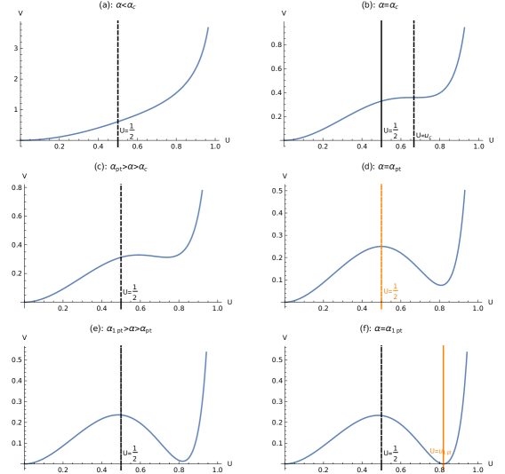
Figure 1: Effective potential for different values of temperature and associated phase transitions. The graphs are drawn for $q=4$.

At every positive value of $\alpha$, $V(u)=0$ when $u=0$ and $V(u)$ diverges as $u$ approaches unity from below. However the qualitative behaviour of the function $V(u)$ for values between zero and unity depends sensitively on $\alpha$.

It is easily verified that for $\alpha\leq\alpha_{c}=\frac{(q-1)^{q-1}}{4(q-2)^{q-2}}$ the function $V(u)$ increases monotonically as $u$ increases from $0$ to unity (see Fig 1 (a)). It follows that when $\alpha\leq\alpha_{c}$ the only saddle point lies at $u=0$. In this case the saddle point value of the partition function is $Z(x)=1$ (see below for a discussion of fluctuations about this saddle point value).

At $\alpha=\alpha_{c}$ the potential $V(u)$ develops a point of inflection at $u=u_{c}=\frac{q-2}{q-1}$ (see Fig. 1 (b)). Note that $u_{c}>\frac{1}{2}$. At this value of $\alpha$ we have a new saddle point in the gapped phase.

As $\alpha$ is increased above $\alpha_{c}$ the point of inflection at $u=u_{c}$ splits up into two saddle points; a local maximum at $u=u_{max}<u_{c}$ and a local minimum at $u=u_{min}>u_{c}$ (see Fig. 1 (c)). To start with both saddle points are in the gapped phase. We refer to the saddle point at $u_{max}$ as the upper saddle and the saddle point at $u_{min}$ as the lower saddle.

As $\alpha$ is increased further the value of $u_{min}$ continues to increase while the value of $u_{max}$ continues to decrease. At $\alpha=\alpha_{pt}=2^{q-3}>\alpha_{c}$, $u_{max}=\frac{1}{2}$. For $\alpha>\alpha_{pt}$, $u_{max}<\frac{1}{2}$ and the upper saddle makes a Gross Witten Wadia phase transition into the wavy phase (see Fig 1 (d)).

Finally, when the new saddle point at $u=u_{c}$ is first nucleated, we have $V(u_{c})>0$. As $\alpha$ is increased $V(u_{min})$ decreases below this value. At $\alpha=\alpha_{1pt}=$ we have $V(u_{min})=0$ (see Fig 1(f)). For larger values of $\alpha$, $V(u_{min})<0$ and our matrix model undergoes a first order phase transition from the saddle at $u=0$ to the saddle at $u=u_{min}$. Note that at $\alpha=\alpha_{1pt}$ (i.e. at the ‘Hawking Page transition temperature’) the saddle at $u=u_{max}$ is already in the the wavy phase when $q=4$ but is still in the gapped phase for $q>4$.

3.3 Thermodynamics in the canonical ensemble

The thermodynamics of our system in the canonical ensemble follows immediately from the nature of the function $V(u)$ as a function of $\alpha$ described at the end of the last section. For convenience we discuss the phase diagram of our system as a function of $\alpha$ rather than temperature (recall that $\alpha$ is defined by the relations $e^{-\beta m}=x=\frac{\alpha}{pN^{q-3}}$).

For $\alpha<\alpha_{c}$ the saddle at $u=0$ is the only saddle point in the theory (see Fig 1 (a)). For $\alpha_{c}<\alpha<\alpha_{pt}$ there are two additional saddle points at $u=u_{min}$ and $u=u_{max}$ with $\frac{1}{2}<u_{max}<u_{min}<1$. The saddle point at $u=u_{max}$ is a local maximum and $V(u_{max})>0$ (see Fig 1 (c)). The saddle point at $u=u_{min}$ is a local minimum and however $V(u_{min})>0$. Both these saddles are subdominant compared to the flat saddle in this range of $\alpha$.

For $\alpha_{pt}<\alpha<\alpha_{1pt}$ the two new phases continue to be subdominant compared to the phase at $u=0$; in this range, however, the solution at $u=u_{max}<\frac{1}{2}$ is now in the wavy phase (see Fig 1 (e)).

At $\alpha=\alpha_{1pt}$ we have $V(u_{min})=0$. For $\alpha>\alpha_{1pt}$ $V(u_{min})<0$, so the solution at $u=u_{min}$ is the dominant saddle point. Our system undergoes a phase transition at $\alpha=\alpha_{1pt}$ (see Fig 1 (e)). The value of $\alpha_{1pt}$ is given as a function of $q$ by

$$\alpha_{1pt}=\frac{1}{4}(q-1)w\left[1-\frac{1}{(q-1)w}\right]^{-(q-2)},\ \ w=-W_{-1}\left[-\frac{2\exp\left[{-\frac{(q+1)}{2(q-1)}}\right]}{q-1}\right],$$ (77)

where $W_{n}$ is the productlog function.

3.4 Thermodynamics in the microcanonical ensemble

In this subsection we compute the density of states as a function of energy corresponding to each of the saddle points described in the previous subsection. In order to do this we use the thermodynamical relations

$$E(\alpha)=\alpha\partial_{\alpha}\ln Z(\alpha)\,~{}~{}~{}S(\alpha)=\left(\ln Z(\alpha)-E(\alpha)\ln\frac{\alpha}{N^{q-3}p}\right),$$ (78)

where $E$ is the eigenvalue of $\frac{H}{m}$. We invert the first of these equations to solve for $\alpha(E)$, and then plug this solution into the second equation to obtain $S=S(E)$. For the trivial saddle, the saddle value of $S(E)$ is trivial, so we include the contribution of fluctuations around this saddle.

3.4.1 The saddle at $u=0$

The saddle point at $u=0$ exists at every value of $\alpha$. In this case the saddle point values of the energy and entropy both vanish so the first nontrivial contribution to the thermodynamics comes from the study of fluctuations about the saddle point. In this subsection - which is a bit of a deviation from the main flow of the (otherwise purely saddle point) computations of this paper we describe the relevant computations. For the purposes of this subsection - and this subsection only - we retreat away from the scaling limit (10) and work with the full matrix model (8) - or more precisely with its generalisation (9) which allows for bosonic as well as fermionic harmonic oscillators. Working with this generalised model we compute the fluctuations around the trivial saddle point $\operatorname{Tr}U_{m}^{n}=0$, i.e. $\rho^{n}_{m}=0$.

For the purposes of studying small fluctuations around this saddle point we work with the integral (62). The integral (62) can be simplified by making the variable change

$$\rho_{m}^{n}=\frac{\beta_{m}^{n}}{N}$$ (79)

The point of the scaling (79) is that it eliminates all explicit factors of $N$ from the integral (62). It follows that - at least for the purposes of the perturbative Wick contraction evaluations we perform in this subsection - at any finite order in perturbation theory the integral over $\beta^{m}_{n}$ receives significant contributions only from values of $\beta^{m}_{n}$ of order unity. Note however that if $\beta^{m}_{n}$ are of order unity then $\rho^{m}_{n}$ are of order $\frac{1}{N}$ and so are very small. We can thus safely integrate over all values of $\beta^{m}_{n}$ without worrying about boundaries to the domain of integration. In other words (62) may be rewritten in terms of these scaled variables

$$\begin{split}&Z(x)=\prod_{n=1}^{\infty}F_{n}(x),\\ &F_{n}(x)=\begin{cases}M_{n}\displaystyle\int\prod_{m=1}^{q-1}d\beta_{m}^{n}\exp\left(-\sum_{m=1}^{q-1}\frac{|\beta_{m}^{n}|^{2}}{2n}+N_{F}x^{n}\frac{\left(\prod_{m=1}^{q-1}\beta^{n}_{m}\right)+\text{c.c}}{n}\right)&~{}~{}~{}n~{}~{}{\rm odd}\\ M_{n}\displaystyle\int\prod_{m=1}^{q-1}d\beta_{m}^{n}\exp\left(-\sum_{m=1}^{q-1}\frac{|\beta_{m}^{n}|^{2}}{2n}-N_{F}x^{n}\frac{\left(\prod_{m=1}^{q-1}\beta^{n}_{m}\right)+\text{c.c}}{n}\right)&~{}~{}~{}n~{}~{}{\rm even}.\\ \end{cases}\end{split}$$ (80)

The expressions for $F_{n}$ above involve an integral with the usual measure $dzd{\bar{z}}$ for the complex variable $\beta^{n}_{m}$. The integral is taken over the whole complex plane. The $x$ independent normalisation constant $M_{n}$ above are chosen to ensure that normalisation of Haar measure,i.e, $F_{n}(0)=1$ .

The expressions for $F_{n}$ presented in (80) are formal as the integrals that define $F_{n}$ do not converge. However this fact does not bother us, as we are not really interested in the the expression for $Z(x)$ but only in the coefficients in of $x^{k}$ for each $k$ in that expression. Each of these coefficients is easily obtained (by Taylor expanding the non Gaussian terms in the integrands in the formulas for $F_{n}$ above and performing all integrals using Wicks theorem. We find

$$F_{n}(x)=\sum_{k=0}^{\infty}x^{2kn}\left(p^{2}(2n)^{q-3}\right)^{k}(k!)^{q-3},~{}~{}~{}p\equiv N_{F},$$ (81)

Let $E$ denote the eigenvalues of $\frac{H}{m}$; in other words $E$ is the energy of our theory in units of the oscillator mass (or frequency). It follows from (81) that the functions $F_{n}(x)$ represent the partition function of a system whose entropy as a function of energy is given by $S_{n}(E)$ where

$$e^{S_{n}(E)}=\left(\frac{E}{2n}!\right)^{q-3}\left(p^{2}(2n)^{q-3}\right)^{\frac{E}{2n}}.$$ (82)

At large $E$ ( i.e. when $E\gg 2n$) we may use Sterling’s approximation to simplify (82) to obtain the asymptotic formula

$$S_{n}(E)=(q-3)\frac{E}{2n}\ln\left(\frac{E}{2n}\right)+\frac{E}{2n}\left(-(q-3)+2\ln p+(q-3)\ln(2n)\right).$$ (83)

Notice that the density of states grows faster than exponentially as a function of energy, explaining the divergence of the integrals that define $F_{n}$ (or, equivalently, explaining why the sums in (81) are divergent at every $x$ no matter how small.

As the partition function of our system is simply the product over the functions $F_{n}$, the entropy of our system at large energies is obtained by distributing the available energy $E$ among the various systems $S_{n}$ in such a way as to maximise the entropy. A glance at (83) is sufficient to convince oneself that the best one can do is to put all available energy into the ‘system’ $S_{1}$. It follows that for $E\gg 1$, the contribution of the saddle point at $u_{1}=0$ to the entropy of the system is

$$S(E)=S_{1}(E)=(q-3)\frac{E}{2}\ln\left(\frac{E}{2}\right)+\frac{E}{2}\left((\ln(2)-1)(q-3)+2\ln p\right).$$ (84)

The saddle at $u=0$ is exceptional in that it is trivial as a saddle point; in order to determine the thermodynamics of this ‘phase’ we had to perform the one loop expansion about this saddle point. The remaining saddle points we will study in this section are nontrivial even at leading order, and so will be analysed only within the strict saddle point approximation. In the rest of this subsection we also return to the study of the strict scaling limit (10).

3.4.2 The wavy phase

In this subsection we study the thermodynamics of the wavy saddle, i.e. the saddle point at $u=u_{max}$ for $\alpha>\alpha_{pt}=2^{q-3}$. The contribution of this saddle point to partition function is

$$\ln Z(\alpha)=-\frac{N^{2}}{2}(q-3)\alpha^{-\frac{2}{q-3}}.$$ (85)

The energy of the corresponding phase is given by

$$E(\alpha)=\alpha\partial_{\alpha}\ln Z(\alpha)=\frac{N^{2}}{\alpha^{\frac{2}{q-3}}},$$ (86)

Note that the energy is a decreasing function of $\alpha$ so that this phase has a negative specific heat. As this phase exists only for $\alpha>\alpha_{pt}$ it follows that the energy in this phase is bounded from above by

$$E_{pt}\equiv E(\alpha_{pt})=\frac{N^{2}}{4}.$$ (87)

The entropy of this phase is given by

$$S(\alpha)=\left(\ln Z(\alpha)-E(\alpha)\ln\frac{\alpha}{N^{q-3}p}\right).$$ (88)

Eliminating $\alpha$ between (86) and (88) we obtain

$$S(E)=(q-3)\left[\frac{E}{2}\ln\left(\frac{E}{2}\right)-\frac{E}{2}\right]+E\ \log p+(q-3)\frac{E}{2}\ln(2).$$ (89)

Note that (89) is in perfect agreement with (84). This match strongly suggests that the formula (89) is correct for all values of $E$ in the range

$$\ 1\ll E<\frac{N^{2}}{4}.$$ (90)

3.4.3 The gapped phase

The analysis of this section applies to the saddle point at $u=u_{max}$ for $\alpha\leq\alpha_{pt}$ and to the saddle point at $u_{min}$. The partition function of this saddle is given by plugging the solution of the equation

$$u=1-\dfrac{1}{4\alpha u^{q-2}}\ ,\quad u\geq\frac{1}{2}$$ (91)

into the formula

$$\ln Z=-\frac{N^{2}}{2}\left[(q-1)\left(\dfrac{1}{4}-\dfrac{1}{2}\ln\left[2(1-u)\right]\right)-2\alpha u^{q-1}\right].$$ (92)

As we have explained above, for $\alpha<\alpha_{c}=\frac{(q-1)^{q-1}}{4(q-2)^{q-2}}$ there are no legal solutions to (91). For $\alpha_{c}<\alpha<\alpha_{pt}=2^{q-3}$ there are two legal solutions and for $\alpha>\alpha_{pt}$ there is a single legal solution to this equation. After the partition function is obtained one obtains the energy and entropy of the solution using the thermodynamical formulae

$$E(\alpha)=\alpha\partial_{\alpha}\ln Z(\alpha)\ ,~{}~{}~{}S(\alpha)=\left(\ln Z(\alpha)-E(\alpha)\ln\frac{\alpha}{N^{q-3}p}\right).$$ (93)

Eliminating $\alpha$ from the expressions obtained in (93) we find the entropy $S$ as a function of the energy. This function $S=S(E)$ is difficult to find explicitly simply because (91) is difficult to solve. The procedure described above, however, implicitly defines this function. It is not difficult to convince oneself that there is a single saddle point of this nature for every energy $E>\frac{N^{2}}{4}$ and that the function $S(E)$ is an analytic function of energy for every energy greater than $\frac{N^{2}}{4}$.

While explicit formulae are difficult to obtain in general, they are easy to obtain in three special limits which we now describe

A. The solutions with $\alpha$ near $\alpha_{pt}$ i.e. ($E$ near $E_{pt}$):

At $\alpha=\alpha_{pt}$ (91) admits the solution $u=\frac{1}{2}$. (This is a solution at $u=u_{max}$, i.e. the solutions that is a local maximum). It follows that at $\alpha=\alpha_{pt}-\delta\alpha$, (91) admits a solution with $u=\frac{1}{2}+\delta u$. Here $\delta u$ is solved order by order in $\delta\alpha$. A few lines of standard algebra gives:

$$\begin{split}S\left(E_{pt}+\delta E\right)=&-\frac{1}{4}N^{2}\left[\log\left(\frac{2^{q-3}N^{3-q}}{p}\right)+\frac{q-3}{2}\right]-\log\left[\frac{2^{(q-3)/2}N^{3-q}}{p}\right]\delta E\\ &~{}~{}~{}~{}~{}~{}+\frac{2(q-3)}{2N^{2}}\left(\delta E\right)^{2}+\frac{4(7-3q)}{6N^{4}}\left(\delta E\right)^{3}+\ldots\end{split}$$ (94)

Comparing (94) and (89), it is easily verified that while $S(E)$, $S^{\prime}(E)$ and $S^{\prime\prime}(E)$ are continuous at $E=\frac{N^{2}}{4}$, $S^{\prime\prime\prime}(E)$ is discontinuous. In that sense the function $S(E)$ has a third order phase transition’ at $E=\frac{N^{2}}{4}$. Further taking the limit:

$$\lim_{\epsilon\to 0^{+}}S^{{}^{\prime\prime\prime}}\left(\frac{N^{2}}{4}-\epsilon\right)=\frac{4(6-2q)}{N^{4}},\quad\lim_{\epsilon\to 0^{+}}S^{{}^{\prime\prime\prime}}\left(\frac{N^{2}}{4}+\epsilon\right)=\frac{4(7-3q)}{N^{4}}$$ (95)

This discontinuity is a consequence of the fact that the saddle point undergoes a Gross Witten Wadia transition at this energy.

B. The solutions with $\alpha$ near $\alpha_{c}$ (i.e. $E$ near $E_{c}$):

At $\alpha=\alpha_{c}$ (91) admits the solution $u=\frac{q-2}{q-1}$. For $\alpha=\alpha_{c}+\delta\alpha$ the (91) admits two solutions near this critical solution at $u=u_{c}+\delta u$; these are the solutions at $u=u_{max}$ and $u=u_{min}$ respectively. A careful calculation shows $E,S$ as a function of $\alpha$ are different for this two branches but $S$ as a function of $E$ is same for both of them and given by:

$$\begin{split}S\left(E_{c}+\delta E\right)=&\frac{1}{4}N^{2}\left[-(q-2)\log\left(\frac{(q-2)^{2-q}(q-1)^{q-1}N^{3-q}}{4p}\right)+(q-1)\log\left(\frac{2}{q-1}\right)+\frac{(q-3)}{2}\right]\\ &-\log\left[\frac{(q-2)^{2-q}(q-1)^{q-1}N^{3-q}}{2^{(q+1)/2}p}\right]\left(\delta E\right)+\left[-\frac{8}{3N^{4}(q-2)(q-1)}\right]\left(\delta E\right)^{3}+\ldots\end{split}$$ (96)

Note that (96) is completely smooth around $E=E_{c}=\frac{1}{4}N^{2}(q-2)$.

C. The solutions with $\alpha\gg 1$ (i.e. $E\gg\frac{N^{2}}{2}$):

At $\alpha\gg 1$ (91) admits the solution near $u=1$; this is the thermodynamically dominant saddle at $u=u_{max}$. Setting $u=1-\delta u$, $\delta u$ is solved to give as series in $\frac{1}{\alpha}$:

$$\delta u=\left(\frac{1}{4}\right)\alpha^{-1}+\left(\frac{q-2}{16}\right)\alpha^{-2}+\ldots$$ (97)

It follows that:

$$\begin{split}\ln Z(\alpha)&=N^{2}\alpha+\left(-\frac{1}{4}N^{2}(q-1)\right)\log(\alpha)+\ldots,\\ E(\alpha)&=N^{2}\alpha+\left(-\frac{N^{2}(q-2)(q-1)}{32}\right)\alpha+\ldots,\\ S(\alpha)&=\left(-N^{2}\right)\alpha\log(\alpha)+\left(N^{2}\left(1+\log\left(2pN^{q-3}\right)\right)\right)\alpha+\ldots\end{split}$$ (98)

which gives

$$S(E) = E-E\log\left(\frac{E}{pN^{q-1}}\right)-\frac{N^{2}}{2}\bigg{[}\frac{q-1}{2}\log\left(\frac{2E}{N^{2}}\right)+\frac{3}{4}(q-1)+\frac{1}{8}(q-1)\left(\frac{2E}{N^{2}}\right)^{-1}\bigg{]}+\ldots~{}~{}~{}~{}~{}~{}~{}~{}~{}$$ (99)

3.4.4 Entropy as a function of energy for $E\gg\frac{N^{2}}{2}$

We have verified above that for $E\gg\frac{N^{2}}{2}$ the saddle point for the eigenvalue distribution function becomes very peaked and so is well approximated by a delta function. Whenever the eigenvalue distribution becomes so peaked effect of the holonomies on the partition function of the system can be ignored. It follows that for energies much greater than $N^{2}$ the partition function of our system is simply that of $N_{F}N^{q-1}$ complex fermionic oscillators. The partition function for our system thus reduces to

$$\ln Z(x)=N_{F}N^{q-1}\ln(1+x),$$ (100)

For $x\ll 1$ (100) reduces to

$$\ln Z(x)=~{}x~{}p~{}N^{q-1}.$$ (101)

Substituting $x=\frac{\alpha}{N^{q-3}p}$ we find that (101) agrees precisely with the leading term in the first line of (98):

$$\ln Z(\alpha)=N^{2}\alpha.$$ (102)

The energy of the corresponding phase is given by

$$E(\alpha)=\alpha\partial_{\alpha}\ln(Z(\alpha))=N^{2}\alpha.$$ (103)

The entropy of this phase is given by

$$S(\alpha)=\ln Z(\alpha)-E(\alpha)\ln\frac{\alpha}{N^{q-3}p}=N^{2}\left(1-\log\left(\frac{\alpha}{pN^{q-3}}\right)\right)\alpha.$$ (104)

Eliminating $\alpha$ between (103) and (104) we obtain

$$S(E)=E\left(1-\log\left(\frac{E}{pN^{q-1}}\right)\right).$$ (105)

Note that (105) matches with the leading and 1st subleading term in (99).

4 The holonomy effective action with weak interactions

In the previous section we studied the free energy of the mass deformed SYK model in the zero coupling $\frac{J}{m}=0$. In this section we will study corrections to the results of the previous section in a power series expansion in the coupling constant. For simplicity we also study the special case $N_{F}=1$ in (7) .

In principle the leading large $N$ contribution to $S_{\text{eff}}$ is given as follows (we restrict attention to the massless case for simplicity in this paragraph). Consider the gap equation (20). We are instructed to solve this gap equation on a thermal circle, subject to the requirement that the solution respect the boundary conditions

$$\begin{split}&G\left(t_{1}+\frac{\beta}{2},t_{2}\right)=-UG\left(t_{1}-\frac{\beta}{2},t_{2}\right)\\ &G\left(t_{1},t_{2}+\frac{\beta}{2}\right)=-G\left(t_{1},t_{2}-\frac{\beta}{2}\right)U^{-1}\\ &\Sigma\left(t_{1},t_{2}+\frac{\beta}{2}\right)=-U\Sigma\left(t_{1},t_{2}-\frac{\beta}{2}\right)\\ &\Sigma\left(t_{1}+\frac{\beta}{2},t_{2}\right)=-\Sigma\left(t_{1}-\frac{\beta}{2},t_{2}\right)U^{-1}\\ \end{split}$$ (106)

We must then plug this solution into (18) and the corresponding result is represented by $S_{\text{eff}}(U).$ While this prescription is clear it is rather difficult to implement in practice. In order to get some intuition for the effect of interactions on $S_{\text{eff}}(U)$ present some perturbative results for this object.

The thermal partition function of theory (7) is given, as usual, by the Euclidean path integral of the theory on a thermal circle of circumference $\beta$. The free result (8) is obtained by integrating out all fermions at at ‘one loop’ (i.e. by computing fermionic determinants -we explain how this works in more detail below). Corrections to (8) are obtained by including the contribution of more general diagrams.

It was demonstrated in Witten:2016iux that, in the strict large $N$ limit of interest to this paper, the only graphs that contribute are melonic graphs. One way of organising the graphs that contribute to our computation is by the number of melons a graph contains. We will refer to a graph with $n$ melons as an $n^{th}$ order graph. Such graphs are proportional to $J^{2n}$. As in the previous section we will be interested in the effective action as a function of holonomies, $S_{\text{eff}}(U)$. Let the contribution to $S_{\text{eff}}(U)$ from graphs of $n^{th}$ order be denoted by $S_{n}(U)$. We have

$$S_{\text{eff}}(U)=\sum_{n=0}^{\infty}S_{n}(U).$$ (107)

As in the previous section we will principally be interested in the partition function in the scaling limit (10). In this limit the temperature is very small and so $\beta$ is very large $\beta\sim\ln N$. For this reason it is important to keep track of explicit multiplicative factors of $\beta$ (as opposed, for instance, to factors of $x=e^{-\beta m}$) in our results. Below we will demonstrate that $n^{th}$ order graphs have at least one and at most $n$ explicit multiplicative factors of $\beta$. It follows that the contributions of $n^{th}$ order graphs to the effective action can be organised in series

$$S_{n}(U)=\frac{J^{2n}\beta^{n}}{m^{n}}\sum_{a=0}^{n-1}\left(\frac{1}{m\beta}\right)^{a}f^{n}_{a}(x,U)\equiv-\left(\frac{J}{m}\right)^{2n}F_{2n}(m\beta,x,U).$$ (108)

Substituting (108) into (107), we can rearrange the sum over graphs as

$$\begin{split}S_{\text{eff}}(U)&=\sum_{k=0}^{\infty}\left(\frac{J}{m}\right)^{2k}H_{k}(\frac{J^{2}\beta}{m},x,U),\\ H_{k}(\frac{J^{2}\beta}{m},x,U)&=\sum_{n=k}^{\infty}\left(\frac{J^{2}\beta}{m}\right)^{n-k}f_{k}^{n}(x,U).\end{split}$$ (109)

As we are interested in the scaling limit (10) it follows that:

$$\begin{split}&H_{k}\left(\frac{J^{2}\beta}{m},x,U\right)={\tilde{H}}_{k}\left(\frac{J^{2}\beta}{m}\right)x\prod_{i=1}^{q-1}\operatorname{Tr}U_{i},\\ &f_{k}^{n}(x,U)=f_{k}^{n}x\prod_{i=1}^{q-1}\operatorname{Tr}U_{i},\\ &H_{k}\left(\frac{J^{2}\beta}{m}\right)=\sum_{n=k}^{\infty}\left(\frac{J^{2}\beta}{m}\right)^{n-k}{\tilde{f}}_{k}^{n},\\ &S_{\rm eff}(U)=x\prod_{i=1}^{q-1}\operatorname{Tr}U_{i}\times\sum_{k=0}^{\infty}\left(\frac{J}{m}\right)^{2k}{\tilde{H}}_{k}\left(\frac{J^{2}\beta}{m}\right),\end{split}$$ (110)

where we will present an argument for the $u$ dependences asserted here below.

(110) represents an interesting reorganisation of usual perturbation theory. This reorganisation is particularly useful at small $\frac{J^{2}}{m^{2}}\ll 1$ but finite values of $\frac{J^{2}\beta}{m}$. As $\beta\sim\frac{m}{\ln N}$ in the scaling limit, it follows that $\frac{J^{2}\beta}{m}$ is fixed only for $\frac{J^{2}}{m^{2}}\sim\frac{1}{\ln N}$. At these small values of the coupling, $S_{\rm eff}(U)$ is well approximated by the first term in the expansion in (110), i.e. by the term proportional to ${\tilde{H}}_{0}$. We will explicitly evaluate ${\tilde{H}}_{0}$ in this section and so reliably determine the partition function when $\frac{J^{2}}{m^{2}}$ is in the parametric range described above.

In the rest of this section we present the results of our explicit perturbative computations. Although we are principally interested in the function $H_{0}$ in the scaling limit, to set notations and for practice we first present the results of simpler computations. To start with we work out the partition function at level zero and recover the free partition function of the previous section. We then work out the partition function at level 1 (i.e. including graphs with a single melon). Next we present our results at level 2 (i.e. including all graphs with two melons). Finally we turn to the problem of principal interest to us, namely the sum of the infinite set of graphs that generates $H_{0}$. As preparation for all these computations we first briefly discuss the structure of the free Greens function.

4.1 Free Greens Function

Consider the free fermionic Greens function

$$\langle\psi^{a}(t)\bar{\psi}_{b}(0)\rangle.$$

We work in a colour basis in which the holonomy $U$ is diagonal. In this basis in which the action of holonomies on the fermions is given by

$$\begin{split}U\psi^{a}&=e^{i\theta_{a}}\psi^{a},\\ U{\bar{\psi}}_{a}&=e^{-i\theta_{a}}\psi_{a}.\\ \end{split}$$ (112)

The free fermionic Greens function at finite temperature is given by

$$\langle\psi^{a}(t)\bar{\psi}_{b}(0)\rangle= G_{0}(t)\delta^{a}_{b},\ G_{0}(t)=f(t,m,\theta_{a}),\ \ \textit{for \ $-\beta\leq t\leq\beta$ }$$ (113)

where

$$f(t,m,\theta_{a})= \frac{1}{2}e^{-(m+i\theta_{a})t}\left[\text{sgn}(t)+\tanh\left(\frac{1}{2}(m+i\theta_{a})\beta\right)\right]$$ (114)

$$= \frac{e^{-(m+i\theta_{a})t}}{1+x\ e^{-i\theta_{a}\beta}}\left[\Theta(t)-\Theta(-t)\ x\ e^{-i\theta_{a}\beta}\right].$$

Note that the function $f$ obeys the identity

$$f\left(\frac{\beta}{2}+t,m,\theta_{a}\right)=-f\left(-\frac{\beta}{2}+t,m,\theta_{a}\right)\ \ \textit{for \ $0\leq t<\frac{\beta}{2}$},$$ (115)

from which it follows that the Greens function is antiperiodic on the circle as required on physical grounds.

Note that we have presented the Greens function only in the ‘fundamental domain’ $-\beta<t<\beta$. Our fermionic Greens function is taken by definition to be a periodic function of $t$ with period $2\beta$; this property plus the explicit results (113) and (114) can be used to define the Greens function at every value of Euclidean time as required. The extended Greens function defined in this manner has singularities at $t=n\beta$ for every integral value of $n$, and is smooth everywhere else.

Note also that the ‘reversed’ Greens function $\langle{\bar{\psi}}_{a}(t)\psi^{b}b(0)\rangle$ is also given in terms of the function $G_{0}$ by the formula

$$\langle{\bar{\psi}}_{a}(t)\psi^{b}(0)\rangle=-G_{0}(-t)\delta^{b}_{a}.$$ (116)

This formula is also manifestation of symmetry of mass deformed SYK Lagrangian under the simultaneous swaps ${\bar{\psi}}\leftrightarrow\psi$, $U\leftrightarrow U^{-1}$, $m\leftrightarrow-m$.

4.2 Level zero: Free theory

In this brief subsection we compute $S_{\text{eff}}$ at one loop, i.e. in the free theory. The result for $S_{\text{eff}}(U)$ was already presented in the previous subsection; we obtain that result here from a one loop computation as a simple practice exercise. Let

$$\omega_{n}=\frac{2\pi}{\beta}\left(n+\frac{1}{2}\right).$$ (117)

The fields $\psi^{a}$ and ${\bar{\psi}}_{a}$ can be independently expanded in Fourier space as

$$\psi(t)=\sum_{n}\psi^{n}e^{-i\omega_{n}t}\ ,\ \bar{\psi}(t)=\sum_{n}\bar{\psi}_{n}e^{+i\omega_{n}t}.$$ (118)

When substituted the free part of action (7) becomes

$$S=\sum_{n,a}\bar{\psi}_{a,n}[\beta(-i\omega_{n}+m+i\theta_{a})]\psi^{a,n}.$$ (119)

Fermionic integration gives:

$$Z_{F}= \prod_{a}\prod_{n=-\infty}^{n=+\infty}\left[\beta(-i\omega_{n}+m+i\theta_{a})\right]$$ (120)

$$= \prod_{a}\prod_{n=-\infty}^{n=+\infty}\left[-i(2\pi n+\pi)+m\beta+i\theta_{a}\beta\right]$$

$$= \prod_{a}\prod_{n=-\infty}^{n=+\infty}\left[-i2\pi n+c(\theta_{a})\right]$$

$$= \prod_{a}c(\theta_{a})^{2}\prod_{n=1}^{n=+\infty}\left[(-i2\pi n+c(\theta_{a}))(+i2\pi n+c(\theta_{a}))\right]$$

$$= \prod_{a}c(\theta_{a})^{2}\prod_{n=1}^{n=+\infty}\left[(2\pi n)^{2}+c(\theta_{a})^{2}\right]$$

$$= \prod_{a}c(\theta_{a})^{2}\left(\prod_{n=1}^{n=+\infty}(2\pi n)^{2}\right)\prod_{n=1}^{n=+\infty}\left[1+\left(\frac{c(\theta_{a})/2}{\pi n}\right)^{2}\right]$$

$$= \prod_{a}c(\theta_{a})^{2}\left(\prod_{n=1}^{n=+\infty}(2\pi n)^{2}\right)\left[\frac{\sinh\frac{c(\theta_{a})}{2}}{\frac{c(\theta_{a})}{2}}\right]$$

$$= N\prod_{a}\left[\sinh\frac{c(\theta_{a})}{2}\right]\sim\prod_{a}e^{\frac{c(\theta_{a})}{2}}(1-e^{-c(\theta_{a})}),$$

where

$$c(\theta_{a})=m\beta+i\theta_{a}\beta-i\pi$$

and

$$N=\prod_{a}\prod_{n=1}^{n=+\infty}(2\sqrt{2}\pi n)^{2}$$

is an infinite holonomy independent constant. As for every $\theta_{a}$ there is $-\theta_{a}$ to be taken into account $\prod_{a}e^{\frac{c(\theta_{a})}{2}}$ becomes independent of holonomy. Keeping only holonomy dependent terms

$$\ln Z=\sum_{a}\log[1+xe^{-i\theta_{a}\beta}]\ ,\ \ x=e^{-m\beta},$$ (121)

In other words

$$\ln Z=\operatorname{Tr}\ln[1+xU].$$ (122)

Expanding (122) in a power series in $x$ we recover (8) at $N_{F}=1$. In the scaling limit we recover (64).

4.3 Level one: single melon graphs

The contributions of graphs with a single melon to the Free energy is given by

$$F_{2}=\frac{1}{2!}\ ^{2}C_{\frac{2}{2}}\ (-1)^{q/2}q\ m^{2}\int\prod_{k=1}^{q}G_{0}(t_{1}-t_{2},\theta_{a_{k}})\ dt_{1}dt_{2},$$ (123)

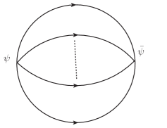
Figure 2: Single loop contribution to free energy.

In this graph we contract each of fields in the interaction vertex $\psi^{q}$ with one of the fields in ${\bar{\psi}}^{q}$. Consider any particular $\psi$ field. This $\psi$ field has to contract with one of the $q$ ${\bar{\psi}}$ fields in the second interaction vertex. It is thus clear that there are $q$ choices for this contraction (the choices of which ${\bar{\psi}}$ our specified $\psi$ pairs up with). Once this choice has been made, if we are interested - as we are- in graphs that contribute only at leading order in large $N$ there are no further choices in our contraction. Recall that every one of the remaining $\psi$’s (respectively $\bar{\psi}$’s) has exactly one colour common with the $\psi$ (resp $\bar{\psi}$) that we have just contracted together. The leading large $N$ behaviour is obtained only if the $\psi$ that shares any given gauge index with our special contracted $\psi$ is now contracted with the $\bar{\psi}$ that shares the same gauge index with the special contracted ${\bar{\psi}}$. This rule specifies a unique contraction structure for the remaining fields. It follows that, up to a sign, the symmetry factor is simply $q$. The sign in question is simply $(-1)^{(q-1)+(q-2)+..+1}$ Recalling that $q$ is even, it is easy to see that this phase $=(-1)^{q/2}$.

The integral in (123) is very easy to perform. To see this note that the analytic structure of the integrand as a function of $t=t_{1}-t_{2}$ takes the form

$$e^{-qmt}(A_{q}\ \text{sgn}(t)+B_{q}),$$

for various different values of $q$. The integrand is integrated from $-\frac{\beta}{2}$ to $\frac{\beta}{2}$. The integral over $t_{1}+t_{2}$ produces an overall factor of $\beta$. The integrals are all trivial to do; evaluating them we find the final answer

$$F_{2}=\frac{(-1)^{q/2}}{2!}\ ^{2}C_{\frac{2}{2}}\ q\,m\beta\ I^{(2)}_{1}(q,x),$$ (124)

where

$$I^{(2)}_{1}(q,x)=\frac{1-x^{q}}{q}{\rm Tr}_{F}\prod_{k=1}^{q}\left(\frac{1}{1+x\tilde{U}_{k}}\right).$$ (125)

The expression $\operatorname{Tr}_{F}(...)$ in the equation above represents the trace over an operator built on a particular Auxiliary Hilbert space. The operator in question is a function of the elementary operators ${\tilde{U}}_{k}$ that act on this Hilbert space. We will now carefully define the relevant Hilbert space and the operators ${\tilde{U}}_{k}$ and so give meaning to (125).

The operators ${\tilde{U}}_{k}$ in (125) have the following meaning. These operators are unitary operators that act on a vector space whose dimensionality is $N^{\frac{q}{2}(q-1)}$. The vector space in question is the tenor product of $q-1$ factors, each of which has dimension $N^{\frac{q}{2}}$. Each factor described above is associated with one of the $q-1$ gauge groups. Let us focus on any one gauge group, say the first. The factor associated with this gauge group consists of $\frac{q}{2}$ distinct factors of isomorphic $N$ dimensional spaces on which the $N\times N$ holonomy matrices of the first gauge group naturally act.

Recall that each $\psi$ field that appears in an interaction has exactly one gauge index contraction with every other $\psi$ field. This means, in particular, that the indices of gauge group 1 are contracted between $\frac{q}{2}$ pairs of $\psi$s. This fact is the origin of the $\frac{q}{2}$ distinct factors of the space on which the holonomy matrices of the first gauge group act.

With all this preparation we now explain the form of the operators $\tilde{U}_{k}$. Each $\tilde{U}_{k}$ acts as $U_{1}$ (the holonomy of the first $O(N)$ gauge group) on one of the $\frac{q}{2}$ copies of the $N$ dimensional vector space associated with the first $O(N)$, and as identity on the remaining $\frac{q}{2}-1$ copies of this space. In a similar fashion it acts as $U_{2}$ on one of the $\frac{q}{2}$ copies of the $N$ dimensional vector space associated with the second $O(N)$, and as identity on the remaining $\frac{q}{2}-1$ copies of this space. And so on. Exactly two $\tilde{U}_{k}$s act as $U_{1}$ on the same Hilbert space. Exactly two $\tilde{U}_{k}$s act as $U_{2}$ on the same Hilbert space, etc. Finally every two $\tilde{U}_{k}$s act on the same Hilbert space for one and only one gauge group. The symbol ${\rm Tr}_{F}$ in that equation denotes the trace over the full $N^{\frac{q}{2}(q-1)}$ dimensional Hilbert space.

From a practical point of view it is less complicated to use the definitions of the ${\tilde{U}}_{k}$ operators than it might at first seem. We could, for instance, expand the result (125) in a power series in $x$. The formal looking expressions of traces of sums of products of ${\tilde{U}}_{k}$ operators that appear as coefficients in this expansion can easily be evaluated in terms of traces of powers of the holonomy matrices $U_{1}\ldots U_{q-1}$ of the factors of $O(N)$.

A little thought will allow the reader to convince herself that the rules described above imply that, for instance

$${\rm Tr}\left(\sum_{k=1}^{q}{\tilde{U}}_{k}\right) = qN^{\frac{(q-2)(q-1)}{2}}{\rm Tr}U_{1}{\rm Tr}~{}U_{2}\ldots{\rm Tr}U_{q-1},$$ (126)

$${\rm Tr}\left(\sum_{k_{1}\neq k_{2}}^{q}{\tilde{U}}_{k_{1}}{\tilde{U}}_{k_{2}}\right) = qN^{\frac{q^{2}-5q+6}{2}}\left[\prod_{k=1}^{q-1}{\rm Tr}U_{1}^{2}~{}({\rm Tr}U_{2})^{2}\ldots({\rm Tr}U_{q-1})^{2}\right.$$ (127)

$$\left.~{}~{}~{}~{}~{}~{}~{}~{}~{}~{}~{}+(1\leftrightarrow 2)+(1\leftrightarrow 3)+\ldots(1\leftrightarrow q-1)\right],$$

$${\rm Tr}\left(\sum_{k=1}^{q}{\tilde{U}}^{2}_{k}\right) = qN^{\frac{(q-2)(q-1)}{2}}\left({\rm Tr}U^{2}_{1}~{}{\rm Tr}U^{2}_{2}\ldots{\rm Tr}U_{q-1}^{2}\right).$$ (128)

As an illustration of these rules let us evaluate the partition function in the low energy scaling limit described in the previous section. Recall that in the limit of interest $x\sim\frac{1}{N^{q-3}}$ and we are instructed to retain only those contributions to $S_{\text{eff}}(U)$ that are linear in $x$; terms of higher order in $x$ can be discarded. It follows that the partition function in this limit may be evaluated by Taylor expanding (125) in $x$ and discarding all terms that are quadratic or higher order in $x$. Using the first of (126) we conclude immediately that

$$F_{2}=\frac{(-1)^{q/2}}{2!}\ ^{2}C_{2/2}\ q\,m\beta\ N^{q-1}(-x)\prod_{m=1}^{q-1}\rho^{1}_{m}.$$ (129)

where $\rho^{1}_{m}=\frac{{\rm\operatorname{Tr}}U_{m}}{N}$ as in the previous section, and we have dropped the terms of order $x^{0}$ which are independent of $U_{m}$.

4.4 Level 2: 2 melon graphs

At level 2 we once again have contributions from a single Feynman diagram Fig 3. In order to evaluate this graph we must evaluate in integral

$$F_{4} = \frac{1}{4!}\ ^{4}C_{4/2}\ (-1)2(q^{2})^{2}\int\prod_{i=1}^{4}dt_{i}\ \left(\prod_{i=1}^{q-1}G_{0}(t_{12},\theta_{a_{i}})\right)\left(\prod_{i=1}^{q-1}G_{0}(t_{34},\theta_{b_{i}})\right)$$ (130)

$$~{}~{}~{}~{}~{}~{}~{}~{}~{}~{}~{}~{}~{}~{}~{}~{}~{}~{}~{}~{}~{}~{}~{}~{}~{}~{}~{}~{}~{}~{}~{}~{}~{}~{}~{}~{}~{}~{}~{}~{}~{}~{}~{}~{}~{}~{}~{}~{}~{}~{}~{}~{}~{}~{}~{}~{}~{}~{}~{}~{}~{}`\times G_{0}(t_{32},\theta_{c_{2}})G_{0}(t_{14},\theta_{c_{1}}).~{}~{}~{}~{}~{}~{}~{}~{}~{}$$

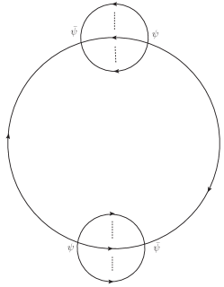
Figure 3: Two loop contribution to free energy.

We give some details of this expression and the evaluation of this integral in the Appendix B. We have completely evaluated this integral with the help of mathematica (see Appendix B.2 for arbitrary number of melons), but the final result for $S_{\text{eff}}(U)$ in the general case is too complicated to transfer to text. As before, however, the answer simplifies dramatically in the low energy scaling limit of the previous section (see Appendix B.1.1) and we find

$$F_{4}=\frac{(-1)}{4!}\ ^{4}C_{4/2}\ 2(q^{2})^{2}[m\beta\ I^{(4)}_{1}(q)+m^{2}\beta^{2}\ I^{(4)}_{2}(q)]\ N^{q-1}x\prod_{m=1}^{q-1}\rho^{1}_{m},$$ (131)

where

$$I^{(4)}_{1}(q)=-\frac{2}{q}(2q-3),$$ (132)

$$I^{(4)}_{2}(q)=-1.$$

Note that the final answer had two terms; one proportional to an overall factor of $\beta$ and the second proportional to $\beta^{2}$. In the next subsection we will argue that a graph at level $n$, in the low temperature scaling limit, has terms proportional to $\beta^{q}$ for $q=1\ldots n$.

4.5 The infinite sum $H_{0}$

We will now turns to a study of the free energy at level $n$. As in the previous subsection we will focus on the start at the low energy scaling limit of the previous section, and so retain only those terms in all graphs that are proportional to $x$. As we will see below, general graphs in the scaling limit and at level $n$ break up into different pieces that are proportional to $\beta^{k}$ for $k=1\ldots n$. We will further focus our attention on the graph with the largest power of $\beta$, i.e. in this subsection we will contribute that piece of the level $n$ answer that scales like $\beta^{n}x$. It turns out that this piece is rather easy to extract as we now explain.

Let us first recall that the propagator in our theory takes the following form:

$$\langle\psi_{a}(t){\bar{\psi}}^{b}(0)\rangle= \frac{e^{-(m+i\theta_{a})t}}{1+x\ e^{-i\theta_{a}\beta}}\left[\Theta(t)-\Theta(-t)\ x\ e^{-i\theta_{a}\beta}\right].$$ (133)

It will turn out (and we will see explicitly below) that the denominator in (133) only contributes at order $\beta^{n-1}$ or lower in free energy linear in $x$. For the purposes of the current subsection, therefore (where we wish to ignore terms at order $x^{2}$ or higher and only keep highest power of $\beta$) this denominator can be dropped, and we can work with the simplified propagator

$$\langle\psi_{a}(t){\bar{\psi}}^{b}(0)\rangle= e^{-(m+i\theta_{a})t}\left[\Theta(t)-\Theta(-t)\ x\ e^{-i\theta_{a}\beta}\right].$$ (134)

In this subsection we assume $m>0$; the case $m<0$ can be argued in a completely analogous manner with the role of $\psi$ and ${\bar{\psi}}$ reversed in the analysis below. In the computation of Feynman diagrams on the circle we will need to choose a ‘fundamental domain’ on the circle; our (arbitrary but convenient) choice of fundamental domain is

$$-\frac{\beta}{2}<t<\frac{\beta}{2}$$ (135)

Finally some terminology. We will call the part of the propagator (134) that is proportional to $\theta(t)$ the ‘forward’ (‘normal’) part of the propagator, and the part of the propagator proportional to $\theta(-t)$ the ‘reverse’ part of the propagator. Note that the normal part of the propagator ranges is modulus from $1$ to $\sqrt{x}$; it is maximum (i.e. unity) at $t=0$ and minimum (i.e. $\sqrt{x}$) at $t=\frac{\beta}{2}$. The modulus of the reverse part of the propagator varies in magnitude from $\sqrt{x}$ to $x$. It is minimum (i.e. equal to $x$) at $t=0$ and maximum (i.e. equal to $\sqrt{x}$) at $t=-\frac{\beta}{2}$.

With all this preparation we are now ready to isolate the parts of the level $n$ diagrams whose contribution is proportional to $x\beta^{n}$.

Figure 4: Circle diagram: a, b represents respectively insertions of $\psi$, $\bar{\psi}$. Direction of arrow is from $\psi$ to $\bar{\psi}$. The diagram is drawn for $q=4$.

To start with let us consider the simple $n^{th}$ level ring diagram depicted in Fig. 4. In this diagram we have $n$ $a$ type vertices and $n$ $b$ type vertices. In this graphs we have $q-1$ propagators connecting adjacent $a$ and $b$ type vertices, but only a single propagator connecting $b$ to $a$ type vertices.

Consider any propagator between $a$ and $b$ type vortices - which has $a$ type vertex $A$ at time $t_{1}$ and its adjacent $b$ type vertex $B$ at time $t_{2}$. Depending on whether $t_{1}>t_{2}$ or $t_{1}<t_{2}$, all the $q-1$ propagators from $A$ to $B$ are either simultaneously all reverse or simultaneously all normal. If all propagators are reverse, the modulus of these propagators is less than $\sqrt{x}^{q-1}<x$ (recall $q\geq 4$). It follows that configurations in which the propagators from $A$ to $B$ do not contribute in the scaling limit, and so all propagators from $A$ to $B$ must be normal. Given that these propagators are all normal their modulus is proportional to $e^{-m(q-1)|t_{1}-t_{2}|}$. It is intuitively clear that separating $t_{1}$ from $t_{2}$ over a finite fraction of the circle forces us to pay a high cost in factors of $x$; it can be shown (this will be clearer in a bit) that such configurations do not contribute to the result in the scaling limit. In the scaling limit we only receive contributions from configurations in which $|t_{1}-t_{2}|$ is of order $\frac{1}{m}$. It follows that for parametric purposes, we can simply regard $t_{1}$ and $t_{2}$ as the same point, replacing the integral over $t_{1}-t_{2}$ by $\frac{1}{m}$. For parametric purposes, in other words, each of the melons in Fig. 4 can be thought of as a single interaction vertex, inserted at a single ‘self energy vertex’, inserted at a single time, with effective an effective insertion factor of order $\frac{J^{2}}{m}$.

Now let us turn to the propagators between $b$ and $a$ type vertices. These are now $n$ different propagators connecting the effective self energy blobs described in the previous paragraph. Let the effective times of insertions of these self energy blobs be $T_{1}$, $T_{2}\ldots T_{n}$. Our graph is proportional to the product of $n$ propagators, the first from $T_{1}$ to $T_{2}$, the second from $T_{2}$ to $T_{3}$ $\ldots$ and the last from $T_{n}$ to $T_{1}+w\beta$ where $w$ is an integer. As each reverse propagator contributes a factor of at least $\sqrt{x}$ to the integrand, no more than two of these propagators can be reverse.

Let us first consider diagrams in which all propagators are forward. As all propagators move forward in time, the final propagator in the sequence must end not at time $T_{1}$ but at time $T_{1}+w\beta$ where $w$ is a positive integer. The modulus of the product of these propagators is then easily seen to be proportional to $e^{-wm\beta}=x^{w}$. In the scaling limit of interest to us, the only option is $w=1$. Once we set $w=1$, the integrand of the diagram is now independent of the effective insertion times $T_{i}$. The integral over these $n$ insertion times thus gives a factor $\beta^{n}$, and the contribution of the graph in question is proportional to $x\beta^{n}$ as desired.

Now let us consider diagrams in which one of the propagators between the effective self energy vertices is reverse, and the rest are forward. It is easy to verify that the modulus of the product of propagators in such a graphs is proportional to $xe^{-wm\beta}$ where $w=0,1,\ldots$. In the scaling limit under consideration we are interested only in $w=0$. Once again the modulus of these graphs is independent of the insertion positions of the effective self energy vertices, and integration over their locations produces a result proportional to $x\beta^{n}$ as required.

Diagrams in which two of the propagators are reverse are kinematically very constrained. Similar argument as above shows these graphs are proportional to $x$ only if $w=-1$,i.e, if the two reverse propagators each have length $\frac{\beta}{2}$ (up to corrections of order $\frac{1}{m}$) and so all the forward propagators have length zero, again up to corrections of order $\frac{1}{m}$. These constraints ensure that such graphs are proportional to $\beta$ but no higher power of $\beta$ (certainly not $\beta^{n}$) and so are not of interest to the current section.

In summary, graphs of the form depicted in Fig. 4 only contribute at order $x\beta^{n}$ if all propagators from $a$ to adjacent $b$ type vertices are normal, if the separation between $a$ and adjacent $b$ type vertices is of order $\frac{1}{m}$, and if the propagators between adjacent melons are either all normal with net winding number one or one reverse and the rest normal with net winding number zero. Once we have identified the parts of these graphs that contribute at order $x\beta^{n}$, the computation of these contributions is very simple (see below).

Let us now turn to more general graphs than those drawn in Fig. 4. All graphs that contribute to the free energy at leading order in the large $N$ limit are of the general structure depicted in 4, but with the melons in Fig 4 replaced by effective melons or ‘cactus graphs’. The net effect of this is to replace the bare propagators between $a$ and $b$ type vertices in Fig. 4 by exact propagators. Recall that we are only interested in the propagator corrections at times $t=|t_{1}-t_{2}|\sim\frac{1}{m}\ll\beta$. The $k^{th}$ order correction to the forward propagator at short times takes the schematic form

$$G(t)\sim\frac{|J|^{2k}t^{k}}{m^{k}}\sum_{n=0}^{k}C_{n}\left(\frac{m}{t}\right)^{n}$$ (136)

As all values of $t$ that contribute to our integrand in the low energy scaling limit of interest to this paper are of order $\frac{1}{m}$, it follows that all terms on the RHS of (136) are of order $\frac{J^{2k}}{m^{2k}}$. As compared to the contribution of the graphs of Fig. 4, in other words, these graphs have extra powers of $J^{2}$ but no compensating factors of $\beta$. It follows that The contribution of such graphs at level $n$ is always of the form $x\beta^{h}$ with $h$ strictly less than $n$. Consequently all such graphs can be ignored.

In summary, the only graphs that contribute at terms proportional to $x\beta^{n}$ at level $n$ are the very simple ‘necklace’ graphs depicted in Fig. 4. We have already explained above that the contribution of each of these graphs is easily evaluated in the scaling limit. It follows that the computation of the sum of these graphs is a relatively simple job.

Relegating all further details to the Appendix B.1.2 we simply list our results. The contribution of order $x\beta^{n}$ to $S_{\text{eff}}(U)$ from graphs of level $n$ is given, for $n\geq 2$ by

$$\frac{J^{2n}}{m^{2n}}F_{2n}=2x\ N^{q-1}\left(\prod_{m=1}^{q-1}\rho^{1}_{m}\right)\ \frac{1}{(n-1)!}\left[\gamma(q)\ \frac{(-\beta)}{m}|J|^{2}\right]^{n}\left(2-\frac{2^{n-1}}{n}\right)+\mathcal{O}(\beta^{n-1}),$$ (137)

where

$$\gamma(q)=(-1)^{\frac{q}{2}(q-1)}\frac{q}{2}.$$ (138)

Summing these contributions over all $n=2$ to infinity and adding the separate contribution of $n=1$ we find $H_{0}$.

$$H_{0}= 2x\ N^{q-1}\left(\prod_{m=1}^{q-1}\rho^{1}_{m}\right)\left[\sum_{n=2}^{\infty}\ \frac{1}{(n-1)!}\left[\gamma(q)\ \frac{(-\beta)}{m}|J|^{2}\right]^{n}\left(2-\frac{2^{n-1}}{n}\right)-\frac{(-1)^{q/2}}{2}q^{2}\ \beta\frac{|J|^{2}}{m}\right]$$ (139)

$$= 2x\ N^{q-1}\left(\prod_{m=1}^{q-1}\rho^{1}_{m}\right)\left[\frac{1}{2}+2\gamma(q)\ \frac{(-\beta)}{m}|J|^{2}e^{\gamma(q)\ \frac{(-\beta)}{m}|J|^{2}}-\frac{1}{2}e^{2\gamma(q)\ \frac{(-\beta)}{m}|J|^{2}}-\frac{(-1)^{q/2}}{2}q\ \beta\frac{|J|^{2}}{m}\right],$$

so that the free holonomy effective action takes the form (108) with $F_{0}$ in that equation given by $H_{0}$ in (139).

Note that $\gamma(q)$ is positive for $q=4,8,12\ldots$ but is negative for $q=6,10,14\ldots$. It follows that the exponential terms in (139) decay at large $\frac{J^{2}\beta}{m}$ for the first set of values of $q$ but blow up for the second set of values of $q$. It would be interesting to better understand the meaning and consequences of this observation.

4.6 Thermodynamics

At sufficiently weak coupling we have demonstrated in the previous subsection that the free result for $S_{\text{eff}}(U)$ in the scaling limit, (64), is replaced by the formula

$$-S_{\text{eff}}(U)=N^{q-1}\left(\prod_{m=1}^{q-1}\rho^{1}_{m}\right)x{\tilde{H}}_{0},$$ (140)

where $H_{0}$ was computed in the previous subsection.

Note that (140) has the same structure of $U$ dependence as (64); it follows that the partition function obtained by integrating $e^{-S_{\text{e}ff}(U)}$ over $U$ is simply $Z(\tilde{x})$ (where the function $Z(x)$ was defined in (64)). At small enough coupling ${\tilde{x}}$ is close to $x$, and the structure of the canonical partition function generated by (140) is very similar to the results described in detail for the free theory in the previous section.

What does consequence does the replacement of $x$ by ${\tilde{x}}$ have for the micro canonical partition function? Let us first recall a simple formal result. Let

$$e^{-\beta m}\rightarrow e^{-m\beta}(1+\epsilon\ h_{0}(\beta)).$$

By linearizing the usual thermodynamical formulae it is easy to show that this replacement results in the replacement

$$S(E)=S_{0}(E)+\epsilon\frac{E}{m}h_{0}\left[\frac{\partial S_{0}(E)}{\partial E}\right]+\mathcal{O}(\epsilon^{2}),$$ (141)

(this result holds provided we expand about an analytic point in the phase diagram, i.e. away from phase transitions). Clearly in our context this result applies if $\frac{J^{2}}{m^{2}}\sim\frac{\alpha}{\ln N}$ and $\alpha$ is taken to be small. However our results for the partition function are valid over a larger parametric regime; they are definitely valid whenever $\frac{J^{2}}{m^{2}}\sim\frac{\alpha}{\ln N}$ even at finite values of $\alpha$. In order to understand the effect ${\tilde{H}}_{0}$ has on the entropy as a function of energy at such values of $\alpha$ we take a slightly different route.

Define a ‘particle mass probability function’ $p(m)$ by the following requirement

$$\int dm^{\prime}e^{-\beta m^{\prime}}p(m^{\prime})=xH_{0}.$$ (142)

Intuitively $p(m)$ denotes a spread in the mass density function (which was a $\delta$ function for the free theory) that mimics the effects of interactions in thermodynamics.

A little thought demonstrates that the following ansatz for $p(m^{\prime})$ reproduces the structure of our perturbative expansion for $xH_{0}$

$$p(m^{\prime})=\sum_{k=0}^{\infty}\frac{1}{m}g_{k}\left(\frac{m^{\prime}-m}{|J|^{2}/m}\right)\left(\frac{|J|}{m}\right)^{2k-2},$$ (143)

where the functions $g_{k}(y)$ do not depend on $J$. Working with the probability distribution (143) is equivalent to replacing $x$ by

$$x\rightarrow\int_{0}^{\infty}e^{-\beta m^{\prime}}p(m^{\prime})dm^{\prime}=x\sum_{n,k=0}^{\infty}\frac{1}{n!}\left(-\frac{|J|^{2}\beta}{m}\right)^{n}\left(\frac{|J|}{m}\right)^{2k}\int_{-m^{2}/J^{2}}^{\infty}u^{n}g_{k}(u)du.$$ (144)

The lower limit of the integration in (144) can safely be approximated by $-\infty$. If we want the RHS of (144) to equal ${\tilde{x}}$ we must choose

$$\int_{-\infty}^{\infty}g_{0}(u)du=1\ ,\ \int_{-\infty}^{\infty}u\ g_{0}(u)du=\frac{2}{q}\gamma(q),$$ (145)

$$\int_{-\infty}^{\infty}u^{n}\ g_{0}(u)du=4n\left(1-\frac{2^{n-2}}{n}\right)\gamma(q)^{n}\ ,\ \textit{n $\geq$ 2}$$

These relationships determine the moments the as yet unknown $g_{0}$. Inverting these relations we find

$$p(m^{\prime})= 2\delta(m^{\prime}-m)-\delta\left(m^{\prime}-m-2\gamma(q)\tfrac{|J|^{2}}{m}\right)$$ (146)

$$-4\gamma(q)\frac{|J|^{2}}{m}\delta^{\prime}\left(m^{\prime}-m-\gamma(q)\tfrac{|J|^{2}}{m}\right)$$

Recall that the function $p(m^{\prime})$ in the free theory was just a $\delta$ function localised at $m^{\prime}=m$. The interaction effects considered in this section split this $\delta$ function into a set of 4 localised $\delta$ (or $\delta^{\prime}$) spikes, distributed in a width of order $\frac{J^{2}}{m}$ around $m^{\prime}=m$. As an aside we note the striking fact that interaction effects - at least at the order we have computed them - do not smoothen the free spectral function out.

It is not difficult to convince oneself that the function $S(E)$ that follows from (146) is qualitatively similar to the entropy as a function of energy derived in detail for the free theory in the previous section, and in particular displays faster than Hagedorn growth.

5 Discussion

In these notes we have argued that the quantum mechanical model (1) - which is known to agree with the SYK model in the strict large $N$ limit - displays qualitatively new dynamics at subleading orders in $\frac{1}{N}$. We argued that the fluctuation spectrum about the finite temperature saddle point in this theory has new light modes - that originate in time dependent $O(N)^{q-1}$ transformations - in addition to the modes that arise from conformal diffeomorphisms and that were present also in the original SYK theory. The total number of new light modes is $(q-1)\frac{N^{2}}{2}$ and so is very large in the large $N$ limit. We have also proposed that the dynamics of these new modes is governed by the sigma action (3), with a normalisation constant ${\cal{A}}$ whose value we have not been able to calculate.

Assuming that our proposal for the new light modes is correct, it raises several interesting questions. It should be possible to check our proposal for the structure for the effective action (3) by performing an independent computation of the four point function of four operators in the theory (1) (by summing ladder diagrams) and comparing the long time behaviour of this computation with what one obtains directly from (3). Such a procedure should also permit the direct computation of the as yet unknown constant ${\cal A}$.

It is also natural to attempt to find a bulk interpretation of our new modes. One natural suggestion is that these modes are dual to gauge fields in $AdS_{2}$ If this is the case it is interesting that the rank of the bulk gauge fields diverges in the effectively classical $N\to\infty$ limit. In other words the bulk classical dual of this theory is given in terms of a weakly coupled theory of an infinite number of classical fields. The situation is somewhat reminiscent of the proliferation of ‘light states’ in the duality of Gaberdiel:2012uj , and also the situation with ABJ ‘triality’ in the ABJM limit Chang:2012kt (although in this context the number of bulk Vasiliev fields is never both parametrically large and parametrically weakly coupled). It would be very interesting to investigate this further.

We have also shown that the density of states in an extreme mass deformation of the model (1) displays a faster than Hagedorn growth at energies of order $N^{2}$. In our opinion this is also a very striking result; the phase that displays this rapid growth is the ‘thermal graviton’ or ‘string gas’ phase. The rapid growth in the density of states of this phase presumably means it cannot thermally equilibriate with another system. It would be interesting to understand what consequences this rapid growth has for potential bulk duals of mass deformed versions of the theory (1).

Finally we have performed detailed calculations for the holonomy effective action of the mass deformed theory (1) away from the strict large mass limit. In a particular scaling limit that zooms in on the dynamics of the theory at energies of order $N^{2}$ we demonstrated that the holonomy effective action of our theory, $S_{\rm eff}(U)$ takes a simple universal form. We were able to capture the leading interaction effects by summing the appropriate infinite class of graphs and obtain a very simple effective action that captures the leading deviation away from free behaviour. It should certainly be possible to generalise our perturbative computation of ${\tilde{H}}_{0}$ to a computation of ${\tilde{H}}_{1}$. More ambitiously, it may eventually prove possible to completely sum this perturbative expansion. We leave investigation of this possibility to the future.

Appendix A Conformal Kernel

In this appendix following main result is proved

$$\int dt_{3}\ dt_{4}\ \tilde{K_{c}}(t_{1},t_{2};t_{3},t_{4})(g_{c})_{a}^{\ b}(t_{3},t_{4})=\frac{1}{|J|^{2}}\ (g_{c})_{a}^{\ b}(t_{1},t_{2}),$$ (147)

where relevant quantities are defined by

$$\tilde{K_{c}}(t_{1},t_{2};t_{3},t_{4})= -|G_{c}(t_{1},t_{2})|^{\frac{q-2}{2}}G_{c}(t_{1},t_{3})G_{c}(t_{2},t_{4})|G_{c}(t_{3},t_{4})|^{\frac{q-2}{2}},$$ (148)

$$g_{c}(t_{1},t_{2})= |G_{c}(t_{1},t_{2})|^{\frac{q-2}{2}}G_{c}(t_{1},t_{2})[H(t_{1})-H(t_{2})].$$

Important part of the integration is given by:

$$Q(t_{1},t_{2})\equiv \int dt_{3}\ dt_{4}\ G_{c}(t_{1},t_{3})G_{c}(t_{2},t_{4})G_{c}(t_{3},t_{4})^{q-1}[H(t_{3})-H(t_{4})]$$ (149)

$$= -\frac{1}{|J|^{2}}\int dt_{3}\ G_{c}(t_{1},t_{3})H(t_{3})\int dt_{4}\ G_{c}(t_{2},t_{4})\ |J|^{2}G_{c}(t_{4},t_{3})^{q-1}$$

$$-\frac{1}{|J|^{2}}\int dt_{4}\ G_{c}(t_{2},t_{4})H(t_{4})\int dt_{3}\ G_{c}(t_{1},t_{3})\ |J|^{2}G_{c}(t_{3},t_{4})^{q-1}$$

$$= -\frac{1}{|J|^{2}}\int dt_{3}\ G_{c}(t_{1},t_{3})H(t_{3})(-\delta(t_{2}-t_{3}))-\frac{1}{|J|^{2}}\int dt_{4}\ G_{c}(t_{2},t_{4})H(t_{4})(-\delta(t_{1}-t_{4}))$$

$$= \frac{1}{|J|^{2}}\left[G_{c}(t_{1},t_{2})H(t_{2})+G_{c}(t_{2},t_{1})H(t_{1})\right]$$

$$= -\frac{1}{|J|^{2}}G_{c}(t_{1},t_{2})\left[H(t_{1})-H(t_{2})\right].$$

This proves claimed result when multiplied with $-|G_{c}(t_{1},t_{2})|^{\frac{q-2}{2}}$.

Appendix B Details of the perturbative computations

B.1 Leading Power of $\beta$

B.1.1 Two melon graphs

In this subsection we consider the contribution to the free energy given by fig. 5. First non-trivial effect of winding is seen at this level as explained below. The term whose Wick contraction is calculated is $\frac{1}{4!}(J\psi^{4}+h.c.)^{4}$ - where each of ${}^{4}C_{4/2}$ terms contribute the same.

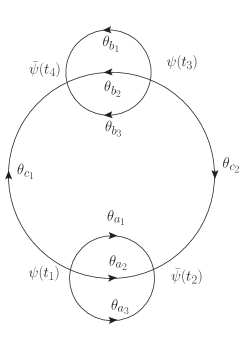
Figure 5: Direction of arrow is from $\psi$ to $\bar{\psi}$. The diagram is drawn for $q=4$.

The symmetry factor is calculated as follows. Any one of $q$ number of $\psi$’s of first $\psi$-vortex contracts with any one of $q$ number of $\bar{\psi}$’s of any one of two $\bar{\psi}$-vortex to give a factor of $2q^{2}$. Any one of $q$ number of $\psi$’s of second $\psi$-vortex contracts with any one of $q$ number of $\bar{\psi}$’s of remaining $\bar{\psi}$-vortex to give a factor of $q^{2}$. In large-N only non-suppressed diagram is obtained by joining $\psi$ to $\bar{\psi}$ (of same vortex) of same common colour. Choice of external propagator gives $q-1$ possibilities at each blob. Sign of the symmetry factor comes from noticing as there are two identical ’blobs’ sign of contraction of each blob cancel and overall sign is just because of contraction between two ’blobs’, it turns out to be -1. Contribution of symmetry factor at this order becomes

$$F_{4}=\frac{1}{4!}\ ^{4}C_{4/2}\ (-1)2[q^{2}(q-1)]^{2}I^{(4)},$$ (150)

where

$$I^{(4)}=\int\prod_{i=1}^{4}dt_{i}\ \left(\prod_{i=1}^{q-1}G_{0}(t_{12},\theta_{a_{i}})\right)\left(\prod_{i=1}^{q-1}G_{0}(t_{34},\theta_{b_{i}})\right)G_{0}(t_{32},\theta_{c_{2}})G_{0}(t_{14},\theta_{c_{1}}).$$ (151)

Where $\theta$s are holonomies on different propagators. Here time differences are not necessarily single valued and to satisfy the constraint

$$t_{12}+t_{23}+t_{34}+t_{41}=w\beta,$$

where $w=0,\pm 1,\pm 2$ (note that each $t_{ik}$ is in $(-\frac{\beta}{2},\frac{\beta}{2})$, and this restricts allowed values of $n$) we introduce dimensionless Lagrange multiplier integration

$$P\equiv\beta\int_{-\infty}^{+\infty}\frac{ds}{2\pi}e^{is(t_{12}+t_{23}+t_{34}+t_{41}-w\beta)}=\delta\left(\frac{t_{12}+t_{23}+t_{34}+t_{41}-w\beta}{\beta}\right).$$ (152)

In the scaling limit (assuming $m>0$), the propagator becomes

$$G_{0}(t)=e^{-(m+i\theta_{a})t}\theta(t)-xe^{-i\theta_{a}\beta}e^{-(m+i\theta_{a})t}\theta(t)-x^{1/2}e^{-m\beta/2}e^{-i\theta_{a}\beta}e^{-(m+i\theta_{a})t}\theta(-t).$$ (153)

This way of writing ensures in each of three parts of $G_{0}$ excluding explicit $x$ dependence integration over $-\frac{\beta}{2}$ to $\frac{\beta}{2}$ gives only positive powers of $x$. We will refer to these three parts of $G_{0}$ as $x^{0},x,x^{1/2}$ contributions.

In the scaling limit of interest $\ I^{(4)}$ can receive contribution from 5 different types of integration

$$I^{(4)}= \textit{$x^{0}$ everywhere}+\textit{$x^{1/2}$ on one of the outer ($\theta_{c_{1}},\theta_{c_{2}}$) lines}+\textit{$x^{1/2}$ on both of the outer lines}$$ (154)

$$+ \textit{$x$ on one of the outer lines}+\textit{$x$ on one of the inner lines ($\theta_{a_{1}},\theta_{a_{2}}\dots\theta_{a_{q-1}},\theta_{b_{1}},\theta_{b_{2}}\dots\theta_{b_{q-1}}$)}.$$

Note that choosing $x^{1/2}$ on one of the inner propagators will force choosing all the inner propagators in the same blob to be $x^{1/2}$ term due to unit step function. Therefore this choice is ignored in scaling limit calculation. Here we’ll present the calculation corresponding to the first one and mention results for others.

Consider $x^{1/2}$ on $\theta_{c_{1}}$ say, and on all others we choose x independent part of $G_{0}$. This ensures following time ordering for non-zero integrand $t_{12}>0,t_{32}>0,t_{34}>0,t_{41}>0$, with which only consistent values of $n$ are $0,1$. Contribution to $I^{(4)}$ becomes, omitting $\beta(-x^{1/2})e^{-i\theta_{c_{1}}\beta}e^{+i\theta_{c_{1}}w\beta}$ (for a contribution like $F_{0}$ we must have $n=0$ which is shown to be true below)

$$I^{(4)}\sim \ \beta(-x^{1/2})e^{-i\theta_{c_{1}}\beta}e^{+i\theta_{c_{1}}w\beta}\int\frac{ds}{2\pi}\ dt_{12}\ dt_{32}\ dt_{34}\ dt_{41}\ e^{-isw\beta}\ e^{-(m(q-1)-is)t_{12}}\times$$ (155)

$$\ \ \ \ \ \ \ \ \ \ \ \ \ \ \ \ \ \ \ \ \ \ \ \ \ \ \ \ \ \ \ \ \ \ \ \ \ \ \ \ \ \ \ \ \ \ \ \ \ \ e^{-(m(q-1)-is)t_{34}}\ e^{+(m+is)t_{41}-m\beta/2}e^{-(m+is)t_{32}}$$

$$= -\beta(-x^{1/2})e^{-i\theta_{c_{1}}\beta}e^{+i\theta_{c_{1}}w\beta}\int\frac{ds}{2\pi}\ \frac{(e^{is\beta/2}-x^{1/2})(x^{1/2}e^{-is\beta/2}-1)}{(s+i(q-1)m)^{2}(s-im)^{2}}e^{-isw\beta}+\mathcal{O}(x^{3/2}),$$

where we ignored higher order contributions in $x$. Simplifying the numerator gives 3 terms: $x$ independent piece that comes with a non-zero phase factor $e^{is\beta/2}$ (which will give a factor of $\beta$ upon integration because only $w=0$ will contribute), $x^{1/2}$ term that comes with no non-trivial phase (cannot give a $\beta$ upon integration), $x$ term drops out in scaling limit. Rest of the integration can be done easily choosing proper contour (semi-circle on upper or lower half plane as required by convergence) to ensure only $w=0$ term contributes to give the following result

$$\delta_{w,0}x^{1/2}\frac{2}{(qm)^{3}}\left(-1+\frac{q}{4}m\beta\right).$$ (156)

All other integrations can be performed similarly to give leading order contribution to free energy

$$F_{4}=\frac{1}{4!}\ ^{4}C_{4/2}\ 2q^{4}\frac{(q-1)^{2}}{q^{2}}m^{2}\beta^{2}\ N^{(q-1)^{2}}x\prod_{m=1}^{q-1}\rho^{1}_{m}+\mathcal{O}(\beta).$$ (157)

B.1.2 n melon graphs

Here a circle diagram with $n\geq 2$ blobs is considered and leading term in $\beta$ is calculated using methods demonstrated in previous sub-section.

Symmetry factor for the diagram in large N limit is

$$\frac{(-1)^{\frac{nq}{2}+n+1}}{(n!)^{2}}\ \ n!\ (q^{2})^{n}\ (n-1)!.$$ (158)

The leading order contribution in $\beta$ comes from two distinct choices - i) considering $x^{1/2}$ in any one of the $n$ external propagators (with holonomy $\theta_{a}$ say) with $x^{0}$ part of the free propagator in all others and ii) $x^{0}$ part of the free propagator in all propagators.

Contribution from the integral due to choice (i) is easily seen to be

$$-x^{1/2}|g|^{n}\ e^{-i\theta_{a}\beta+iw\theta_{a}\beta}\ \beta\int\frac{ds}{2\pi}\ e^{-i(w-\frac{1}{2})s\beta}\ \frac{1}{(-is+m(q-1))^{n}(is+m)^{n}}$$ (159)

$$=-2x\ |g|^{n}\ e^{-i\theta_{a}\beta}\frac{1}{(n-1)!}\left(\frac{\beta}{2mq}\right)^{n}\ \delta_{w,0},$$

where we have kept only highest power of $\beta$. Note that extra powers of beta $\beta^{n-1}$ came from the integration because of evaluation of residue around a pole of order $n$. This contribution is to be multiplied with a factor of $n$ due to freedom in choosing one external propagator on which $x^{1/2}$ is considered.

Now we turn to the choice (ii). In this case contribution to the integral is

$$|g|^{n}\ e^{iw\theta_{a}\beta}\ \beta\int\frac{ds}{2\pi}\ e^{-iws\beta}\ \frac{(1-x^{1/2}e^{-is\frac{\beta}{2}})^{n}}{(-is+m(q-1))^{n}(is+m)^{n}}$$ (160)

$$=2x\ |g|^{n}\ e^{-i\theta_{a}\beta}\frac{1}{(n-1)!}\left(\frac{\beta}{2mq}\right)^{n}\left(\frac{2^{n-1}}{n}-1\right)\ \delta_{w,1}.$$

As before we have kept only highest power of $\beta$. Note that this contribution vanishes for $n=2$.

After summing over the holonomies, and canceling loop N’s with that of scaling of $g$, contribution to free energy becomes

$$F_{2n}=2x\ N^{q-1}\left(\prod_{m=1}^{q-1}\rho^{1}_{m}\right)\ \frac{1}{(n-1)!}\left[\gamma(q)\ \frac{(-\beta)}{m}|J|^{2}\right]^{n}\left(2-\frac{2^{n-1}}{n}\right)+\mathcal{O}(\beta^{n-1}),$$ (161)

where

$$\gamma(q)=(-1)^{\frac{q}{2}(q-1)}\frac{q}{2}.$$ (162)

B.2 All powers of $\beta$ in a circle diagram

In this subsection we shall compute explicitly the integral involved in computing the contribution to the free energy in the scaling limit linear in $x=e^{-m\beta}$.

The free fermionic Green’s function at any finite temperature is given by,

$$\langle\psi(t)\bar{\psi}(0)\rangle \equiv G_{0}(t)$$ (163)

$$= \frac{1}{2}e^{-(m+i\alpha_{j})t}\Big{[}\textrm{sgn}(t)+\tanh\Big{(}\frac{\beta}{2}(m+i\alpha_{j})\Big{)}\Big{]}$$

$$= e^{-(m+i\alpha_{j})t}\Big{[}\theta(t)-xe^{-i\alpha_{j}\beta}\Big{]}\,,$$

where, $x=e^{-m\beta}<<1$ (scaling limit). Hence, one can also write the ‘reversed’ Green’s function at finite temperature as,

$$\langle\bar{\psi}(0)\psi(t)\rangle=G_{0}^{*}(-m) = \frac{1}{2}e^{(m+i\alpha_{j})t}\Big{[}\textrm{sgn}(t)-\tanh\Big{(}\frac{\beta}{2}(m+i\alpha_{j})\Big{)}\Big{]}.$$ (164)

Here $\alpha_{j}$ are holonomies, satisfying the following constraint

$$\sum\limits_{j=1}^{q}\alpha_{j}=0\,.$$ (165)

Now in the computation we use discrete representation of the delta function

$$\delta(t_{21}+t_{32}+t_{43}+t_{54}+t_{65}+\ .\ .\ .-t_{\overline{2n-1}\ \overline{2n}}+t_{1\ \overline{2n}})$$

$$={1\over 2\pi\beta}\sum\limits_{\omega=-\infty}^{\infty}e^{-2\pi i{\omega\over\beta}(t_{21}+t_{32}+t_{43}+t_{54}+t_{65}+\ .\ .\ .\ -t_{\overline{2n-1}\ \overline{2n}}+t_{1\ \overline{2n}}\ )}.$$ (166)

B.2.1 Evaluating the integral

Let us focus on the diagram which can be computed as using the integral,

$$I^{(2n)} = \tfrac{1}{2\pi\beta}\left(\tfrac{J}{4}\right)^{2n}\sum\limits_{\omega=-\infty}^{\infty}\left[\int_{-\beta/2}^{\beta/2}dt_{1}\ e^{-t_{1}\left(m+i\alpha_{q}\right)}e^{-2\pi i\frac{\omega}{\beta}t_{1}}\left(\textrm{sgn}(t_{1})+\tanh(\tfrac{m\beta+i\alpha_{q}\beta}{2})\right)\right.$$ (167)

$$\hskip 85.35826pt\left.\int_{-\beta/2}^{\beta/2}dt_{q}\ e^{t_{q}\left((q-1)m-i\alpha_{q}\right)}e^{-2\pi i\frac{\omega}{\beta}t_{q}}\left(A\ \textrm{sgn}(t_{q})-B)\right)\right]^{n}\,.$$

Here the first integral inside the sum is a single propagator while the second one represents the melon with $q-1$ propagatrs, where $A$ and $B$ are defined as

$$\prod\limits_{j=1}^{q-1}\left[\textrm{sgn}(t_{q})-\tanh(\tfrac{m\beta+i\alpha_{j}\beta}{2})\right]=(-1)^{q}\left(A\ \textrm{sgn}(t_{q})-B\right)\,.$$ (168)

We integrate over the time intervals of these propagators in (167) and since there are $n$ of them we raise it to the power $n$. However, we would also have to implement the constraint that the times add up to an integral of $\beta$. This is achieved by repesenting the delta function on a circle of length $\beta$ as an infinite sum. This contributes a factor of $e^{2\pi i\tfrac{\omega}{\beta}t_{i}}$ in each of the propagators as shown in (167).

Now we would like to focus on the integrals within the box brackets in (167)

$$F^{(2n)} = \sum\limits_{\omega=-\infty}^{\infty}\left[I^{(q)}_{\omega}\right]^{n}.$$ (169)

Upon integrating over $t_{1}$ and $t_{q}$ one finds that

$$I^{(q)}_{\omega} = \frac{f_{1}+f_{2}}{((q-1)m-i\alpha_{q}+z)(m+i\alpha_{q}-z)},\,\,\,z=-\frac{2\pi i\omega}{\beta}$$ (170)

Here $f_{1}$ consists of terms with $e^{\pm kz\beta}$ where $k\in{\mathbb{Z_{\rm even}}}$ while $f_{2}$ consists of terms $e^{\pm kz\beta/2}$ where $k\in{\mathbb{Z_{\rm odd}}}$. Its is evident that upon raising $I^{(q)}_{\omega}$ to $n$ one would have to evaluate sums in $z$ of the form

$$S_{1} = \sum\limits_{\omega=-\infty}^{\infty}\frac{e^{\pm kz\beta}}{(((q-1)m-i\alpha_{q}+z)(m+i\alpha_{q}-z))^{n}},\,k\in{\mathbb{Z_{\rm even}}}$$ (171)

$$S_{2} = \sum\limits_{\omega=-\infty}^{\infty}\frac{e^{\pm kz\beta/2}}{(((q-1)m-i\alpha_{q}+z)(m+i\alpha_{q}-z))^{n}},\,k\in{\mathbb{Z_{\rm odd}}}.$$ (172)

Since $z=-\tfrac{2\pi i\omega}{\beta}$ we see that these reduce to

$$S_{1} = \sum\limits_{\omega=-\infty}^{\infty}\frac{1}{(((q-1)m-i\alpha_{q}+z)(m+i\alpha_{q}-z))^{n}},$$ (173)

$$S_{2} = \sum\limits_{\omega=-\infty}^{\infty}\frac{e^{z\beta/2}}{(((q-1)m-i\alpha_{q}+z)(m+i\alpha_{q}-z))^{n}}.$$ (174)

We will use the technique of Matsubara summation to evaluate the above, where a weighting function is included to replace the sum by a contour integral. So, first let us evaluate $S_{1}$. With a weighting function $f(z)=\frac{1}{1-e^{z\beta}}$, one can replace the above summation with the following contour integral,

$$S_{1}=\oint\frac{dz}{(1-e^{z\beta})(((q-1)m-i\alpha_{q}+z)(m+i\alpha_{q}-z))^{n}}$$ (175)

Notice that the integrand has two poles at $z\equiv z_{a}=-(q-1)m+i\alpha_{q}$ and $z\equiv z_{b}=m+i\alpha_{q}$ and both are of $n$-th order. Using the residue theorem, one can evaluate the above integral as,

$$S_{1}=\lim_{z\to z_{a}}{1\over(n-1)!}\partial_{z}^{(n-1)}\frac{1}{(1-e^{z\beta})(z-z_{b})^{n}}+\lim_{z\to z_{b}}{1\over(n-1)!}\partial_{z}^{(n-1)}\frac{1}{(1-e^{z\beta})(z-z_{a})^{n}}$$ (176)

Now, it is very easy to verify that for any function $f(z)$,

$$\partial_{z}^{(n-1)}\Big{[}f(z)\frac{1}{(z-z_{a})^{n}}\Big{]}=\sum\limits_{k=0}^{n-1}(-1)^{k}\ {}^{(n-1)}C_{k}\ {(n+k-1)!\over(n-1)!}\ \frac{\partial_{z}^{(n-k-1)}f(z)}{(z-z_{a})^{n+k}}$$ (177)

In the present case, taking $f(z)={1\over(1-e^{\beta z})}$, one can evaluate

$$\partial_{z}^{(n)}\Big{[}\frac{1}{1-e^{\beta z}}\Big{]}={\beta^{n}e^{-\beta z}\over(e^{-\beta z}-1)^{n+1}}A(n)$$ (178)

where, $A(n)$ is the Eulerian polynomial in $e^{-\beta z}$, given by,

$$A(n)=\sum\limits_{m=0}^{n-1}\sum\limits_{k=0}^{m+1}(-1)^{k}\ {}^{n+1}C_{k}(m+1-k)^{n}\ e^{-\beta zm}$$ (179)

Using equation (178) and (179), one can easily obtain,

$$\partial_{z}^{(n-k-1)}f(z) = \partial_{z}^{(n-k-1)}\Big{[}\frac{1}{1-e^{\beta z}}\Big{]}$$ (180)

$$= {\beta^{n-k-1}\over(e^{-\beta z}-1)^{n-k}}\sum\limits_{m=0}^{n-k-2}\sum\limits_{l=0}^{m+1}(-1)^{l}\ {}^{n-k}C_{l}\ (m+1-l)^{n-k-1}e^{-\beta(m+1)z}$$

$$+ {1\over 1-e^{\beta z}}\delta_{n-k-1,0}$$

Finally Substituting equation (180) into equation (177), we have,

$$\partial_{z}^{(n-1)}\Big{[}{f(z)\over(z-z_{a})^{n}}\Big{]} = \partial_{z}^{(n-1)}\Big{[}\frac{1}{(1-e^{\beta z})(z-z_{a})^{n}}\Big{]}$$ (181)

$$= \sum\limits_{k=0}^{n-1}{(-1)^{k}\over(z-z_{a})^{n+k}}\ {}^{(n-1)}C_{k}\ {(n+k-1)!\over(n-1)!}\Big{[}{\beta^{n-k-1}\over(e^{-\beta z}-1)^{n-k}}\sum\limits_{m=0}^{n-k-2}\sum\limits_{l=0}^{m+1}(-1)^{l}$$

$$\ {}^{n-k}C_{l}\ (m+1-l)^{n-k-1}e^{-\beta(m+1)z}+{1\over 1-e^{\beta z}}\delta_{n-k-1,0}\Big{]}$$

Evaluating the above expression at both the poles $z=z_{a}$ and $z_{b}$, one can compute $S_{1}$ as expressed in equation (176).

Now let us discuss about evaluating the summation $S_{2}$ as given in equation (174). With a weighting function $f(z)=\frac{\ e^{\beta z/2}}{1-e^{\beta z}}$, one can replace the above summation with the following contour integral,

$$S_{2}=\oint\frac{e^{\beta z/2}dz}{(1-e^{\beta z})(((q-1)m-i\alpha_{q}+z)(m+i\alpha_{q}-z))^{n}}$$ (182)

Notice that we encounter the same $n$-th order poles in the contour integral as we had with $S_{1}$. The residue computation for evaluating this contour integral needs to evaluate the following term as before,

$$\partial_{z}^{(n)}f(z)=\partial_{z}^{(n)}\Big{[}\frac{e^{\beta z/2}}{1-e^{\beta z}}\Big{]}={\beta^{n}e^{-\beta z/2}\over 2^{n}(e^{-\beta z}-1)^{n+1}}B(n)$$ (183)

where, $B(n)$ is the Eulerian polynomial of type-B in $e^{-\beta z}$, given by,

$$B(n)=\sum\limits_{m=0}^{n}\sum\limits_{k=0}^{m}(-1)^{m-k}\ {}^{n+1}C_{m-k}(2k+1)^{n}\ e^{-\beta zm}$$ (184)

Finally, using equation (177), (183) and (184), one can obtain,

$$\partial_{z}^{(n-1)}\Big{[}\frac{f(z)}{(z-z_{a})^{n}}\Big{]} = \partial_{z}^{(n-1)}\Big{[}\frac{e^{\beta z/2}}{(1-e^{\beta z})(z-z_{a})^{n}}\Big{]}$$ (185)

$$= \sum\limits_{k=0}^{n-1}{(-1)^{k}\over(z-z_{a})^{n+k}}\ {}^{(n-1)}C_{k}\ {(n+k-1)!\over(n-1)!}{\beta^{n-k-1}\over 2^{n-k-1}(e^{-\beta z}-1)^{n-k}}$$

$$\sum\limits_{m=0}^{n-k-1}\sum\limits_{l=0}^{m}(-1)^{m-l}\ {}^{n-k}C_{m-l}\ (2l+1)^{n-k-1}e^{-(2m+1)\beta z/2}$$

Now using the above equation one can compute the residue and hence the integral (182). This finishes the computation of $S_{2}$ as given in equation (174).

One finds that $S_{1}$ depends only linearly on $x=e^{-m\beta}$ while $S_{2}$ depends as $\sqrt{x}$. Further noting that the difference in $A$ and $B$ in (168) behaves as $A-B={\mathcal{O}}(x^{q-1})$ we find that $f_{1}=(A-B){\mathcal{O}}(x^{\tfrac{-q}{2}+1})={\mathcal{O}}(x^{q/2})$ and $f_{2}=(A-B){\mathcal{O}}(x^{\tfrac{-q+1}{2}})={\mathcal{O}}(x^{\tfrac{q}{2}-1})$. Therefore in the scaling limit one can take $A=B=2^{q-2}\left(1-x\sum\limits_{j=1}^{q-1}e^{-i\beta\alpha_{j}}\right)$.

Therefore evaluating $(f_{1}+f_{2})^{N}\approx F_{1}+F_{2}$ in the scaling limit- where once again $F_{1}$ consists of terms with $e^{\pm kz\beta}$ where $k\in{\mathbb{Z}}$ while $F_{2}$ consists of terms $e^{\pm kz\beta/2}$ where $k\in{\mathbb{Z_{\rm odd}}}$, $F^{(n)}=S_{1}\bar{F}_{1}+S_{2}\bar{F}_{2}$. Here $\bar{F}_{1,2}=F_{1,2}(z=0)$.

The fact that only these two type of summations contribute for any integer value of $k$, makes it easier to evaluate equation (167) in the scaling limit as,

$$I^{(2n)}\!\!\! = \!\!\!J^{2n}\sum\limits_{k=0}^{n-2}\frac{2^{(q-1)n}x\beta^{n-k}}{(mq)^{n+k}\Gamma(n)^{2}}(2^{n}-2^{2+k}n)(^{n-1}C_{k})\Gamma(n+k)\prod_{m=1}^{q-1}\rho^{1}_{m}$$ (186)

which can be re-written as

$$I^{(2n)}\!\!\! = \!\!\!\left(\frac{J^{2}\beta}{mq}\right)^{n}\,\,\sum\limits_{k=0}^{n-2}\left(\frac{J^{2}}{m^{2}}\right)^{k}\left(\frac{m}{qJ^{2}\beta}\right)^{k}\frac{2^{(q-1)n}x}{\Gamma(n)^{2}}(2^{n}-2^{2+k}n)(^{n-1}C_{k})\Gamma(n+k)\prod_{m=1}^{q-1}\rho^{1}_{m}$$ (188)

$$\hskip 312.9803pt+{\mathcal{O}(\beta)}$$

or equivalently keep all orders in $\beta$ as

$$I^{(2n)}={J^{2n}\over m^{2n}q^{n}}\frac{(-1)^{q(n-1)}}{(n-1)!}\bigg{[} \frac{(2n-2)!}{(n-1)!\ q^{n-1}}m\beta\bigg{(}1-n\Big{(}q-2n+3\Big{)}\bigg{)}$$

$$+\sum_{k=0}^{n-2}\frac{(n+k-1)!}{k!(n-k-1)!\ q^{k}}(1-2^{k+2-n}n)(m\beta)^{n-k}\ \bigg{]}\ x\left(\prod_{m=1}^{q-1}\rho^{1}_{m}\right).$$

This multiplied with (158)$\times N^{q-1}$ gives contribution of a circle diagram with n melons.

B.3 Evaluating the subleading correction

We end this appendix by presenting a technical result which we do not use in the main text of the paper, but record here anyway, just in case this result finds application subsequent work.

The technical result we report here is the evaluation of the Feynman integral for diagram Fig. (6) (the figure is drawn for $q=4$ but we present the evaluation in general), which is one of the diagrams that would contribute to the generalization of the results presented in this paper to subleading orders in $\frac{1}{\beta}$. We present the result for the Feynman diagram ignoring the symmetry factor (which can easily be independently evaluated). We evaluate the diagram of Fig. (6) as follows. In order to get the integrand of the diagram we first multiply together all the propgators that make it up, keeping careful track of holonomy factors and making use of the fact that holonomies at any interaction vertex sum to zero. The integrand is the term in the big square bracket in (195) with $\epsilon_{1}$ and $\epsilon_{2}$ temporarily set to zero. The first two lines on the RHS of (195) are the $n-2$ factors on the in the diagram Fig.(7).

The next four lines on the RHS of (195) represent the second factor in Fig.(7). Lines 3-6 on the RHS of (195) are the remaing factors (the propagators outside the square bracket) in Fig.(7).

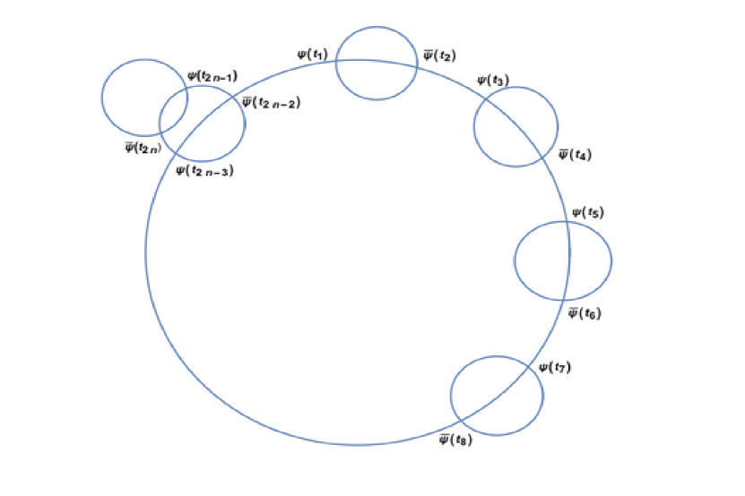
Figure 6: subleading diagram

$$I^{(2n-2)} = \left(\tfrac{1}{2\pi\beta}\right)^{2}\sum\limits_{\omega_{1},\omega_{2}=-\infty}^{\infty}\left[\left(\int_{-\beta/2}^{\beta/2}dt_{1}e^{-(m+i\alpha_{1}+i\tfrac{\epsilon_{1}}{\beta})t_{1}}\left({\rm sgn}(t_{1})+\tanh(\tfrac{m\beta+i\alpha_{1}\beta}{2})\right)\right.\right.$$ (195)

$$\left.\hskip 99.58464pt\int_{-\beta/2}^{\beta/2}dt_{2}e^{((q-1)m-i\alpha_{1}-i\tfrac{\epsilon_{1}}{\beta})t_{2}}\left({\rm sgn}(t_{2})A_{1}-B_{1}\right)\right)^{n-2}$$

$$\hskip 99.58464pt\int_{-\beta/2}^{\beta/2}dt_{1}e^{-(m+i\alpha_{1}+i\tfrac{\epsilon_{1}}{\beta})t_{1}}\left({\rm sgn}(t_{1})+\tanh(\tfrac{m\beta+i\alpha_{1}\beta}{2})\right)$$

$$\hskip 99.58464pt\left(\int_{-\beta/2}^{\beta/2}dt_{3}e^{(m+i\alpha_{2}+i\tfrac{\epsilon_{2}}{\beta})t_{3}}\left({\rm sgn}(t_{3})-\tanh(\tfrac{m\beta+i\alpha_{2}\beta}{2})\right)\right)^{2}$$

$$\hskip 99.58464pt\int_{-\beta/2}^{\beta/2}dt_{4}e^{((q-2)m-i(\alpha_{1}+\alpha_{2})-i\tfrac{(\epsilon_{1}+\epsilon_{2})}{\beta})t_{4}}\left({\rm sgn}(t_{4})A_{1,2}-B_{1,2}\right)$$

$$\left.\hskip 99.58464pt\int_{-\beta/2}^{\beta/2}dt_{5}e^{(-(q-1)m+i\alpha_{2}+i\tfrac{\epsilon_{2}}{\beta})t_{5}}\left({\rm sgn}(t_{5})A_{2}+B_{2}\right)\right]$$

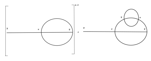
Figure 7: parts of subleading diagram

After evaluating the integrand we need to perform the integrals. Roughly speaking we must integrate all propagator lengths in the integrand above from $-\frac{\beta}{2}$ to $\frac{\beta}{2}$. However we need to do this subject to the constraint that as we go round either of the two circles in the diagram Fig.(6) we come back to the same time as we started out, modulo $\beta$. This is where the parameters $\epsilon_{1}$ and $\epsilon_{2}$ in (195) come in. $\epsilon_{1}$ couples to the sum of lengths of propagators in units of $\beta$ around the big circle in Fig.(6), while $\epsilon_{2}$ multiplies the sum of the lengths of all the propagators as we go around the small circle - again in units of $\beta$ in Fig.(6). The constraint that these lengths evaluate to an integral multiple of $\beta$ can then be implemented by setting $\epsilon_{1,2}=2\pi\omega_{1,2}$ and then summing $\omega_{i}$ over all integral values, as we have done in (195).

In order to proceed we perform the time integrals in an unconstrained manner. The result can be rearranged (according to its $\omega_{i}$ dependence) as a sum of four types of terms.

1. Terms containing $e^{k(z_{1}+z_{2})\beta}$ where $k\in{\mathbb{Z}}$

2. those with $e^{kz_{1}\beta/2}$ where $k\in{\mathbb{Z}_{\rm odd}}$

3. with $e^{kz_{2}\beta/2}$ where $k\in{\mathbb{Z}_{\rm odd}}$

4. and $e^{k(z_{1}+z_{2})\beta/2}$ where $k\in{\mathbb{Z}_{\rm odd}}$;

where $z_{i}=-\frac{2\pi i}{\beta}\omega_{i}.$

We deal with these four classes of terms spearately; for each class we explicitly perform the sum over $\omega_{i}$ (by reducing it to a contour integral as in the previous subsection) and expand the resultant expression in a Taylor series in $x$ (again as in the previous subsection), keep only the terms that are linear in $x$. Combining together the results from each of the four classes we obtain our final result

$$I^{(2n-2)}\!\! = \!\!-\left(\frac{J^{2}\beta}{mq}\right)^{n}\sum\limits_{k=0}^{n-4}\frac{x(q-1)}{(mq\beta)^{k+1}}\frac{2^{(q-1)n}(2^{n}+(n-1)2^{3+k})(2n+k-2)\Gamma(n+k-1)}{\Gamma(n-k-1)\Gamma(n)\Gamma(1+k)}\prod_{m=1}^{q-1}\rho^{1}_{m}$$ (197)

$$\hskip 312.9803pt+{\mathcal{O}(\beta^{2})}$$

(the terms ${\mathcal{O}(\beta^{2})}$ that we have omitted to list in (197) are the terms with $k=n-3$ and $k=n-2$ which exist in the final answer but the values of whose coefficients do not follow the uniform rule of the other terms).

Note that (197) scales like $\frac{1}{\beta}$ in coordinated large $\beta$ small $J$ limit in which $J^{2}\beta$ is held fixed.

Appendix C The holonomy effective action from the sigma model

In this section we ask the following question: what is the contribution to $S_{\text{eff}}(U)$ - the effective action for holonomies - resulting from integrating out the new light degrees of freedom discovered in the massless tensor model in early sections in this paper? In the bulk of this section we address this question at the technical level. At the end of the section we turn to a quick discussion of its physical import.

Turning on holonomy is equivalent to putting appropriate boundary condition on fermion fields. This translates into boundary condition on $V_{l}$, given by $V_{l}(-\frac{\beta}{2})=UV_{l}(+\frac{\beta}{2})$, $U\in O(N)$. This boundary condition is equivalent to the computation of the partition function

$$Z=e^{-S_{\text{eff}}(U)}=\operatorname{Tr}e^{-\beta H}{\hat{U}},$$ (198)

where $H$ is the Hamiltonian of the quantum mechanical system (3) and $U$ is the quantum mechanical operator that implements left rotations on the sigma model by the $O(N)^{q-1}$ group rotation $U$. The partition function (2) is the product of $q-1$ factors, associated with the sigma models on the $q-1$ gauge groups. It follows that the effective action $S_{\text{eff}}(U)$ that follows from this computation takes the form

$$S_{\text{eff}}(U)=\sum_{i}S(U_{i}).$$ (199)

In the rest of this section we compute the functions $S(U_{i})$

Let us first note that the Hilbert $H$ space on which any one of the factors of $q-1$ distinct factors the sigma model (3) acts is given as follows. The Hamiltonian acts on the Hilbert space $H$

$$H=\sum_{R_{i}}{\tilde{R}_{i}}\otimes{\tilde{R}_{i}}.$$ (200)

The sum $R_{i}$ runs over all genuine (as opposed to spinorial) representations of $O(N)$. ${\tilde{R}_{i}}$ denotes the vector space on which $O(N)$ acts in the $i^{th}$ representation. The space ${\tilde{R}_{i}}\otimes{\tilde{R}_{i}}$ transforms in the representation $R_{i}\times R_{i}$ under $O(N)_{L}\times O(N)_{R}$; the operator ${\hat{U}}$ acts as an $O(N)$ rotation on the first ${\tilde{R}_{i}}$ but as identity on the second ${\tilde{R}_{i}}$. The Hamiltonian corresponding to action (3) is diagonal under the decomposition (200); the energy of the $i^{th}$ factor of the Hilbert space is $\frac{JC_{2}(R_{i})}{2{\mathcal{A}}N^{q-2}}$.

Representations of $O(N)$ are conveniently labeled by the highest weights $(h_{1},h_{2},h_{3}\ldots)$, the charges under rotations in mutually orthogonal two planes. Let $h=\sum_{i}h_{i}$. At leading order in the large $N$ limit the dimensionality of the representation $R_{i}$ depends only on $h$ and is given by

$$d(R_{i})=\frac{N^{h}}{h!}.$$

Moreover the Casimir $C_{2}(R_{i})$ of representations of $O(N)$ also depends only on $h$ at leading order in the large $N$ limit and is given by

$$C_{2}(R_{i})=Nh.$$

Let $\chi_{R_{i}}(U)$ denote the character in the $R_{i}$ representation of $O(N)$ and let

$$\chi_{n}(U)=\sum_{R_{i}\in{\hat{n}}}\chi_{R_{i}}(U),$$ (201)

where ${\hat{n}}$ denotes the collection of all representations of $O(N)$ with $h=n$. In other words $\chi_{n}(U)$ is the sum over the characters of all representations with $h=n$.

Note that all representations with $h=n$ can be constructed - and can be constructed exactly once - from the direct products of $n$ vectors of $O(N)$ (this is true when $N\gg n$ as we assume). Let $P_{n}$ denote the projector onto representations with $h=n$

$$P_{n}\left[f(U))\right]=\int dU^{\prime}\sum_{R_{i}\in{\hat{n}}}\chi_{R_{i}}(U)\chi^{*}_{R_{i}}(U^{\prime})f(U^{\prime}).$$ (202)

It follows that

$$\chi_{n}(U)=P_{n}\left[(\operatorname{Tr}U)^{n}\right].$$ (203)

where $U$ on the RHS of (203) represents the group element in the vector representation of $O(N)$.

Finally we define

$$z=e^{-\frac{J}{2AN^{q-3}}}.$$ (204)

It follows immediately from all the facts and definitions presented above that

$$e^{-S(U_{i})}=\sum_{n=0}^{\infty}\frac{(zN)^{n}}{n!}\chi_{n}(U_{i}).$$ (205)

Using (203), (205) can be rewritten in the (perhaps deceptively) elegant form

$$e^{-S(U_{i})}=P_{z\partial_{z}}e^{Nz\operatorname{Tr}(U_{i})}.$$ (206)

Note that

$$\int dUe^{-S(U)}=1.$$ (207)

This is an immediate consequence of the fact that the vacuum is the only representation in the spectrum of the group sigma model that is a singlet under $O(N)_{L}$. It follows that the partition function generated by $S(U)$ by itself is trivial. However $S(U)$ is only one piece of the effective action for $U$ in the massless tensor model (1); we get other contributions to the effective action by integrating out the fermionic fields themselves (as was explicitly done earlier in this paper for the case of massive fermions). When put together with other contributions the effective action (206) could have a significant impact on the partition function, especially at temperatures scaled to ensure that the matter contribution to the effective action - like the contribution of the sigma model considered in this section - is of order $N^{2}$.

References

- (1) S. Sachdev, Holographic metals and the fractionalized Fermi liquid, Phys. Rev. Lett. 105 (2010) 151602, [1006.3794].
-
(2)
A. Kitaev, “A simple model of quantum holography”,
http://online.kitp.ucsb.edu/online/entangled15/kitaev/
http://online.kitp.ucsb.edu/online/entangled15/kitaev2/
“Talks at KITP, April 7, 2015 and May 27, 2015.” - (3) J. Maldacena and D. Stanford, Remarks on the Sachdev-Ye-Kitaev model, Phys. Rev. D94 (2016) 106002, [1604.07818].
- (4) A. Almheiri and J. Polchinski, Models of AdS2 backreaction and holography, JHEP 11 (2015) 014, [1402.6334].
- (5) K. Jensen, Chaos in AdS2 Holography, Phys. Rev. Lett. 117 (2016) 111601, [1605.06098].
- (6) J. Maldacena, D. Stanford and Z. Yang, Conformal symmetry and its breaking in two dimensional Nearly Anti-de-Sitter space, PTEP 2016 (2016) 12C104, [1606.01857].
- (7) G. Mandal, P. Nayak and S. R. Wadia, Coadjoint orbit action of Virasoro group and two-dimensional quantum gravity dual to SYK/tensor models, 1702.04266.
- (8) D. J. Gross and V. Rosenhaus, The Bulk Dual of SYK: Cubic Couplings, JHEP 05 (2017) 092, [1702.08016].
- (9) S. Forste and I. Golla, Nearly AdS2 sugra and the super-Schwarzian, Phys. Lett. B771 (2017) 157–161, [1703.10969].
- (10) S. R. Das, A. Jevicki and K. Suzuki, Three Dimensional View of the SYK/AdS Duality, 1704.07208.
- (11) A. M. García-García and J. J. M. Verbaarschot, Spectral and thermodynamic properties of the Sachdev-Ye-Kitaev model, Phys. Rev. D94 (2016) 126010, [1610.03816].
- (12) J. S. Cotler, G. Gur-Ari, M. Hanada, J. Polchinski, P. Saad, S. H. Shenker et al., Black Holes and Random Matrices, JHEP 05 (2017) 118, [1611.04650].
- (13) A. M. García-García and J. J. M. Verbaarschot, Analytical Spectral Density of the Sachdev-Ye-Kitaev Model at finite N, 1701.06593.
- (14) D. Stanford and E. Witten, Fermionic Localization of the Schwarzian Theory, 1703.04612.
- (15) V. V. Belokurov and E. T. Shavgulidze, The Exact Solution of the Schwarzian Theory, 1705.02405.
- (16) E. Witten, An SYK-Like Model Without Disorder, 1610.09758.
- (17) I. R. Klebanov and G. Tarnopolsky, Uncolored Random Tensors, Melon Diagrams, and the SYK Models, 1611.08915.
- (18) I. R. Klebanov and G. Tarnopolsky, On Large Limit of Symmetric Traceless Tensor Models, 1706.00839.
- (19) R. Gurau, Colored Group Field Theory, Commun. Math. Phys. 304 (2011) 69–93, [0907.2582].
- (20) R. Gurau, The 1/N expansion of colored tensor models, Annales Henri Poincare 12 (2011) 829–847, [1011.2726].
- (21) R. Gurau and V. Rivasseau, The 1/N expansion of colored tensor models in arbitrary dimension, Europhys. Lett. 95 (2011) 50004, [1101.4182].
- (22) R. Gurau, The complete 1/N expansion of colored tensor models in arbitrary dimension, Annales Henri Poincare 13 (2012) 399–423, [1102.5759].
- (23) V. Bonzom, R. Gurau, A. Riello and V. Rivasseau, Critical behavior of colored tensor models in the large N limit, Nucl. Phys. B853 (2011) 174–195, [1105.3122].
- (24) R. Gurau and J. P. Ryan, Colored Tensor Models - a review, SIGMA 8 (2012) 020, [1109.4812].
- (25) P. Narayan and J. Yoon, SYK-like Tensor Models on the Lattice, 1705.01554.
- (26) J. Yoon, SYK Models and SYK-like Tensor Models with Global Symmetry, 1707.01740.
- (27) S. Dartois, H. Erbin and S. Mondal, Conformality of corrections in SYK-like models, 1706.00412.
- (28) T. Nishinaka and S. Terashima, A Note on Sachdev-Ye-Kitaev Like Model without Random Coupling, 1611.10290.
- (29) C. Peng, M. Spradlin and A. Volovich, A Supersymmetric SYK-like Tensor Model, JHEP 05 (2017) 062, [1612.03851].
- (30) C. Krishnan, S. Sanyal and P. N. Bala Subramanian, Quantum and Holographic Tensor Models, JHEP 03 (2017) 056, [1612.06330].
- (31) F. Ferrari, The Large D Limit of Planar Diagrams, 1701.01171.
- (32) R. Gurau, Quenched equals annealed at leading order in the colored SYK model, 1702.04228.
- (33) V. Bonzom, L. Lionni and A. Tanasa, Diagrammatics of a colored SYK model and of an SYK-like tensor model, leading and next-to-leading orders, J. Math. Phys. 58 (2017) 052301, [1702.06944].
- (34) C. Krishnan, K. V. P. Kumar and S. Sanyal, Random Matrices and Holographic Tensor Models, JHEP 06 (2017) 036, [1703.08155].
- (35) S. Chaudhuri, V. I. Giraldo-Rivera, A. Joseph, R. Loganayagam and J. , Abelian Tensor Models on the Lattice, 1705.01930.
- (36) T. Azeyanagi, F. Ferrari and F. I. Schaposnik Massolo, Phase Diagram of Planar Matrix Quantum Mechanics, Tensor and SYK Models, 1707.03431.
- (37) S. Giombi, I. R. Klebanov and G. Tarnopolsky, Bosonic Tensor Models at Large and Small , 1707.03866.
- (38) S. Sachdev, K. Jensen, Y. Gu, A. Georges, W. Fu and R. A. Davison, Thermoelectric transport in disordered metals without quasiparticles: the Sachdev-Ye-Kitaev models and holography, 1612.00849v2.
- (39) O. Aharony, J. Marsano, S. Minwalla, K. Papadodimas and M. Van Raamsdonk, The Hagedorn - deconfinement phase transition in weakly coupled large N gauge theories, Adv. Theor. Math. Phys. 8 (2004) 603–696, [hep-th/0310285].
- (40) E. Witten, Anti-de Sitter Space, Thermal Phase Transition, And Confinement In Gauge Theories, 9803131v2.
- (41) O. Aharony, J. Marsano, S. Minwalla, K. Papadodimas and M. Van Raamsdonk, A First order deconfinement transition in large N Yang-Mills theory on a small S**3, Phys. Rev. D71 (2005) 125018, [hep-th/0502149].
- (42) J. M. Maldacena, Eternal black holes in anti-de Sitter, JHEP 04 (2003) 021, [hep-th/0106112].
- (43) K. Bulycheva, I. R. Klebanov, A. Milekhin and G. Tarnopolsky, Spectra of Operators in Large Tensor Models, 1707.09347.
- (44) C. Krishnan and K. V. P. Kumar, Towards a Finite- Hologram, 1706.05364.
- (45) D. J. Gross and E. Witten, Possible Third Order Phase Transition in the Large N Lattice Gauge Theory, Phys. Rev. D21 (1980) 446–453.
- (46) S. R. Wadia, A Study of U(N) Lattice Gauge Theory in 2-dimensions, 1212.2906.
- (47) S. R. Wadia, = Infinity Phase Transition in a Class of Exactly Soluble Model Lattice Gauge Theories, Phys. Lett. B93 (1980) 403–410.
- (48) M. R. Gaberdiel and R. Gopakumar, Minimal Model Holography, J. Phys. A46 (2013) 214002, [1207.6697].
- (49) C.-M. Chang, S. Minwalla, T. Sharma and X. Yin, ABJ Triality: from Higher Spin Fields to Strings, J. Phys. A46 (2013) 214009, [1207.4485].