Compressive Sensing with Cross-Validation and Stop-Sampling
for Sparse Polynomial Chaos Expansions

Abstract

Compressive sensing is a powerful technique for recovering sparse solutions of underdetermined linear systems, which is often encountered in uncertainty quantification analysis of expensive and high-dimensional physical models. We perform numerical investigations employing several compressive sensing solvers that target the unconstrained LASSO formulation, with a focus on linear systems that arise in the construction of polynomial chaos expansions. With core solvers of l1  ls, SpaRSA, CGIST, FPC  AS, and ADMM, we develop techniques to mitigate overfitting through an automated selection of regularization constant based on cross-validation, and a heuristic strategy to guide the stop-sampling decision. Practical recommendations on parameter settings for these techniques are provided and discussed. The overall method is applied to a series of numerical examples of increasing complexity, including large eddy simulations of supersonic turbulent jet-in-crossflow involving a 24-dimensional input. Through empirical phase-transition diagrams and convergence plots, we illustrate sparse recovery performance under structures induced by polynomial chaos, accuracy and computational tradeoffs between polynomial bases of different degrees, and practicability of conducting compressive sensing for a realistic, high-dimensional physical application. Across test cases studied in this paper, we find ADMM to have demonstrated empirical advantages through consistent lower errors and faster computational times.

1 Introduction

Compressive sensing (CS) started as a breakthrough technique in signal processing around a decade ago [7, 10]. It has since been broadly employed to recover sparse solutions of underdetermined linear systems where the number of unknowns exceeds the number of data measurements. Such a system has an infinite number of solutions, and CS seeks the sparsest solution—that is, solution with the fewest number of non-zero components, minimizing its $\ell_{0}$-norm. This $\ell_{0}$-minimization is an NP-hard problem, however, and a simpler convex relaxation minimizing the $\ell_{1}$-norm is often used as an approximation, which can be shown to reach the $\ell_{0}$ solution under certain conditions [11]. Several variants of $\ell_{1}$-sparse recovery are thus frequently studied:

(BP) $$\min_{x}\left\|\,x\,\right\|_{1} Ax=y,$$ subject to (1)

(BPDN) $$\min_{x}\left\|\,x\,\right\|_{1} \left\|\,Ax-y\,\right\|_{2}^{2}<\epsilon,$$ subject to (2)

(LASSO) $$\min_{x}\left\|\,Ax-y\,\right\|_{2}^{2} \left\|\,x\,\right\|_{1}<\tau,$$ subject to (3)

(uLASSO) $$\min_{x}\left\|\,Ax-y\,\right\|_{2}^{2}+\lambda\left\|\,x\,\right\|_{1},$$ (4)

where $A\in\mathbb{R}^{m\times n}$ ($m$ is the number of data samples, and $n$ the number of basis functions), $x\in\mathbb{R}^{n}$, $y\in\mathbb{R}^{m}$, $\epsilon>0$ and $\tau>0$ are scalar tolerances, and $\lambda\geq 0$ is a scalar regularization parameter. Equation 1 (BP) is known as the basis pursuit problem; Equation 2 (BPDN) is the basis pursuit denoising; Equation 3 (LASSO) is the (original) least absolute shrinkage and selection operator; and Equation 4 (uLASSO) is the unconstrained LASSO (also known as the Lagrangian BPDN, or simply the $\ell_{1}$-regularized least squares). These variants are closely related to each other, and in fact Equations 2, 3 and 4 can be shown to arrive at the same solution for appropriate choices of $\epsilon$, $\tau$, and $\lambda$, although their relationships are difficult to determine a priori [45].

The connections among these optimization statements do not imply they are equally easy or difficult to solve, and different algorithms and solvers have been developed to specifically target each form. For example, least angle regression (LARS) [14] accommodates Equation 3 by iteratively expanding a basis following an equiangular direction of the residual; primal-dual interior point methods (e.g., [8]) can be used to solve Equations 1 and 2 by reformulating them as “perturbed” linear programs; $\ell_{1}$-magic [7] recasts Equation 2 as a second-order cone program and leverages efficient log-barrier optimization; and many more. Greedy algorithms such as orthogonal matching pursuit (OMP) [9] rely on heuristics, do not target any particular optimization formulation, and have been demonstrated to work very well in many situations.

We focus on the uLASSO problem Equation 4. This unconstrained setup is of significant interest, being related to convex quadratic programming, for which many algorithms and solvers have already been developed [45]. The uLASSO problem also shares a close connection with Bayesian statistics, where the minimizer can be interpreted to be the posterior mode corresponding to a likelihood encompassing additive Gaussian noise on a linear model and a log-prior with the $\ell_{1}$ form. Bayesian compressive sensing (BCS) methods [30, 2] take advantage of this perspective, and leverage Bayesian inference methods to explore the posterior distribution that can be useful in assessing solution robustness around the mode. We do not investigate BCS in this paper, and focus only on non-Bayesian approaches for the time being. Various algorithms have been developed to directly target Equation 4 relying on different mathematical principles, and they may perform differently in practice depending on the problem structure. It is thus valuable to investigate and compare them under problems and scenarios we are interested in. In this study, we perform numerical experiments using several off-the-shelf solvers: l1  ls [32, 33], sparse reconstruction by separable approximation (SpaRSA) [49, 48], conjugate gradient iterative shrinkage/thresholding (CGIST) [21, 22], fixed point continuation with active set (FPC  AS) [47, 52], and alternating direction method of multipliers (ADMM) [5, 6].

The l1  ls algorithm transforms Equation 4 to a convex quadratic problem with linear inequality constraints. The resulting formulation is solved using a primal interior-point method with logarithmic barrier functions while invoking iterations of conjugate gradient (CG) or truncated Newton. SpaRSA takes advantage of a sequence of related optimization subproblems with quadratic terms and diagonal Hessians, where their special structure leads to rapid solutions and convergence. CGIST is based on forward-backward splitting with adaptive step size and parallel tangent (partan) CG acceleration. The eventual stabilization of the active set from the splitting updates renders the problem quadratic, at which point partan CG produces convergence in a finite number of steps. FPC  AS alternates between two stages: establishing a working index set using iterative shrinkage and line search, and solving a smooth subproblem defined by the (usually lower dimensional) working index set through a second-order method such as CG. Finally, ADMM combines techniques from dual descent and the method of multipliers, and naturally decomposes the $\ell_{1}$ term from $\ell_{2}$, requiring only iterations of small local subproblems where analytical updates can be obtained from ridge regression and soft thresholding formulas.

We further target the use of CS for polynomial chaos expansion (PCE) construction. PCE is a spectral expansion for random variables, and offers an inexpensive surrogate modeling alternative for representing probabilistic input-output relationships. It is a valuable tool for enabling computationally feasible uncertainty quantification (UQ) analysis of expensive engineering and science applications (e.g., [20, 37, 50, 34]). The number of PCE basis terms grows drastically with the parameter dimension and polynomial order, while the number of available model evaluations are often few and limited due to high simulation costs. Consequently, constructing sparse PCEs is both desirable and necessary especially for high-dimensional problems, and research efforts are growing across several fronts to tackle this challenge.

In general, sampling efficiency is a major topic of interest, mainly due to the potential computational expense of each isolated model evaluation. Rauhut and Ward [41] demonstrated advantages of Chebyshev sampling for Legendre PCEs while Hampton and Doostan [24] proposed coherence-optimal sampling for a general orthonormal basis using Markov chain Monte Carlo. Recently, Jakeman, Narayan, and Zhou [29] illustrated the advantages of sampling with respect to a weighted equilibrium measure followed by solving a preconditioned $\ell_{1}$-minimization problem. Fajraoui, Marelli, and Sudret [17] also adopted linear optimal experimental design practice to iteratively select samples maximizing metrics based on the Fisher information matrix. Another strategy involves tailoring the objective function directly, such as using weighted $\ell_{1}$-minimization [40] for more targeted recovery of PCE coefficients that are often observed to decay in physical phenomena. Eldred et al. [15] described a different perspective that combined CS in a multifidelity framework, which can achieve high overall computation efficiency by trading off between accuracy and cost across different models. All these approaches, however, maintain a static set of basis functions (i.e., regressors or features). A promising avenue of advancement involves adapting the basis dictionary iteratively based on specified objectives. For example, works by Sargsyan et al. [42] and Jakeman, Eldred, and Sargsyan et al. [28] incorporated the concept of “front-tracking”, where the basis set is iteratively pruned and enriched according to criteria reflecting the importance of each term. In our study, we investigate different numerical aspects of several CS solvers under standard sampling strategies and fixed basis sets.

By promoting sparsity, CS is designed to reduce overfitting. An overfit solution is observed when the error on the training set (i.e., data used to define the underdetermined linear system) is very different (much smaller) than error on a separate validation set, and the use of a different training set could lead to entirely different results. Such a solution has poor predictive capability and is thus unreliable. However, CS is not always successful in preventing overfitting, such as when emphases of fitting the data and regularization are not properly balanced, or if there is simply too little data. In the context of sparse PCE fitting, Blatman and Sudret [4] developed a LARS-based algorithm combined with a model selection score utilizing leave-one-out cross-validation, which helped both to avoid overfitting and to inform the sampling strategy. In this paper, we also explore approaches for addressing these challenges while focusing on solvers aimed at the uLASSO problem. Specifically, we use techniques to help improve the mitigation of overfitting on two levels. First, for a given set of data points, we employ cross-validation (CV) error to reflect the degree of overfitting of solutions obtained under different $\lambda$, and choose the solution that minimizes CV error. However, when sample size is too small, then the solutions could be overfit no matter what $\lambda$ is used. A minimally-informative sample size is problem-dependent, difficult to determine a priori, and may be challenging to even define and detect in real applications where noise and modeling errors are large. We provide a practical procedure to use information from existing data to help guide decisions as to whether additional samples would be worthwhile to obtain—i.e., a stop-sampling strategy. While previous work focused on rules based on the stabilization of solution versus sample size [36], we take a goal-oriented approach to target overfitting, and devise a strategy using heuristics based on CV error levels and their rates of improvement.

The main objectives and contributions of this paper are as follows.

• We conduct numerical investigations to compare several CS solvers that target the uLASSO problem Equation 4. The scope of study involves using solver implementations from the algorithm authors, and focusing on assessments of linear systems that emerge from PCE constructions. The solvers employ their default parameter settings.

• We develop techniques to help mitigate overfitting through

  • an automated selection of regularization constant $\lambda$ based on CV error and

  • a heuristic strategy to guide the stop-sampling decision.

• We demonstrate the overall methodology in a realistic engineering application, where a 24-dimensional PCE is constructed with expensive large eddy simulations of supersonic turbulent jet-in-crossflow (JXF). We examine performance in terms of recovery error and timing.

This paper is outlined as follows. Section 2 describes the numerical methodology used to solve the overall CS problem. Section 3 provides a brief introduction to PCE, which is the main form of linear systems we focus on. Numerical results on different cases of increasing complexity are presented in section 4. The paper then ends with conclusions and future work in section 5.

2 Methodology

We target the uLASSO problem Equation 4 based on several existing solvers, as outlined in section 1. Additionally, we aim to reduce overfitting through two techniques: (1) selecting the regularization parameter $\lambda$ via CV error, and (2) stop-sampling strategy for efficient sparse recovery.

2.1 Selecting $\lambda$ via cross-validation

Consider Equation 4 for a fixed system $A$ and $b$ (and thus $m$ and $n$). The non-negative constant $\lambda$ is the relative weight between the $\ell_{2}$ and $\ell_{1}$ terms, with the first term reflecting how well training data is fit, and the latter imposing sparsity via regularization. A large $\lambda$ heavily penalizes nonzero terms of the solution vector, forcing them toward zero (underfitting); a small $\lambda$ emphasizes fitting the training data, and may lead to solutions that are not sparse and that only fit the training data but otherwise do not predict well (overfitting). A useful solution thus requires an intricate choice of $\lambda$, which is a problem-dependent and nontrivial task.

The selection of $\lambda$ can be viewed as a model selection problem, where different models are parameterized by $\lambda$. For example, when a Bayesian perspective is adopted, the Bayes factor (e.g., [31, 46]) is a rigorous criterion for model selection, but it generally does not have closed forms for non-Gaussian (e.g., $\ell_{1}$ form) priors on these linear systems. Quantities simplified from the Bayes factor, such as the Akaike information criterion (AIC) [1] and the Bayesian information criterion (BIC) [43], further reduce to formulas involving the maximum likelihood, parameter dimension, and data sample size. In fact, a fully Bayesian approach would assimilate the model-selection problem into the inference procedure altogether, and treat the parameter $\lambda$ (equivalent to the ratio between prior and likelihood “standard deviations”) as a hyper-parameter that would be inferred from data as well.

In this study, we utilize a criterion that more directly reflects and addresses our concern of overfitting: the CV error (e.g., see Chapter 7 in [26]), in particular the $K$-fold CV error. The procedure involves first partitioning the full set of $m$ training points into $K$ equal (or approximately equal) subsets. For each of the subsets, a reduced version of the original CS problem is solved:

$$x_{[\sim k]}(\lambda)=\operatornamewithlimits{argmin}_{x}\left\|\,A_{[\sim k]}x-y_{[\sim k]}\,\right\|_{2}^{2}+\lambda\left\|\,x\,\right\|_{1},$$ (5)

where $A_{[\sim k]}$ denotes $A$ but with rows corresponding the $k$th subset removed, $y_{[\sim k]}$ is $y$ with elements corresponding to the $k$th subset removed, and $x_{[\sim k]}(\lambda)$ is the solution vector from solving this reduced CS problem. The $\ell_{2}$ residual from validation using the $k$th subset that was left out is therefore

$$R_{[k]}(\lambda)\equiv\left\|\,A_{[k]}x_{[\sim k]}(\lambda)-y_{[k]}\,\right\|_{2},$$ (6)

where $A_{[k]}$ denotes $A$ that only contains rows corresponding to the $k$th subset, and $y_{[k]}$ is $y$ containing only elements corresponding to the $k$th subset. Combining the residuals from all $k$ subsets, we arrive at the (normalized) $K$-fold CV error:

$$E_{\textnormal{CV}}(\lambda)\equiv\frac{\sqrt{\sum_{k=1}^{K}\left[R_{[k]}(\lambda)\right]^{2}}}{\left\|\,y\,\right\|_{2}}.$$ (7)

The CV error thus provides an estimate of the validation error using only the training data set at hand and without needing additional validation points, and reflects the predictive capability of solutions generated by a given solver. The CS problem with $\lambda$ selection through CV error is thus

$$\min_{x}\left\|\,Ax-y\,\right\|_{2}^{2}+\lambda^{\ast}\left\|\,x\,\right\|_{1},$$ (8)

$$\textnormal{where}\hskip 5.0pt\lambda^{\ast}=\operatornamewithlimits{argmin}_{\lambda\geq 0}E_{\textnormal{CV}}(\lambda)$$ (9)

Note that solving Equation 9 does not require the solution from the full CS system, only the $K$ reduced systems.

In practice, solutions to Equations 5 and 8 are evaluated numerically and approximately, and so, not only do they depend on the problem (i.e., the linear system, size of $m$ and $n$, etc.) but also on the numerical solver. Hence, $x_{[\sim k]}(\lambda,S)$ should also depend on the solver $S$ (this encompasses the algorithm, implementation, solver parameters and tolerances, etc.), and subsequently $\lambda^{\ast}(S)$ and $E_{\textnormal{CV}}(\lambda,S)$. The numerical results presented later on will involve numerical experiments comparing several different CS solvers.

For simplicity, we solve the minimization problem Equation 9 for $\lambda^{\ast}$ using a simple grid-search across a discretized log-$\lambda$ space. More sophisticated optimization methods, such as bisection, linear-programming, and gradient-based approaches, are certainly possible. One might be tempted to take advantage of the fact that the solution to Equation 4 is piecewise linear in $\lambda$ [14]. However, the CV error, especially when numerical solvers are involved, generally no longer enjoys such guarantees. The gain in optimization efficiency would also be small for this one-dimensional optimization problem, and given the much more expensive application simulations and other computational components. Therefore, we do not pursue more sophisticated search techniques.

2.2 Stop-sampling strategy for sparse recovery

When sample size is small, the solutions could be overfit no matter what $\lambda$ is used. Indeed, past work in precise undersampling theorems [13], phase-transition diagrams [12], and various numerical experiments suggest drastic improvement in the probability of successful sparse reconstruction when a critical sample size is reached. However, this critical quantity is dependent on the true solution sparsity, correlation structure of matrix $A$, and numerical methods being used (e.g., CS solver), and therefore prediction a priori is difficult, especially in the presence of noise and modeling error. Instead, we introduce a heuristic procedure using CV error trends from currently available data to reflect the rate of improvement, and to guide decisions of whether additional samples would be worthwhile to obtain.

Table 1: Summary of parameters relevant for stop-sampling described in this section.

Parameter	Description
$m_{0}$	Initial sample size
$\Delta m$	Sample increment size
$m$	Total sample size thus far
$m_{p}$	Available parallel batch size for data gathering
$n$	Number of basis functions (regressors)
$q$	Moving window size for estimating log-CV error slope
$\eta$	Tolerance for log-CV error slope rebound fraction
$r$	Slope criterion activation tolerance
$a$	Tolerance for absolute CV error
$K$	Number of folds in the $K$-fold CV
$J$	Number of grid points in discretizing $\lambda$
$\lambda_{j}$	Discretized grid points of $\lambda$
$\lambda^{\ast}$	$\lambda$ value that produces the lowest CV error
$S$	Variable reflecting the choice of CS solver

Before we describe our procedure, we first summarize a list of parameters in Table 1 that are relevant for stop-sampling and the eventual algorithm we propose in this section. We start with some initial small sample size $m_{0}$, and a decision is made whether to obtain an additional batch of $\Delta m$ new samples or to stop sampling. In the spirit of using only currently available data, we base the decision criteria on the $\lambda$-optimal CV error, $E_{\textnormal{CV},\lambda^{\ast}}(m)\equiv E_{\textnormal{CV}}(\lambda^{\ast})$ for sample size $m$. More specifically, multiple stop-sampling criteria are evaluated. Our primary criterion is the slope of $\log E_{\textnormal{CV},\lambda^{\ast}}(m)$ with respect to $m$, as an effective error decay rate. A simple approximation involves using a moving window of the past $q$ values of $\log E_{\textnormal{CV},\lambda^{\ast}}(m)$ and estimating its slope through ordinary least squares. We stop sampling when the current slope estimate rebounds to a certain fraction $\eta$ of the steepest slope estimate encountered so far, thus indicates crossing the critical sample size of sharp performance improvement. Since the samples are iteratively appended, its nestedness helps produce smoother $E_{\textnormal{CV},\lambda^{\ast}}(m)$ than if entirely new sample sets are generated at each $m$. Nonetheless, oscillation may still be present from numerical computations, and larger choices of $\Delta m$ and $q$ can further help with smoothing, but at the cost of lower resolution on $m$ and increased influence of non-local behavior. To guard against premature stop-sampling due to oscillations, we activate the slope criterion only after $E_{\textnormal{CV},\lambda^{\ast}}(m)$ drops below a threshold of $r$. Additionally, we also stop sampling if the value of $E_{\textnormal{CV},\lambda^{\ast}}(m)$ drops below some absolute tolerance $a$. This is useful for cases where the drop occurs for very small $m$ and is not captured from the starting $m_{0}$.

2.3 Overall method and implementation

The pseudocode for the overall method is presented in Algorithm 1, and parameter descriptions can be found in Table 1. We provide some heuristic guidelines below for setting its parameters. These are also the settings used for numerical examples in this paper.

• For the $K$ in $K$-fold CV error, a small $K$ tends toward low variance and high bias, while a large $K$ tends toward low bias and high variance as well as higher computational costs since it needs to solve more instances of the reduced problem [26]. For problem sizes encountered in this paper, $K$ between 20-50 appears to work well. We revert to leave-one-out CV when $K\geq m$.

• A reasonable choice of $m_{0}$ is 5% of $n$, and together with $\Delta m=m_{0}$, corresponds to a growing uniform grid of 20 nodes over $m\in[m_{0},n]$. In practice, sample acquisition is expected to be much more expensive than CS solves. We then recommend adopting the finest resolution $m_{0}=\Delta m=m_{p}$ where $m_{p}$ is the available parallel batch size for data gathering (e.g., $m_{p}=1$ for serial setups).

• Stop-sampling parameters $q=4$, $\eta=0.1$, $r=0.5$, $a=10^{-4}$ are a good starting point. However, $\eta=0.1$ and $r=0.5$ are a somewhat conservative combination (i.e., less likely to stop sampling prematurely, and more likely to arrive at larger sample sizes). More relaxed values (larger $\eta$ and smaller $r$) may be used especially for more difficult problems where noise and modeling error are present, and where the CV error may not exhibit a sharp dropoff versus $m$.

• The selection of $J$ and $\lambda_{j}$ should cover a good range in the logarithmic scale, such as from $10^{-4}$ to $10^{4}$ through 15 log-spaced points. The upper bound can also be set to the theoretical $\lambda_{max}=2\left\|\,A^{T}y\,\right\|_{\infty}$ that starts to produce the zero solution. Experience also indicates cases with small values of $\lambda$ take substantially longer for the CS solvers to return a solution. We thus set $\lambda$ ranges in our numerical experiments based on some initial trial-and-error. This could be improved with grid adaptation techniques so that the $\lambda$-grid can extend beyond initial bounds when not wide enough to capture $\lambda^{\ast}$, and also to refine its resolution to zoom in on $\lambda^{\ast}$.

Algorithm 1 Pseudocode for our method using (1) selecting the regularization parameter $\lambda$ via CV error, and (2) stop-sampling strategy for sparse recovery. Parameter descriptions can be found in Table 1.

1:  Set parameters: choose CS solver $S$ and set its corresponding algorithm parameters; select CV fold size $K$; initial sample size $m_{0}$; sample increment size $\Delta m$; stop-sampling parameters $q$, $\eta$, $r$, and $a$; and $J$ grid points $\left\{\lambda_{j}\right\}$

2:  $m=m_{0}$

3:  while stop-sampling conditions not met (see text in subsection 2.2) do

4:     for $j=1,\ldots,J$ do

5:        for $k=1,\ldots,K$ do

6:           Solve reduced CS problem Equation 5 using solver $S$ to obtain $x_{[\sim k]}(\lambda_{j},S)$

7:        end for

8:        Evaluate $K$-fold CV error Equation 7 to obtain $E_{\textnormal{CV}}(\lambda_{j},S)$

9:     end for

10:     Select $\lambda^{\ast}(S)$ from $\left\{\lambda_{j}\right\}$ that produced the smallest $E_{\textnormal{CV}}$, denote it as $E_{\textnormal{CV}}^{\ast}(m,S)$

11:     Evaluate stop-sampling conditions using $E_{\textnormal{CV}}^{\ast}(m,S)$

12:     if stop-sampling conditions met then

13:        Solve the full CS problem Equation 8 using $\lambda^{\ast}(S)$; this is the final solution

14:     else

15:        $m=m+\Delta m$

16:     end if

17:  end while

3 Polynomial chaos expansion (PCE)

We now introduce the CS problem emerging from constructing sparse PCEs. PCE offers an inexpensive surrogate modeling alternative for representing probabilistic input and output relationships, and is a valuable tool for enabling computationally-feasible UQ analysis of expensive engineering and science applications. As we shall see below, the number of columns, $n$, in these PCE-induced linear systems becomes very large under high-dimensional and nonlinear settings. Therefore, it is important to find sparse PCEs, and CS provides a useful framework under which this is possible. We present a brief description of the PCE construction below, and refer readers to several references for further detailed discussions [20, 37, 50, 34].

A PCE for a real-valued, finite-variance random vector $\theta$ can be expressed in the form [16]

$$\theta=\sum_{\left\|\,\beta\,\right\|_{1}=0}^{\infty}\theta_{\beta}\Psi_{\beta}(\xi_{1},\ldots,\xi_{n_{s}}),$$ (10)

where $\theta_{\beta}$ are the expansion coefficients, $\beta=\left(\beta_{1},\ldots,\beta_{n_{s}}\right),\,\forall\beta_{j}\in\mathbb{N}_{0}$, is a multi-index, $n_{s}$ is the stochastic dimension (often convenient to be set equal to the number of uncertain model inputs), $\xi_{j}$ are a chosen set of independent random variables, and $\Psi_{\beta}(\xi_{1},\ldots,\xi_{n_{s}})$ are multivariate polynomials of the product form

$$\Psi_{\beta}(\xi_{1},\ldots,\xi_{n_{s}})=\prod_{j=1}^{n_{s}}\psi_{\beta_{j}}(\xi_{j}),$$ (11)

with $\psi_{\beta_{j}}$ being degree-$\beta_{j}$ polynomials orthonormal with respect to the probability density function of $\xi_{j}$ (i.e., $p\left(\xi_{j}\right)$):

$$\mathbb{E}\left[\psi_{k}(\xi_{j})\psi_{n}(\xi_{j})\right]=\int_{\Xi_{j}}\psi_{k}\left(\xi_{j}\right)\psi_{n}\left(\xi_{j}\right)p\left(\xi_{j}\right)\,d\xi_{j}=\delta_{k,n}.$$ (12)

Different choices of $\xi_{j}$ and $\psi_{\beta_{j}}$ are available under the generalized Askey family [51]. Two most commonly used PCE forms are the Legendre PCE with uniform $\xi_{j}\sim\mathcal{U}(-1,1)$, and Hermite PCE with Gaussian $\xi_{j}\sim\mathcal{N}(0,1)$. For computational purposes, the infinite sum in the expansion Equation 10 must be truncated:

$$\theta\approx\sum_{\beta\in\mathcal{J}}\theta_{\beta}\Psi_{\beta}(\xi_{1},\ldots,\xi_{n_{s}}),$$ (13)

where $\mathcal{J}$ is some finite index set. For simplicity, we focus only on “total-order” expansion of degree $p$ in this study, where $\mathcal{J}=\{\beta:\left\|\,\beta\,\right\|_{1}\leq p\}$, containing a total of $\frac{\left(n_{s}+p\right)!}{n_{s}!p!}$ basis terms.

A major element of UQ involves the forward propagation of uncertainty through a model, typically involving characterizing some uncertain model output quantity of interest (QoI) $f(\theta)$ given an uncertain model input $\theta$. PCE offers a convenient forum to accomplish this, and the QoI can be approximated by a truncated PCE

$$f\approx\sum_{\beta\in\mathcal{J}}c_{\beta}\Psi_{\beta}(\xi_{1},\ldots,\xi_{n_{s}}).$$ (14)

Methods for computing the coefficients $c_{\beta}$ are broadly divided into two groups—intrusive and non-intrusive. The former involves substituting the expansions into the governing equations of the model, resulting in a new, usually larger, system that needs to be solved only once. The latter encompasses finding an approximation in the subspace spanned by the basis functions, which typically requires evaluating the original model many times under different input values. Since we often encounter models that are highly complicated and only available as a black-box, we focus on the non-intrusive route.

One such non-intrusive method relies on Galerkin projection of the solution, known as the non-intrusive spectral projection (NISP) method:

$$c_{\beta}=\mathbb{E}\left[f(\theta)\Psi_{\beta}\right]=\int_{\Xi}f\left(\theta(\xi)\right)\Psi_{\beta}(\xi)p(\xi)\,d\xi.$$ (15)

Generally, the integral must be estimated numerically and approximately via, for example, sparse quadrature [3, 18, 19]. When the dimension of $\xi$ is high, the model is expensive, and only few evaluations are available, however, even sparse quadrature becomes impractical. In such situations, regression is a more effective method. It involves solving the following regression linear system $Ax=y$:

$$\underbrace{\begin{bmatrix}\Psi_{\beta^{1}}(\xi^{(1)})&\cdots&\Psi_{\beta^{n}}(\xi^{(1)})\\ \vdots&&\vdots\\ \Psi_{\beta^{1}}(\xi^{(m)})&\cdots&\Psi_{\beta^{n}}(\xi^{(m)})\end{bmatrix}}_{A}\underbrace{\begin{bmatrix}c_{\beta^{1}}\\ \vdots\\ c_{\beta^{n}}\end{bmatrix}}_{x}=\underbrace{\begin{bmatrix}f(\theta(\xi^{(1)}))\\ \vdots\\ f(\theta(\xi^{(m)}))\end{bmatrix}}_{y},$$ (16)

where the notation $\Psi_{\beta^{n}}$ refers to the $n$th basis function, $c_{\beta^{n}}$ is the coefficient corresponding to that basis, and $\xi^{(m)}$ is the $m$th regression point. Common practice for constructing PCEs from regression involves eliminating the mean (constant) term from the $A$ matrix and correspondingly centering the $y$ vector. $A$ is thus the regression matrix where each column corresponds to a basis (except the constant basis term) and each row corresponds to a regression point. The number of columns $n$ can easily become quite large in high-dimensional settings; for example, a total-order expansion of degree 3 in 24 dimensions contains $n=\frac{(3+24)!}{3!24!}-1=2924$ terms. When each sample is an expensive physical model simulation, the number of runs $m$ that can be afforded may be much smaller than $n$. At the same time, PCEs describing physical phenomena are often observed to be sparse where responses are dominated by only a subset of inputs. CS thus provides a natural means to discover the sparse structure in PCE by finding a sparse solution for the underdetermined system in Equation 16.

4 Numerical examples

We perform numerical investigations on several test cases of increasing complexity. The following MATLAB implementations of CS solvers are used within Algorithm 1: l1  ls [33], SpaRSA [48], CGIST [22], FPC  AS [52], and ADMM [6]. We do not tune the algorithm parameters for practical reasons, since we expect to encounter millions of CS solves across a wide range of problem sizes and sparsity, and the optimal setting certainly would vary. Instead, we adopt default algorithm settings provided by the solver authors. A summary of relevant algorithm parameters can be found in Appendix A. Several error quantities are used in our results when available:

Training error $$\frac{\left\|\,Ax-y\,\right\|_{2}}{\left\|\,y\,\right\|_{2}}$$ (17)

Cross-validation error from Equation 7 (18)

Validation error $$\frac{\left\|\,A_{V}x-y_{V}\,\right\|_{2}}{\left\|\,y_{V}\,\right\|_{2}}$$ (19)

Solution error $$\frac{\left\|\,x-x^{\ast}\,\right\|_{2}}{\left\|\,x^{\ast}\,\right\|_{2}}.$$ (20)

All of the above are normalized quantities. For the validation error, $A_{V}$ is formed from a separate (external) validation data set, and $y_{V}$ is its corresponding data vector generated from the same measurement process. For expensive applications, only the training and CV errors are available in practice (validation is possible in principle but likely too expensive, and true solution would not be known). However, validation and solution errors are available for our synthetic test cases when the simulation is inexpensive and when the true solution is known. One may interpret the solution and validation errors as the true errors for assessing recovery and prediction performance, respectively, the training error as a data-fitting indicator, and CV as an approximation to the validation error using only available training data. All of the following numerical results employ $K=50$ folds for CV, except for the phase-transition diagrams which use a smaller $K=20$ for faster computations.

4.1 Case 1: Gaussian random matrix

The first example is a Gaussian random matrix; it is not a PCE. This example is often used as a benchmark in CS studies to verify theoretical analysis. In this system, the elements in $A$ are drawn from independent and identically distributed (i.i.d.) standard normal $\mathcal{N}(0,1)$, and a true solution $x^{\ast}$ is constructed to have $s$ randomly selected nonzero elements with values drawn from i.i.d. uniform $\mathcal{U}(-1,1)$.

We first perform a sanity check, and ensure our setup is consistent with observations from previous research studies. To do this, we construct phase-transition diagrams, solving the CS problem with different undersampling ratios $\delta=m/n$ and sparsity ratios $\rho=s/m$ (recall that $m$ is the number of rows of matrix $A$, $n$ is the number of columns, and $s$ is the number of nonzero elements in the true solution vector). For a given combination of $(\delta,\rho)$, this exercise is repeated $b$ times where each trial has a newly generated $A$ and $x^{\ast}$. Donoho and Tanner [12] described the phase-transition behavior with a geometric interpretation, where the likelihood of a sparse recovery rapidly drops when a threshold is crossed in the $\delta$-$\rho$ space. This observation is also shown to exhibit universality for various ensembles of $A$, and was formalized further through the precise undersampling theorems [13]. We build these diagrams from numerical experiments. The number of columns of $A$ is fixed at $n=500$, and $b=10$ repeats are performed at each $(\delta,\rho)$. Instead of a traditional structured discretization of $\delta$ and $\rho$, we employ a quasi Monte Carlo (QMC) sampling technique using Halton sequences [23] and produce an unstructured grid that can characterize the transition cliff with fewer points. Figure 1 shows the phase-transition diagrams using ADMM, and plotted based on assessing CV (left), validation (middle), and solution (right) errors. We define a successful reconstruction if the error quantity of interest from a run is less than $0.1$, and the diagram plots the empirical success rate from the $b=10$ repeated trials at each $(\delta,\rho)$ node. The choice of error threshold value depends on the solver and its algorithm settings. We selected a value, based on trial-and-error, that produced reasonably well defined transition boundaries. Values too high or too low can lead to diagrams that have success or failure over the entire $\delta$-$\rho$ space. The diagrams are overlayed with the theoretical transition curve using tabulated data from Tanner’s website [44], and excellent agreement is observed. Overall, the CV error results are representative of those from the validation and solution errors. Plots using l1  ls, SpaRSA, CGIST, and FPC  AS are very similar to the ADMM results, and are thus omitted to avoid repetition.

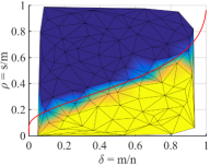
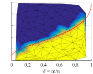
Figure 1: Case 1 Gaussian random matrix: phase-transition diagrams plotted from CV (left), validation (middle), and solution (right) errors where a success recovery is defined by when the respective error quantity is less than $0.1$, using ADMM. Plots using l1  ls, SpaRSA, CGIST, and FPC  AS are very similar to the ADMM results, and thus omitted to avoid repetition.

We now exercise Algorithm 1 to a fixed problem instance that has a sparse solution with $s=25$ nonzero entries. Figure 2 plots the CV, validation, and solution errors versus $m$. Both Figure 2 and a horizontal slice of Figure 1 display the sharp performance change when the critical sample size is crossed, but there are some differences between the two: the former directly plots errors while the latter plots success rates, and the data sets are nested for different $m$ in the former while independently regenerated for each trial in the latter. In Figure 2, the error lines for all solvers share similar behavior, with FPC  AS yielding lower errors compared to others. All solvers display a drastic drop in errors at around 100 sample points, which corresponds to the “cliff” in the phase-transition diagrams—this would be the sample size we want to detect and use for efficient sparse recovery. The change of plot lines from solid (with symbol) to dotted (with no symbol) indicates the stop-sampling point when our algorithm is applied. Overall, they work fairly well and stop sampling in regions around just past the bottom of the sharp drop. Finally, we note that CV errors agree very well with the solution and validation error trends.

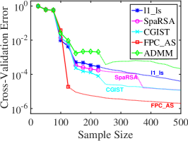
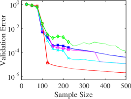
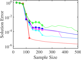
Figure 2: Case 1 Gaussian random matrix: CV (left), validation (middle), and solution (right) errors for fixed problem instance with $n=500$ and $s=25$. Stop-sampling is activated when the plot line turns from solid (with symbols) to dotted (without symbols).

Figure 3 shows the errors from two systems with very sparse (top, $s=1$) and very dense (bottom, $s=400$) solutions, respectively. In both cases, the sharp drop is not immediately noticeable, especially if $\Delta m$ is coarse. For the sparse case, all the errors are already very low even with a very small $m$; for the dense case, the drop occurs only when a large $m$ is achieved (around $500$). Our algorithm is still able to offer reasonable stop-sampling points in both situations. FPC  AS has noticeable spikes in these plots. Additional inspections indicate the spikes are not caused by the grid resolution of $\lambda$, and are likely resulted from within the FPC  AS algorithm.

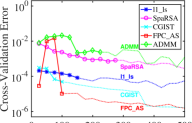
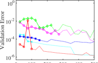
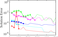
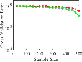
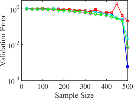
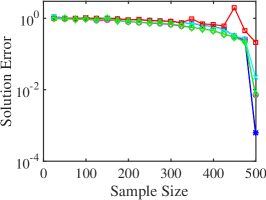
Figure 3: Case 1 Gaussian random matrix: CV (left), validation (middle), and solution (right) errors for fixed problem instance with $n=500$, on a very sparse example $s=1$ (top) and a very dense example $s=400$ (bottom). Stop-sampling is activated when the plot line turns from solid (with symbols) to dotted (without symbols).

Lastly, we present in Figure 4 detailed results of two cases from the fixed problem instance of Figure 2, with an example of good solution using SpaRSA and $m=150$ (top), and an example of bad solution using SpaRSA and $m=25$ (bottom). The training and CV errors at different $\lambda$ are shown in the left column, and the corresponding lowest-CV-error solution stem plots are in the right column. As expected, the training error always decreases as $\lambda$ decreases. For the good solution, the CV error initially decreases as $\lambda$ decreases, and then increases, reflecting overfitting when $\lambda$ becomes too small. The optimal solution is chosen to be at $\lambda^{\ast}$ corresponding to minimal CV error. The stem plot of that solution on the top-right panel shows excellent agreement with the exact solution. For the example of bad solution, the CV error has a plateau of high magnitude in comparison, and the lowest-CV-error solution is in fact at high $\lambda$. The stem plot verifies it to be the zero vector. This outcome implies that when the sample size is too small, CV is still able to reflect and prevent overfitting by reverting to recommend the zero solution (in a sense, a “none” solution is better than the bad solution).

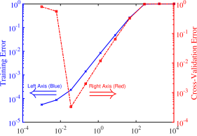
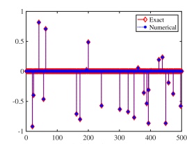
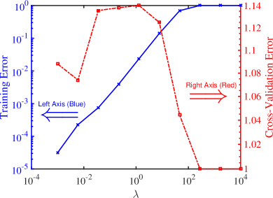
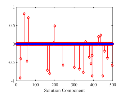
Figure 4: Case 1 Gaussian random matrix: training and CV errors (left; training error in solid blue using left $y$-axis, and CV error in dotted red using right $y$-axis) and corresponding lowest-CV-error solution stem plots (right) for fixed problem instance with $n=500$ and $s=25$ (i.e., encountered in Figure 2), showing an example with good solution (top, using SpaRSA with $m=150$), and an example with bad solution (bottom, using SpaRSA with $m=25$).

4.2 Case 2: random polynomial chaos expansion

We now move on to PCE examples. Consider a Gauss-Hermite PCE of stochastic dimension $n_{s}=5$ and total-order polynomial basis of degree $p=5$, which translates to $n=251$. We use a simple sampling strategy, sampling $\xi_{j}$ corresponding to the PCE germ distribution, i.e., i.i.d. standard normal $\mathcal{N}(0,1)$ for Gauss-Hermite.

Figure 5 shows the phase-transition diagrams using FPC  AS (top) and ADMM (bottom), and plotted based on assessing CV (left), validation (middle), and solution (right) errors. Again, we define a successful reconstruction if the error quantity of interest from a run is less than $0.1$, and the diagram plots the empirical success rate based on $b=10$ repeated trials at each node. The correlation structure of the $A$ matrix induced by the PCE basis leads to a more difficult problem for sparse reconstruction, and the success rates are much lower compared to those in Figure 1. Donoho and Tanner hypothesized that the transition curve from Gaussian random matrix systems exhibits universality properties for many other “well-behaved” distributions as well, particularly with large $n$ [12]. We overlay this theoretical curve in Figure 5, and the empirical transition curves (0.5-probability contours) appear to be much worse in comparison; this phenomenon is also consistent with observations in other papers (e.g., [24, 29]). This PCE-induced distribution of $A$ matrix exhibits a complex correlation structure that likely pushes it outside the “well-behaved” regime, and results in an example that does not comply with the universality hypothesis. Plots using l1  ls, SpaRSA, and CGIST are similar to the ADMM results and thus omitted to avoid repetition, while FPC  AS is observed to produce slightly lower success rates than the other solvers.

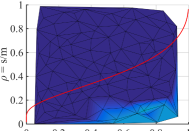
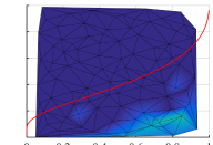
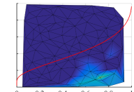
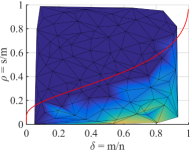
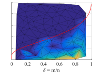
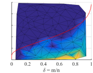
Figure 5: Case 2 random PCE: phase-transition diagrams plotted from CV (left), validation (middle), and solution (right) errors where a success recovery is defined by when the respective error quantity is less than $0.1$, using FPC  AS (top), and ADMM (bottom). Plots using l1  ls, SpaRSA, and CGIST are very similar to the ADMM results, and thus omitted to avoid repetition.

Figure 6 illustrates results for a fixed problem instance where the true solution $x^{\ast}$ is constructed to have $s=20$ randomly selected nonzero elements with values drawn from i.i.d. standard normal $\mathcal{N}(0,1)$. All solvers yield similar error levels, and a sharp drop of error can be observed around $m=100$. FPC  AS is observed to exhibit large error oscillation after $m=100$, which can potentially introduce difficulties for our stop-sampling strategy. However, stop-sampling still does a good job at terminating around the base of the sharp drop. It is interesting to note that while FPC  AS has some undesirable behavior in this case, it yielded the lowest errors in Case 1; the inconsistency in performance may be undesirable overall. The more difficult problem structure can also be observed through the overall higher error values (asymptotes are just below $10^{-1}$) compared to those in the random Gaussian matrix case (achieving $10^{-3}$ or better).

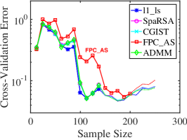
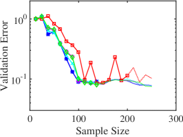
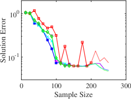
Figure 6: Case 2 random PCE: CV (left), validation (middle), and solution (right) errors for fixed problem instance with $n_{s}=5$, $p=5$ ($n=251$), and $s=20$. Stop-sampling is activated when the plot line turns from solid (with symbols) to dotted (without symbols).

4.3 Case 3: Genz-exponential function

We now explore a more realistic scenario where the solution is not strictly sparse, but compressible (i.e., the sorted coefficient magnitudes decay rapidly), through the Genz-exponential function:

$$y(\xi)=\exp\left({\sum_{j=1}^{n_{s}}a_{j}\xi_{j}}\right).$$ (21)

Let the stochastic dimension be $n_{s}=5$, and the exponential coefficients endowed with a power rule decay of $a_{j}=j^{-1}$. Gauss-Hermite PCEs of different polynomial orders are constructed to approximate Equation 21 via evaluations at $\xi_{j}$ samples drawn from i.i.d. standard normal $\mathcal{N}(0,1)$. This problem is challenging on several fronts. First, there is truncation error for any finite-order polynomial approximation to the exponential form of Equation 21—i.e., modeling error is always present. Second, the best polynomial approximation is not expected to be strictly sparse as a result of both truncation and that $a_{j}$ is not sparse even though it is decaying. However, it may be near-sparse, and it would still be valuable to find a solution that balances approximation error and sparsity.

We compare PCEs of total-order $p=3$, $5$, and $7$ in representing Equation 21. Intuitively, one expects higher order polynomials to offer richer basis sets and thus smaller modeling error (i.e., lower achievable error). However, larger basis sets also mean larger $n$, and produce systems that could be harder to solve, both in terms of computational cost and numerical accuracy (i.e., higher numerical error). Let us elaborate on these two points. Imagine we are comparing two total-order polynomial basis sets with degrees $p_{1}$ and $p_{2}$ (assume $p_{1}<p_{2}$) under a fixed data set (and thus also the same sample size $m$). If the true data-generating model were less than $p_{1}$ degree polynomial, then neither choice has modeling error. The richer basis set form $p_{2}$ has no modeling benefit while the undersampling ratio $\delta=m/n$ (recall $n$ is the number of columns of $A$) would be lower, which generally translates to a lower probability of successful recovery if everything else remains the same (c.f. phase-transition diagrams in Figures 1 and 5). In the case where there is modeling error, the coefficient of the new terms from $p_{2}$ may or may not have non-negligible magnitudes, and so the overall sparsity ratio $\rho=s/m$ (recall $s$ is the number of non-zero elements) can change in either direction. Since the polynomial spectrum of an exponential form Equation 21 generally decays with order, we expect $\rho$ to not decrease for this case. Overall, the effects of achievable error and numerical error are unclear when polynomial order is increased, and certainly are problem dependent.

Figure 7 illustrates the CV (left) and validation errors (right) for $p=3$ (top), $p=5$ (middle), and $p=7$ (bottom), which correspond to $n=55$, $251$, and $791$, respectively. To ensure a fair comparison, a common $m$ range is used, up to $m=790$, which corresponds to just before when $p=7$ systems are no longer underdetermined. Even though ordinary least squares (OLS) becomes a possible option for overdetermined regions of $p=3$ and $5$, we provide results using the same CS solvers for a consistent assessment. Separate OLS results are also plotted with solid black lines, and we can see they are generally very close to results from the CS solvers. This is not surprising, since as $m$ increases, the contribution from the $\ell_{2}$-norm term increases while the $\ell_{1}$-norm term remains fixed, and so the uLASSO Equation 4 tends toward OLS (although the OLS solution is much cheaper to obtain). From the new plots, the error levels are visibly better when moving from $p=3$ to $5$, but only improves marginally (in fact, slightly worse in certain regions) when switching to $p=7$. This implies improvement to modeling error dominates up to $p=5$, but the increased complexity starts to outweigh this benefit at $p=7$.

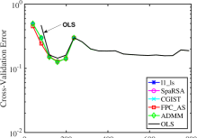
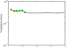
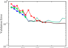
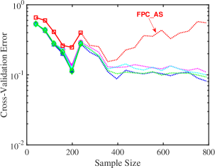
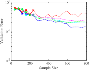
Figure 7: Case 3 Genz-exponential function: CV (left) and validation (right) errors for fixed problem instance with $n_{s}=5$, using $p=3$ ($n=55$) (top), $p=5$ ($n=251$) (middle), and $p=7$ ($n=791$) (bottom). Stop-sampling is activated when the plot line turns from solid (with symbols) to dotted (without symbols). OLS results are also included for when $p=3$ and $p=5$ systems become overdetermined ($m>55$ and $m>251$, respectively), and are shown as solid black lines without symbols.

Figure 8 shows results for Equation 21 with $a_{2}=a_{3}=0$ while all other coefficients remain $a_{j}=j^{-1}$ as before, which induces a more compressible solution. Compared to the compressible (decaying coefficients) version in Figure 7, the new system has similar trends but with sharper error decreases that also occur at smaller $m$ values, and the error levels are overall lower. Solution stem plots from $p=5$ using OLS with $m=790$ are shown in Figure 9 for both the compressible and sparse versions; solutions from CV solvers are similar and omitted. All these observations match our intuitive expectations, where a sparser problem would be easier to solve. Furthermore, the difference in performance is small between the two versions, indicating that the numerical methods would still work well even when zero-coefficients are contaminated.

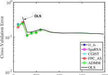
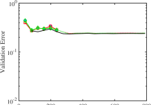
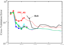
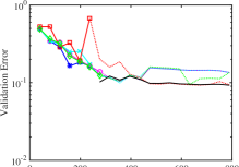
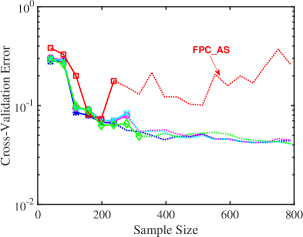
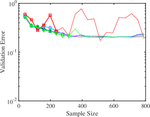
Figure 8: Case 3 Genz-exponential function with artificially imposed sparsity by setting $a_{2}=a_{3}=0$ in Equation 21: CV (left) and validation (right) errors for fixed problem instance with $n_{s}=5$, using $p=3$ ($n=55$) (top), $p=5$ ($n=251$) (middle), and $p=7$ ($n=791$) (bottom). Stop-sampling is activated when the plot line turns from solid (with symbols) to dotted (without symbols). OLS results are also included for when $p=3$ and $p=5$ systems become overdetermined ($m>55$ and $m>251$, respectively), and are shown as solid black lines without symbols.

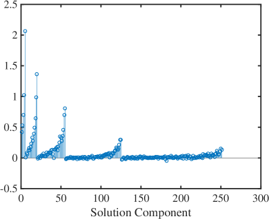
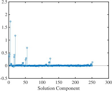
Figure 9: Case 3 Genz-exponential function: solution stem plot for $n_{s}=5$, $p=5$ ($n=251$), using OLS with $m=790$ (Figure 7 middle row right-most end of the black line) (left), and its sparse version counterpart (Figure 8 middle row right-most end of the black line) (right).

All solvers yield similar error levels for this case, with the exception of FPC  AS, which produces higher error levels that can also be quite oscillatory especially at higher polynomial orders. The stop-sampling heuristic performs well in detecting the lower end regions of the largest error drops.

4.4 Case 4: Jet-in-Crossflow (JXF) application

We now describe a study involving simulations of the physical phenomenon when a jet interacts in a crossflow. JXF is frequently encountered in many different engineering applications, such as fuel injection and combustor cooling in gas turbine engines and plume dispertion. A comprehensive review can be found in Mahesh [35]. In this paper we focus on a setup that corresponds to the HiFiRE program [25]. This configuration is relevant for the design of supersonic combusting ramjet (scramjet) engines [27]. Having a fundamental understanding of this physical behavior is thus extremely valuable for producing accurate simulations and high-performing designs.

As an initial exploratory step of the overall design project, this setup involves simulations of supersonic turbulent fuel jet and crossflow in a simplified two-dimensional computational domain presented in Figure 10. While 2D turbulence phenomenon is not physically realistic, it is useful in providing physical insights and for testing our CS methodology. The crossflow travels from left to right in the $x$-direction (streamwise), and remains supersonic throughout the entire domain. The geometry is symmetric about the top in the $y$-direction (wall-normal), and is endowed with symmetry boundary conditions. Normalized spatial distance units $x/d$ and $y/d$ are used in subsequent descriptions and results, where $d=3.175$ mm is the diameter of the fuel injector. The bottom of the geometry is a solid wall, with a downward slope of $1.3^{\circ}$ starting from $x_{\textnormal{kink}}/d=3.94$. Fuel is introduced at $x_{\textnormal{inj}}/d=16.75$ through an injector aligned an angle of $15^{\circ}$ from the wall. The fuel is the JP-7 surrogate, which consists of 36% methane and 64% ethylene. Combustion is turned off for this study, allowing a targeted investigation of the interaction between the fuel jet and the supersonic crossflow without the effects of chemical heat release.

Figure 10: Case 4 JXF application: computational schematic of the injected fuel jet in a supersonic crossflow. All distance quantities shown are normalized by the injector diameter $d=3.175$ mm. For example, $x_{\textnormal{qoi}}=40\,d=12.7$ cm.

Large eddy simulation (LES) calculations are then carried out using the RAPTOR code framework developed by Oefelein [39, 38]. The code performs compressible numerical simulation and has been optimized to meet the strict algorithmic requirements imposed by the LES formalism. Specifically, it solves the fully-coupled conservation equations of mass, momentum, and total-energy, under high Reynolds number, high Mach number, and with real-gas and liquid phases. It also accounts for detailed thermodynamics and transport processes at the molecular level. A relatively coarse grid is used, where each grid has size $d/8$. Each simulation requires around 12 total CPU-hours to produce statistically converged results.

We let $n_{s}=24$ model parameters be uncertain with distributions described in Table 2. The wall temperature ($T_{w}$) boundary condition is a function of $x/d$, and hence is a random field (RF). $T_{w}$ is thus represented using the Karhunen-Loève expansion (KLE) (e.g., [20]), which is built employing the eigenstructure of the covariance function of the RF to achieve an optimal representation. We employ a Gaussian RF with a square exponential covariance structure along with a correlation length that is similar to the largest turbulent eddies (i.e., the size of the crossflow inlet). The mean temperature profile is constructed by averaging temperature profile results from a small set of separate adiabatic simulations. The correlation length employed leads to a rapid decay in characteristic-mode amplitudes, allowing us to capture about 90% of the total variance of this RF with only a ten-dimensional KLE. The wall temperature is further assumed to be constant in time. All other parameters are endowed with uniform distributions. More details on the KLE model are presented in Huan et al. [27]. The mixture of Gaussian and uniform distributions is accommodated by a hybrid Gauss-Hermite and Legendre-Uniform PCE, with the appropriate type used for each dimension. The model output quantity of interest (QoI) is selected to be the time-averaged stagnation pressure $P_{\textnormal{stag}}$ located at $x_{\textnormal{qoi}}/d=100$ (near the outlet) and spatially averaged over $y/d$. $P_{\textnormal{stag}}$ is an important output in engine design, since the stagnation pressure differential between inlet and outlet is a relevant component in computing the thrust. Examples of $P_{\textnormal{stag}}$ plotted over $y/d$, i.e. before spatial-averaging, are shown in Figure 11; the wall boundary effect of reducing the $P_{\textnormal{stag}}$ (left side of the plot) is evident.

Table 2: Case 4 JXF application: uncertain model input parameters. The uncertain distributions are uniform across the ranges shown, with the exception for the bottom wall temperature which is expressed as a KLE involving 10 standard Gaussian random variables.

Parameter	Range	Description
Inlet boundary conditions
$p_{0}$	$[1.406,1.554]\times 10^{6}$ Pa	Stagnation pressure
$T_{0}$	$[1472.5,1627.5]$ K	Stagnation temperature
$M_{0}$	$[2.259,2.761]$	Mach number
$\delta_{i}$	$[2,6]\times 10^{-3}$ m	Boundary layer thickness
$I_{i}$	$[0,0.05]$	Turbulence intensity magnitude
$L_{i}$	$[0,8]\times 10^{-3}$ m	Turbulence length scale
Fuel inflow boundary conditions
$\dot{m}_{f}$	$[6.633,8.107]\times 10^{-3}$ kg/s	Mass flux
$T_{f}$	$[285,315]$ K	Static temperature
$M_{f}$	$[0.95,1.05]$	Mach number
$I_{f}$	$[0,0.05]$	Turbulence intensity magnitude
$L_{f}$	$[0,1]\times 10^{-3}$ m	Turbulence length scale
Turbulence model parameters
$C_{R}$	$[0.01,0.06]$	Modified Smagorinsky constant
$Pr_{t}$	$[0.5,1.7]$	Turbulent Prandtl number
$Sc_{t}$	$[0.5,1.7]$	Turbulent Schmidt number
Wall boundary conditions
$T_{w}$	Expansion in 10 params	Wall temperature represented via
	of i.i.d. $\mathcal{N}(0,1)$	Karhunen-Loève expansion (KLE)

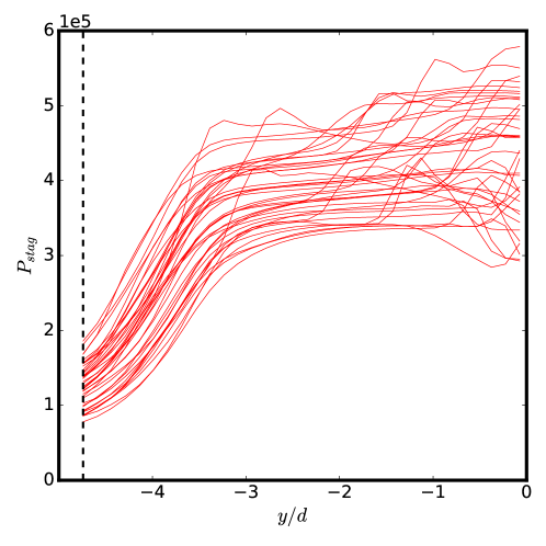
Figure 11: Case 4 JXF application: profiles of time-averaged (normalized) $P_{\textnormal{stag}}$ plotted over $y/d$, at fixed $x_{\textnormal{qoi}}/d=100$, for selected runs of different parameter settings. Each red line is the profile of an independent simulation drawn from the 24-dimensional parameter space according to the distributions described in Table 2. The vertical dotted line on the left side is the bottom wall.

PCEs with total-order polynomial degrees $p=2$ ($n=324$) and $p=3$ ($n=2924$) are constructed using Algorithm 1, and their CV errors are shown in Figure 12. The left and right plots correspond to results from $p=2$ and $3$ for $m$ sizes up to 1822, and the inset on the left panel shows results using a finer $m$ discretization up to $m=324$, which corresponds to just before when $p=2$ systems are no longer underdetermined. OLS results are also included when $p=2$ systems become overdetermined, and the difference between CS and OLS results decreases as $m$ increases, as expected. The error levels are slightly lower for $p=3$ than $2$, implying that the overall advantage from the enriched $p=3$ basis is present, but not significant. (Additional testing using $p=4$, not shown in this paper, also produced similar solutions, thus supporting that $p=3$ is appropriate for this application.) The trends appear smooth and well-behaved, with a rather rapid drop at around $m=100$ for $p=2$ ($n=324$), and $m=300$ for $p=3$ ($n=2924$), hinting at a sparse or compressible solution. Stop-sampling is able to capture the drop well for the $p=3$ case ($p=2$ errors do not drop sufficiently). All solvers perform similarly for $p=2$ but move apart for $p=3$ especially at low $m$, with ADMM and FPC  AS yielding higher errors than others. FPC  AS also experiences large error oscillations.

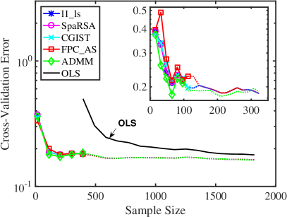
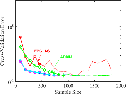
Figure 12: Case 4 JXF application: CV error for $n_{s}=24$, using $p=2$ ($n=324$) (left) and $p=3$ ($n=2924$) (right). The inset on the left panel shows results using a finer $m$ discretization up to $m=323$, which corresponds to just before when $p=2$ systems become underdetermined. Stop-sampling is activated when the plot line turns from solid (with symbols) to dotted (without symbols). OLS results are also included for when $p=2$ systems become overdetermined ($m>324$), and are shown as solid black lines without symbols.

Since the true solution is unknown, we study the best numerical solution encountered in our computations, which is produced by $p=3$ using SpaRSA with $m=1822$ (Figure 12 right panel, right-most end of the magenta line). The training and CV errors as a function of $\lambda$ are shown in the left panel in Figure 13, and the solution stem plot for the lowest-CV-error solution is shown on the right. The solution indeed appears sparse, confirming our earlier hypothesis. The most dominating coefficients, in decreasing magnitude, correspond to the linear terms in $M_{0}$, $p_{0}$, $\delta_{i}$, and $L_{i}$. This is consistent with the global sensitivity analysis performed in [27], where the leading total sensitivity Sobol indices for $P_{\textnormal{stag}}$ were $\{M_{0}:0.904\}$, $\{p_{0}:0.033\}$, $\{\delta_{i}:0.032\}$, and $\{L_{i}:0.031\}$. While the Sobol indices are not exactly equal to the linear coefficients (Sobol indices also include sum of coefficients-squared from higher order orthnormal basis terms), they are dominated by the linear coefficients in this case. This also explains the rather small improvement of $p=3$ compared to $p=2$ results in Figure 12, as most of the third-order terms have negligible coefficients. These observations are consistent with physics-based intuition: since the current setup does not involve combustion, one would expect the crossflow conditions to dictate the impact on the QoI behavior.

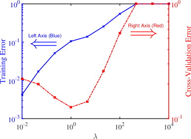
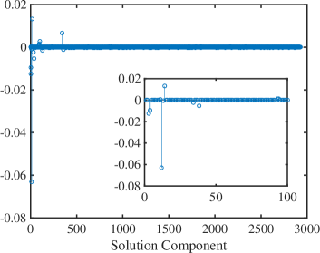
Figure 13: Case 4 JXF application: training and CV errors (left; training error in solid blue using left $y$-axis, and CV error in dotted red using right $y$-axis) and corresponding lowest-CV-error solution stem plot (right) for $n_{s}=24$, $p=3$ ($n=2924$), using SpaRSA with $m=1822$ (Figure 12 right panel right-most end of the magenta line). The inset on the right panel shows the stem plot zoomed in for the first 100 components. This is the best solution obtained for case 4, and serves as a reference for subsequent comparisons.

In contrast to Figure 13, an example of a bad solution is shown in Figure 14, produced by $p=3$ using FPC  AS with $m=364$ (Figure 12 right panel fourth point of red line). Similar to the example in Figure 4, the CV error has a “bump” instead of a “dip”. In this case, the lowest-CV-error solution is at the smallest $\lambda$ in the range investigated. The solution stem plot is shown on the right panel, and the small $\lambda$ induces a dense vector with many non-zero components clearly visible. The highest magnitude coefficients, however, are still correctly identified.

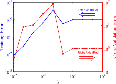
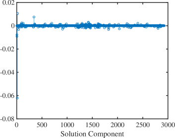
Figure 14: Case 4 JXF application: training and CV errors (left; training error in solid blue using left $y$-axis, and CV error in dotted red using right $y$-axis) and corresponding lowest-CV-error solution stem plot (right) for $n_{s}=24$, $p=3$ ($n=2924$), using FPC  AS with $m=364$ (Figure 12 right panel fourth point of red line). This is an example of bad solution compared to the reference in Figure 13.

4.5 Timing discussions

All computations in Algorithm 1 are performed on a 1400 MHz AMD processor with a very small memory requirement, and the average CPU times per system solve (including corresponding CV solves) are summarized in Figure 15. Overall, FPC  AS and ADMM produce CPU times that are lower in the group, l1  ls and CGIST have less consistent performance and can be very fast in some situations while slow in others, and SpaRSA is usually in the middle. Since FPC  AS is sometimes observed to have slightly higher and oscillatory error levels in our test cases, we find ADMM to be a good practical solver to start with.

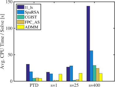
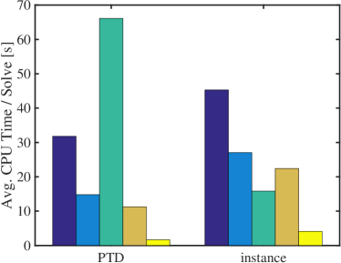
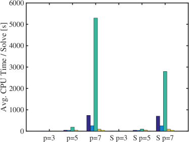
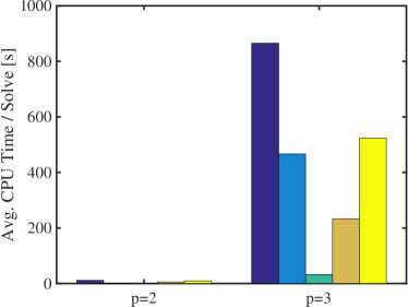
Figure 15: Average CPU time of Algorithm 1 per system solve for case 1 (top left), case 2 (top right), case 3 (bottom left), case 4 (bottom right), and their subcases (each group across the horizontal axis). “PTD” refers to phase-transition diagram computations, “instance” refers to the main fixed problem instance, and “S p=3” corresponds to the Genz-exponential case with artificially imposed sparsity.

Figure 16 further illustrates the CPU time trend across $\lambda$ for case 2’s fixed problem instance (similar trends are observed in other cases). Each red line represents the system solve (including CV) at a different $m$. Although not labeled in the figure, the more computationally expensive plot lines generally correspond to larger $m$ values. The computational costs increase with smaller $\lambda$ for all solvers, and with the exception for ADMM they also decrease with larger $\lambda$ (and the solution tending towards the zero vector). ADMM has an interesting “dip” shape, is overall computationally less expensive in this case, but can become the more expensive choice when $\lambda$ is large enough. A solver other than ADMM thus may be advisable for large values of $\lambda$.

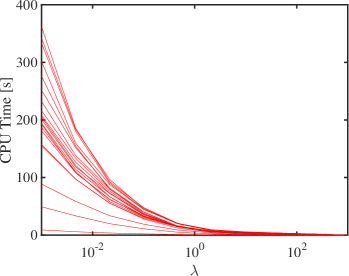
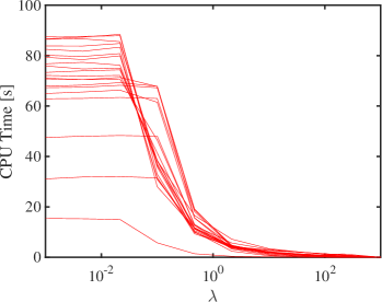
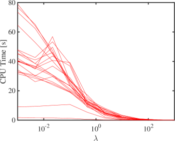
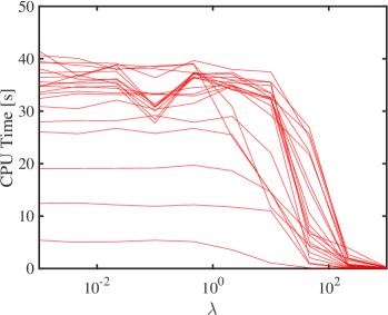
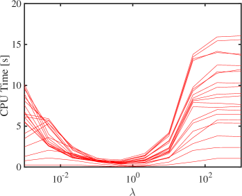
Figure 16: CPU time as a function of $\lambda$ for case 2 random PCE, fixed problem instance with $n_{s}=5$, $p=5$ ($n=251$), and $s=20$, using solver l1  ls and SpaRSA (top left and right), CGIST and FPC  AS (middle left and right), and ADMM (bottom). Each red line corresponds to a system solve (including CV) at a different $m$.

5 Conclusions

In this paper, we performed numerical investigations employing several CS solvers that target the unconstrained LASSO formulation, with a focus on linear systems that rise in PCE constructions. With core solvers of l1  ls, SpaRSA, CGIST, FPC  AS, and ADMM, we implemented techniques to mitigate overfitting through an automated selection of regularization constant $\lambda$ based on minimizing the $K$-fold CV error, and a heuristic strategy to guide the stop-sampling decision using trends on CV error decay. Practical recommendations on parameter settings for these techniques were provided and discussed.

The overall method is then applied to a series of numerical examples of increasing complexity: Gaussian random matrix, random PCE, PCE approximations to a Genz-exponential model, and large eddy simulations of supersonic turbulent jet-in-crossflow involving a 24-dimensional input. We produced phase-transition diagrams for the Gaussian random matrix test that matched well with theoretical results, and also for the random PCE example that experienced more difficult recovery. The latter involved a complex correlation structure in the linear system matrices induced by PCE, resulting in an example that does not comply with the phase-transition universality hypothesis. PCEs of different degrees were explored for the Genz-exponential study, illustrating the effects of modeling error and tradeoff between accuracy and computational costs. The jet-in-crossflow case produced results that are consistent with physical intuition and previous global sensitivity analysis investigation. Furthermore, it demonstrated the practicability of conducting CS for a realistic, high-dimensional physical application. Overall, the accuracy and computational performance for all CS solvers were similar, with ADMM showing some advantages with consistent low errors and computational times for several of the test cases studied in this paper.

Interesting future directions of research include comparisons with BCS methods, the incorporation of front-tracking (adaptive basis enrichment) informed by CV error, and investigations on the effects of overfitting when multiple models of different fidelity are available.

Appendix A Default Parameters for CS Solvers

Tables 3, 4, 5, 6 and 7 show the default parameters for CS solvers adopted in this study.

Table 3: Default parameters for l1  ls.

Parameter	Value
tar_gap	$10^{3}$
eta	$10^{3}$
pcgmaxi	$5000$

Table 4: Default parameters for SpaRSA.

Parameter	Value	Parameter	Value	Parameter	Value
StopCriterion	$2$	Initialization	$0$	Eta	$2$
ToleranceA	$10^{-2}$	BB_variant	$1$	Continuation	$0$
Debias	$0$	BB_cycle	$1$	AlphaMin	$10^{-30}$
MaxiterA	$1000$	Monotone	$0$	AlphaMax	$10^{30}$
MiniterA	$5$	Safeguard	$0$

Table 5: Default parameters for CGIST.

Parameter	Value
guess	$0$
continuation_if_needed	true
tol	$10^{-4}$
max_iter	$25000$

Table 6: Default parameters for FPC  AS. To enable the solver for overdetermined systems, replace all “$m$” terms by “$\min(m,n)$”.

Parameter	Value	Parameter	Value	Parameter	Value
x0	$0$	tau_min	$10^{-4}$	eta	$0.1$
init	$2$	tau_max	$10^{3}$	sub_mxitr	$50$
tol_eig	$10^{-4}$	mxitr	$1000$	lbfgs_m	$5$
scale_A	$0$	gtol	$10^{-6}$	ls_meth	Hybridls
eps	$10^{-16}$	gtol_scale_x	$10^{-12}$	sub_opt_meth	pcg
zero	$10^{-10}$	f_rel_tol	$10^{-20}$	kappa_g_d	$10$
dynamic_zero	$1$	f_value_tol	$0$	kappa_rho	$10$
minK	$\lfloor m/2\rfloor$	ls_mxitr	$5$	tol_start_sub	$10^{-6}$
maxK	$m$	gamma	$0.85$	min_itr_shrink	$3$
hard_truncate	$1$	c	$10^{-3}$	max_itr_shrink	$20$
tauD	$\begin{aligned} &\min(1.999,\\ &-1.665\frac{m}{n}+2.665)\end{aligned}$	beta	$0.5$

Table 7: Default parameters for ADMM.

Parameter	Value
rho	$1.0$
alpha	$1.0$

References

- [1] H. Akaike, A New Look at the Statistical Model Identification, IEEE Transactions on Automatic Control, 19 (1974), pp. 716–723, https://doi.org/10.1109/TAC.1974.1100705.
- [2] S. Babacan, R. Molina, and A. Katsaggelos, Bayesian Compressive Sensing Using Laplace Priors, IEEE Transactions on Image Processing, 19 (2010), pp. 53–63, https://doi.org/10.1109/TIP.2009.2032894.
- [3] V. Barthelmann, E. Novak, and K. Ritter, High dimensional polynomial interpolation on sparse grids, Advances in Computational Mathematics, 12 (2000), pp. 273–288, https://doi.org/10.1023/A:1018977404843.
- [4] G. Blatman and B. Sudret, Adaptive sparse polynomial chaos expansion based on least angle regression, Journal of Computational Physics, 230 (2011), pp. 2345–2367, https://doi.org/10.1016/j.jcp.2010.12.021.
- [5] S. Boyd, N. Parikh, E. Chu, B. Peleato, and J. Eckstein, Distributed Optimization and Statistical Learning via the Alternating Direction Method of Multipliers, Foundations and Trends in Machine Learning, 3 (2010), pp. 1–122, https://doi.org/10.1561/2200000016.
- [6] S. Boyd, N. Parikh, E. Chu, B. Peleato, and J. Eckstein, Solve LASSO via ADMM, 2011, https://web.stanford.edu/~boyd/papers/admm/lasso/lasso.html (accessed 2017-07-02).
- [7] E. J. Candès, J. Romberg, and T. Tao, Robust Uncertainty Principles: Exact Signal Reconstruction From Highly Incomplete Frequency Information, IEEE Transactions on Information Theory, 52 (2006), pp. 489–509, https://doi.org/10.1109/TIT.2005.862083.
- [8] S. S. Chen, D. L. Donoho, and M. A. Saunders, Atomic Decomposition by Basis Pursuit, SIAM Review, 43 (2001), pp. 129–159, https://doi.org/10.1137/S003614450037906X.
- [9] G. Davis, S. Mallat, and M. Avellaneda, Adaptive greedy approximations, Constructive Approximation, 13 (1997), pp. 57–98, https://doi.org/10.1007/BF02678430.
- [10] D. L. Donoho, Compressed sensing, IEEE Transactions on Information Theory, 52 (2006), pp. 1289–1306, https://doi.org/10.1109/Tit.2006.871582.
- [11] D. L. Donoho, For Most Large Underdetermined Systems of Linear Equations the Minimal -norm Solution Is Also the Sparsest Solution, Communications on Pure and Applied Mathematics, 59 (2006), pp. 797–829, https://doi.org/10.1002/cpa.20132.
- [12] D. L. Donoho and J. Tanner, Observed universality of phase transitions in high-dimensional geometry, with implications for modern data analysis and signal processing, Philosophical Transactions of the Royal Society A: Mathematical, Physical and Engineering Sciences, 367 (2009), pp. 4273–4293, https://doi.org/10.1098/rsta.2009.0152.
- [13] D. L. Donoho and J. Tanner, Precise Undersampling Theorems, Proceedings of the IEEE, 98 (2010), pp. 913–924, https://doi.org/10.1109/JPROC.2010.2045630.
- [14] B. Efron, T. Hastie, I. Johnstone, and R. Tibshirani, Least angle regression, The Annals of Statistics, 32 (2004), pp. 407–499, https://doi.org/10.1214/009053604000000067.
- [15] M. S. Eldred, L. W. T. Ng, M. F. Barone, and S. P. Domino, Multifidelity Uncertainty Quantification Using Spectral Stochastic Discrepancy Models, in Handbook of Uncertainty Quantification, Springer International Publishing, Cham, 2015, pp. 1–45, https://doi.org/10.1007/978-3-319-11259-6_25-1.
- [16] O. G. Ernst, A. Mugler, H.-J. Starkloff, and E. Ullmann, On the convergence of generalized polynomial chaos expansions, ESAIM: Mathematical Modelling and Numerical Analysis, 46 (2012), pp. 317–339, https://doi.org/10.1051/m2an/2011045.
- [17] N. Fajraoui, S. Marelli, and B. Sudret, On optimal experimental designs for sparse polynomial chaos expansions, 2017, https://arxiv.org/abs/1703.05312.
- [18] T. Gerstner and M. Griebel, Numerical integration using sparse grids, Numerical Algorithms, 18 (1998), pp. 209–232, https://doi.org/10.1023/A:1019129717644.
- [19] T. Gerstner and M. Griebel, Dimension-Adaptive Tensor-Product Quadrature, Computing, 71 (2003), pp. 65–87, https://doi.org/10.1007/s00607-003-0015-5.
- [20] R. G. Ghanem and P. D. Spanos, Stochastic Finite Elements: A Spectral Approach, Springer New York, New York, NY, 1st ed., 1991.
- [21] T. Goldstein and S. Setzer, High-order methods for basis pursuit, Tech. Report CAM Report 10-41, University of California Los Angeles, 2010.
- [22] T. Goldstein and S. Setzer, CGIST: A Fast and Exact Solver for L1 Minimization, 2011, http://tag7.web.rice.edu/CGIST.html (accessed 2017-07-02).
- [23] J. H. Halton, On the efficiency of certain quasi-random sequences of points in evaluating multi-dimensional integrals, Numerische Mathematik, 2 (1960), pp. 84–90, https://doi.org/10.1007/BF01386213.
- [24] J. Hampton and A. Doostan, Compressive sampling of polynomial chaos expansions: Convergence analysis and sampling strategies, Journal of Computational Physics, 280 (2015), pp. 363–386, https://doi.org/10.1016/j.jcp.2014.09.019.
- [25] N. E. Hass, K. F. Cabell, and A. M. Storch, HIFiRE Direct-Connect Rig (HDCR) Phase I Ground Test Results from the NASA Langley Arc-Heated Scramjet Test Facility, Tech. Report CR-2010-002215, NASA, 2010.
- [26] T. Hastie, R. Tibshirani, and J. Friedman, The Elements of Statistical Learning, Springer, New York, NY, 2nd ed., 2009.
- [27] X. Huan, C. Safta, K. Sargsyan, G. Geraci, M. S. Eldred, Z. P. Vane, G. Lacaze, J. C. Oefelein, and H. N. Najm, Global Sensitivity Analysis and Estimation of Model Error, Toward Uncertainty Quantification in Scramjet Computations, AIAA Journal, 56 (2018), pp. 1170–1184, https://doi.org/10.2514/1.J056278.
- [28] J. D. Jakeman, M. S. Eldred, and K. Sargsyan, Enhancing -minimization estimates of polynomial chaos expansions using basis selection, Journal of Computational Physics, 289 (2015), pp. 18–34, https://doi.org/10.1016/j.jcp.2015.02.025.
- [29] J. D. Jakeman, A. Narayan, and T. Zhou, A Generalized Sampling and Preconditioning Scheme for Sparse Approximation of Polynomial Chaos Expansions, SIAM Journal on Scientific Computing, 39 (2017), pp. A1114–A1144, https://doi.org/10.1137/16M1063885.
- [30] S. Ji, Y. Xue, and L. Carin, Bayesian compressive sensing, IEEE Transactions on Signal Processing, 56 (2008), pp. 2346–2356, https://doi.org/10.1109/TSP.2007.914345.
- [31] R. E. Kass and A. E. Raftery, Bayes Factor, Journal of American Statistical Association, 90 (1995), pp. 773–795, https://doi.org/10.2307/2291091.
- [32] S.-J. Kim, K. Koh, M. Lustig, S. Boyd, and D. Gorinevsky, An Interior Point Method for Large-Scale -Regularized Least Squares, IEEE Journal of Selected Topics in Signal Processing, 1 (2007), pp. 606–617, https://doi.org/10.1109/JSTSP.2007.910971.
- [33] K. Koh, S.-J. Kim, and S. Boyd, Simple Matlab Solver for l1-regularized Least Squares Problems, beta version, 2008, https://stanford.edu/~boyd/l1_ls/ (accessed 2017-07-02).
- [34] O. P. Le Maître and O. M. Knio, Spectral Methods for Uncertainty Quantification: with Applications to Computational Fluid Dynamics, Springer Netherlands, Houten, Netherlands, 2010.
- [35] K. Mahesh, The Interaction of Jets with Crossflow, Annual Review of Fluid Mechanics, 45 (2013), pp. 379–407, https://doi.org/10.1146/annurev-fluid-120710-101115.
- [36] D. M. Malioutov, S. R. Sanghavi, and A. S. Willsky, Sequential Compressed Sensing, IEEE Journal of Selected Topics in Signal Processing, 4 (2010), pp. 435–444, https://doi.org/10.1109/JSTSP.2009.2038211.
- [37] H. N. Najm, Uncertainty Quantification and Polynomial Chaos Techniques in Computational Fluid Dynamics, Annual Review of Fluid Mechanics, 41 (2009), pp. 35–52, https://doi.org/10.1146/annurev.fluid.010908.165248.
- [38] J. C. Oefelein, Simulation and Analysis of Turbulent Multiphase Combustion Processes at High Pressures, PhD thesis, The Pennsylvania State University, 1997.
- [39] J. C. Oefelein, Large eddy simulation of turbulent combustion processes in propulsion and power systems, Progress in Aerospace Sciences, 42 (2006), pp. 2–37, https://doi.org/10.1016/j.paerosci.2006.02.001.
- [40] J. Peng, J. Hampton, and A. Doostan, A weighted -minimization approach for sparse polynomial chaos expansions, Journal of Computational Physics, 267 (2014), pp. 92–111, https://doi.org/10.1016/j.jcp.2014.02.024.
- [41] H. Rauhut and R. Ward, Sparse Legendre expansions via -minimization, Journal of Approximation Theory, 164 (2012), pp. 517–533, https://doi.org/10.1016/j.jat.2012.01.008.
- [42] K. Sargsyan, C. Safta, H. N. Najm, B. J. Debusschere, D. Ricciuto, and P. Thornton, Dimensionality Reduction for Complex Models Via Bayesian Compressive Sensing, International Journal for Uncertainty Quantification, 4 (2014), pp. 63–93, https://doi.org/10.1615/Int.J.UncertaintyQuantification.2013006821.
- [43] G. Schwarz, Estimating the Dimension of a Model, The Annals of Statistics, 6 (1978), pp. 461–464, https://doi.org/10.1214/aos/1176344136.
- [44] J. Tanner, Phase Transitions of the Regular Polytopes and Cone, 2012, https://people.maths.ox.ac.uk/tanner/polytopes.shtml (accessed 2017-07-03).
- [45] E. van den Berg and M. P. Friedlander, Probing the Pareto Frontier for Basis Pursuit Solutions, SIAM Journal on Scientific Computing, 31 (2009), pp. 890–912, https://doi.org/10.1137/080714488.
- [46] L. Wasserman, Bayesian Model Selection and Model Averaging, Journal of Mathematical Psychology, 44 (2000), pp. 92–107, https://doi.org/10.1006/jmps.1999.1278.
- [47] Z. Wen, W. Yin, D. Goldfarb, and Y. Zhang, A Fast Algorithm for Sparse Reconstruction Based on Shrinkage, Subspace Optimization, and Continuation, SIAM Journal on Scientific Computing, 32 (2010), pp. 1832–1857, https://doi.org/10.1137/090747695.
- [48] S. J. Wright, R. D. Nowak, and M. A. T. Figueiredo, SpaRSA: Sparse Reconstruction by Separable Approximation, version 2.0, 2009, http://www.lx.it.pt/~mtf/SpaRSA/ (accessed 2017-07-02).
- [49] S. J. Wright, R. D. Nowak, and M. A. T. Figueiredo, Sparse Reconstruction by Separable Approximation, IEEE Transactions on Signal Processing, 57 (2009), pp. 2479–2493, https://doi.org/10.1109/TSP.2009.2016892.
- [50] D. Xiu, Fast Numerical Methods for Stochastic Computations: A Review, Communications in Computational Physics, 5 (2009), pp. 242–272.
- [51] D. Xiu and G. E. Karniadakis, The Wiener-Askey Polynomial Chaos for Stochastic Differential Equations, SIAM Journal on Scientific Computing, 24 (2002), pp. 619–644, https://doi.org/10.1137/S1064827501387826.
- [52] W. Yin and Z. Wen, FPC_AS: A MATLAB Solver for L1-Regularization Problems, version 1.21, 2010, http://www.caam.rice.edu/~optimization/L1/FPC_AS/ (accessed 2017-07-02).