Ricci-Gauss-Bonnet holographic dark energy

Abstract

We present a model of holographic dark energy in which the Infrared cutoff is determined by both the Ricci and the Gauss-Bonnet invariants. Such a construction has the significant advantage that the Infrared cutoff, and consequently the holographic dark energy density, does not depend on the future or the past evolution of the universe, but only on its current features, and moreover it is determined by invariants, whose role is fundamental in gravitational theories. We extract analytical solutions for the behavior of the dark energy density and equation-of-state parameters as functions of the redshift. These reveal the usual thermal history of the universe, with the sequence of radiation, matter and dark energy epochs, resulting in the future to a complete dark energy domination. The corresponding dark energy equation-of-state parameter can lie in the quintessence or phantom regime, or experience the phantom-divide crossing during the cosmological evolution, and its asymptotic value can be quintessence-like, phantom-like, or be exactly equal to the cosmological-constant value. Finally, we extract the constraints on the model parameters that arise from Big Bang Nucleosynthesis.

I Introduction

According to the concordance paradigm of cosmology the universe, after being in a long matter-dominated epoch, has entered in an accelerating phase. Although the reasonable explanation is that the cause of this acceleration is the cosmological constant Peebles:2002gy , the possibility of a dynamical nature, as well as the need to additionally describe the early-time acceleration era (inflation) too, led to the need of introducing extra degree(s) of freedom beyond the standard framework of general relativity and Standard Model of particles. One can attribute these extra degrees of freedom to new, exotic forms of matter, such as in the dark energy concept (for reviews see Copeland:2006wr ; Cai:2009zp ), or alternatively, one can consider the extra degrees of freedom to have gravitational origin, i.e. to arise from a gravitational modification that possesses general relativity as a particular limit (see Nojiri:2006ri ; Capozziello:2011et ; Cai:2015emx ).

A rather interesting alternative for the explanation of the dark energy nature is obtained through application of the fundamental holographic principle, that arises from black hole thermodynamics and string theory tHooft:1993dmi ; Susskind:1994vu ; Witten:1998qj ; Bousso:2002ju , at a cosmological framework Fischler:1998st ; Bak:1999hd ; Horava:2000tb . Starting from the connection of the Ultraviolet cutoff of a quantum field theory, which is related to the vacuum energy, with the largest distance of this theory, which is necessary for the quantum field theory applicability at large distances Cohen:1998zx , then the obtained vacuum energy will be a form of dark energy of holographic origin, called holographic dark energy Li:2004rb (for a review see Wang:2016och ). Despite some objections Easther:1999gk ; Kaloper:1999tt , holographic dark energy has attracted a considerable amount of research and proves to have interesting cosmological phenomenology either in its basic Li:2004rb ; Horvat:2004vn ; Huang:2004ai ; Pavon:2005yx ; Wang:2005jx ; Nojiri:2005pu ; Kim:2005at ; Wang:2005ph ; Setare:2006wh ; Setare:2008pc ; Setare:2008hm as well as in its various extensions Gong:2004fq ; Saridakis:2007cy ; Setare:2007we ; Setare:2008bb ; Saridakis:2007ns ; Saridakis:2007wx ; Jamil:2009sq ; Gong:2009dc ; BouhmadiLopez:2011xi ; Malekjani:2012bw ; Khurshudyan:2014axa ; Landim:2015hqa ; Pasqua:2016wrm ; Jawad:2016tne ; Pourhassan:2017cba , while it has been shown to be in agreement with observational data Zhang:2005hs ; Li:2009bn ; Feng:2007wn ; Zhang:2009un ; Lu:2009iv ; Micheletti:2009jy .

Although the basic idea that holographic dark energy density should be proportional to the inverse squared Infrared cutoff $L$, namely

$$\rho_{DE}=\frac{3c}{\kappa^{2}L^{2}},$$ (1)

with $\kappa^{2}$ the gravitational constant and $c$ a parameter, is in general accepted as long as one agrees with the cosmological application of holographic principle, there is not a concrete answer and consensus on what the Infrared cutoff should be. Since the simplest choice, namely the Hubble radius, cannot lead to an accelerating universe Hsu:2004ri , and since the next guess, namely the particle horizon, cannot drive acceleration either, in the original version of the scenario it was the future event horizon that was finally used Li:2004rb . Although such a choice leads to interesting cosmological implications, it possesses an unpleasant feature, namely that the present value of the dark energy density is determined by its future evolution. Hence, various “modified” models of holographic dark energy appeared in the literature, in which the Infrared cutoff is not the future event horizon, but quantities with dimensions of lengths that depend on the past or the present features of the universe. In the first class of models one can have the “agegraphic dark energy” scenario, in which the age of the universe or the conformal time play the role of the Infrared cutoff Cai:2007us ; Wei:2007ty ; Wei:2007ut ; Jamil:2010vr , while in the second class the inverse square root of the Ricci curvature is used Gao:2007ep .

The Ricci holographic dark energy, apart from the advantage that it does not depend neither on the future nor on the past universe evolution, and apart from its interesting cosmological applications Gao:2007ep ; Feng:2009ai ; Feng:2009jr ; Suwa:2009gm ; Belkacemi:2011zk , has the advantage that the Infrared cutoff is calculated through a gravitational invariant. Although the underlying theory that could lead to that is unknown, such a possibility is theoretically intriguing since the use of invariants in physics is fundamental. Nevertheless, apart from the Ricci scalar, one could have other invariants determining the Infrared cutoff too, and the simplest such extension would be to use the Gauss-Bonnet combination.

In this work we are interested in exploring such a possibility, i.e. to construct a model of holographic dark energy in which the Infrared cutoff is determined by both the Ricci scalar and the Gauss-Bonnet invariant. Such a model is theoretically more concrete, since higher order invariants contribute too, and it has an additional parameter that allows for richer cosmological behavior. The plan of the manuscript is the following. In Section II we present the scenario of Ricci-Gauss-Bonnet holographic dark energy. In Section III we investigate the cosmological applications, extracting analytical expressions and studying the evolution of dark energy density and equation-of-state parameters. Finally, Section V is devoted to the conclusions.

II Ricci-Gauss-Bonnet holographic dark energy

In this section we will construct a model of holographic dark energy, in which the Infrared cutoff will be a combination of the Ricci and Gauss-Bonnet scales. We consider a homogeneous and isotropic Friedmann-Robertson-Walker (FRW) metric of the form

$$ds^{2}=-dt^{2}+a^{2}(t)\left(\frac{dr^{2}}{1-kr^{2}}+r^{2}d\Omega^{2}\right),$$ (2)

where $a(t)$ is the scale factor and with $k=0,+1,-1$ corresponding to flat, close and open spatial geometry respectively. In the following we will focus on the flat case for convenience, however the generalization to non-flat geometry is straightforward.

In usual Ricci dark energy Gao:2007ep one uses the Ricci scalar calculated in an FRW metric in order to account for the IR cutoff. In particular, since the Ricci scalar has dimensions of inverse length square, one obtains a holographic dark energy density proportional to it. Nevertheless, it is known that when one uses curvature invariants in a particular modification, for consistency he should use other invariants that could participate in the same order too. Hence, since in FRW geometry the Gauss-Bonnet combination $G=R^{2}-4R_{\mu\nu}R^{\mu\nu}+R_{\mu\nu\rho\sigma}R^{\mu\nu\rho\sigma}$ is of the order of $R^{2}$, in a model of holographic dark energy where $R$ is used to determine the IR cutoff, $\sqrt{|G|}$ should be contribute too. Having these in mind, in this work we will consider a scenario of holographic dark energy in which the inverse squared IR cutoff is

$$\frac{1}{L^{2}}=-\alpha R+\beta\sqrt{|G|},$$ (3)

where the constants $\alpha$ and $\beta$ are the model parameters. Clearly, for $\beta=0$ on re-obtains the standard Ricci dark energy, while for $\alpha=0$ we acquire a pure Gauss-Bonnet holographic dark energy. Inserting (3) into (1), we obtain the energy density of the Ricci-Gauss-Bonnet holographic dark energy as

$$\rho_{DE}=\frac{3}{\kappa^{2}}\left(-\alpha R+\beta\sqrt{|G|}\right),$$ (4)

where we have absorbed the constant $c$ into $\alpha$ and $\beta$. In flat FRW geometry the Ricci scalar and the Gauss-Bonnet combination read as

$$R=-6\left(2H^{2}+\dot{H}\right)$$ (5)

$$G=24H^{2}\left(H^{2}+\dot{H}\right),$$ (6)

where $H=\dot{a}/a$ is the Hubble function, with dots denoting derivatives with respect to cosmic time $t$. Therefore, the Ricci-Gauss-Bonnet dark energy density becomes

$$\rho_{DE}=\frac{3}{\kappa^{2}}\left[6\alpha\left(2H^{2}+\dot{H}\right)+2\sqrt{3}\beta H\sqrt{|H^{2}+\dot{H}|}\right].$$ (7)

The first Friedmann equation writes as

$$H^{2}=\frac{\kappa^{2}}{3}\Big{(}\rho_{m}+\rho_{DE}\Big{)},$$ (8)

with $\rho_{m}$ the energy density of the matter sector, which as usual is assumed to correspond to a perfect fluid, whose equation-of-state parameter is $w_{m}=p_{m}/\rho_{m}$ with $p_{m}$ its pressure. The equations close by considering the usual conservation equation for the matter sector, namely

$$\dot{\rho}_{m}+3H(\rho_{m}+p_{m})=0.$$ (9)

Equations (8) and (9) can determine the universe evolution as long as the matter equation of state is known. In particular, considering a pressureless (i.e. $w_{m}=0$) matter sector, equation (9) gives $\rho_{m}=\rho_{m0}/a^{3}$, with $\rho_{m0}$ the value of the matter energy density at the present scale factor $a_{0}=1$ (in the following the subscript “0” marks the value of a quantity at present). Thus, inserting into (8), and knowing (7), we obtain a differential equation for $a(t)$ that can be solved similarly to all dark-energy and modified-gravity models. Nevertheless, in the following we desire to investigate the scenario at hand elaborating the equations suitably, and provide analytical expressions.

III Cosmological evolution

Let us elaborate the equations in a similar way to many holographic dark energy models, and provide analytical solutions, focusing for simplicity to the usual dust matter case. It proves convenient to introduce the density parameters as

$$\Omega_{m}\equiv\frac{\kappa^{2}}{3H^{2}}\rho_{m}$$ (10)

$$\Omega_{DE}\equiv\frac{\kappa^{2}}{3H^{2}}\rho_{DE},$$ (11)

which for dust matter gives immediately $\Omega_{m}=\Omega_{m0}H_{0}^{2}/(a^{3}H^{2})$. Knowing that in terms of the density parameters the Friedmann equation (8) becomes just $\Omega_{m}+\Omega_{DE}=1$, we can easily extract that

$$H=\frac{H_{0}\sqrt{\Omega_{m0}}}{\sqrt{a^{3}(1-\Omega_{DE})}}.$$ (12)

As usual, instead of time $t$ it proves more convenient to use $x\equiv\ln a$ as the independent variable, and hence for every quantity $f$ we will have $\dot{f}=f^{\prime}H$, with primes denoting derivatives in terms of $x$. Differentiating (12) we find

$$\dot{H}=-\frac{H^{2}}{2(1-\Omega_{DE})}\left[3(1-\Omega_{DE})-\Omega_{DE}^{\prime}\right].$$ (13)

Hence, inserting (13) into (5) and (6) we result to

$$R=-3H^{2}\left[1+\frac{\Omega_{DE}^{\prime}}{1-\Omega_{DE}}\right]$$ (14)

$$G=12H^{4}\left[\frac{\Omega_{DE}^{\prime}}{1-\Omega_{DE}}-1\right].$$ (15)

Finally, inserting these into (4) and then into (11) we obtain

$$\Omega_{DE}=3\alpha\left[1+\frac{\Omega_{DE}^{\prime}}{1-\Omega_{DE}}\right]+2\sqrt{3}\beta\sqrt{\left|\frac{\Omega_{DE}^{\prime}}{1-\Omega_{DE}}-1\right|}.$$ (16)

This is the differential equation that determines the evolution of Ricci-Gauss-Bonnet holographic dark energy, in a flat universe and for dust matter. This equation accepts an analytic solution in an implicit form, namely:

$$\!\!\!\!\!\!\!\epsilon_{\pm}\frac{\gamma_{+}}{\delta\zeta_{+}}\,\text{arctanh}\left(-\frac{\sqrt{6\alpha^{2}+\beta^{2}-\alpha\,\Omega_{DE}}}{\zeta_{+}}\right)$$

$$\!\!\!\!\!\!\!-\epsilon_{\pm}\frac{\gamma_{-}}{\delta\zeta_{-}}\,\arctan\left(-\frac{\sqrt{6\alpha^{2}+\beta^{2}-\alpha\,\Omega_{DE}}}{\zeta_{-}}\right)$$

$$\!\!\!\!\!\!\!-24\epsilon_{\pm}\frac{\beta}{\delta}\sqrt{6\alpha^{2}+\beta^{2}-\alpha}\,\text{arctanh}\left(\!\frac{\sqrt{6\alpha^{2}\!+\!\beta^{2}\!-\!\alpha\,\Omega_{DE}}}{\sqrt{6\alpha^{2}\!+\!\beta^{2}\!-\!\alpha}}\right)$$

$$\!\!\!\!\!\!\!-\frac{\sqrt{3}(3\alpha^{2}\!+\!2\beta^{2}\!-\!\alpha)}{\delta}\,\ln\left[\frac{9\alpha^{2}\!-\!12\beta^{2}\!-\!6\alpha\,\Omega_{DE}\!+\!\Omega_{DE}^{2}}{(\Omega_{DE}-1)^{2}}\right]$$

$$\!\!\!\!\!\!\!-\frac{2(9\alpha-1)\beta}{\delta}\,\text{arctanh}\left(\frac{\Omega_{DE}-3\alpha}{2\sqrt{3}\beta}\right)=2\ln a+x_{0},$$ (17)

where $\epsilon_{\pm}=\pm 1$ determines the two solution branches. In the above expression we have defined the constants

$$\!\!\!\gamma_{\mp}=2\left[\mp 9\alpha^{3}+\beta^{2}\left(\pm 1+2\sqrt{3}\beta\right)\right.$$

$$\ \ \ \ \ \ \ \ \ \left.\mp\alpha\beta\left(\pm 2\sqrt{3}+15\beta\right)+3\alpha^{2}\left(4\sqrt{3}\beta\pm 1\right)\right],$$

$$\delta=\frac{1-6\alpha+9\alpha^{2}-12\beta^{2}}{\sqrt{3}},$$

$$\zeta_{\mp}=\sqrt{\mp 3\alpha^{2}+2\sqrt{3}\alpha\beta\mp\beta^{2}}.$$ (18)

Furthermore, $x_{0}$ is an integration constant which can be determined applying (17) at present, i.e. at $a=a_{0}=1$, and setting $\Omega_{DE}=\Omega_{DE0}$. In summary, (17) provides the two branches of the analytical solution of the Ricci-Gauss-Bonnet holographic dark energy as a function of the logarithm of the scale factor. Hence, one immediately has its behavior in terms of the redshift $z=a_{0}/a-1$, since $x\equiv\ln a=-\ln(1+z)$. Lastly, inserting (17) into (12) provides $H(z)$, and moreover performing the integration one can obtain the solution for $a(t)$ too, however this is not necessary since knowing the behavior of the observables in terms of $z$ is adequate.

Apart from the evolution of the dark energy density parameter $\Omega_{DE}(z)$ that was extracted above, the other important observable is the dark energy equation-of-state parameter $w_{DE}$. In order to calculate it we proceed as follows. Since matter is conserved according to (9), we deduce that as usual holographic dark energy is conserved too, namely

$$\dot{\rho}_{DE}+3H(1+w_{DE})\rho_{DE}=0,$$ (19)

where $w_{DE}\equiv p_{DE}/\rho_{DE}$, with $p_{DE}$ the holographic dark energy pressure. Inserting (4) into (19) we obtain

$$w_{DE}=-1+\Omega_{DE}^{-1}\left[\frac{\alpha R^{\prime}}{3H^{2}}-\frac{\beta|G^{\prime}|}{6H^{2}\sqrt{|G|}}\right],$$ (20)

where as previously primes denote derivatives with respect to $x\equiv\ln a$. Differentiating (5) and (6) and using (13) we straightforwardly acquire

$$\frac{R^{\prime}}{3H^{2}}=3+\frac{2\Omega_{DE}^{\prime}}{1-\Omega_{DE}}-\frac{2(\Omega_{DE}^{\prime})^{2}}{(1-\Omega_{DE})^{2}}-\frac{\Omega_{DE}^{\prime\prime}}{1-\Omega_{DE}}$$ (21)

and

$$\frac{|G^{\prime}|}{6H^{2}\sqrt{|G|}}=\frac{1}{\sqrt{3}(1-\Omega_{DE})^{2}}\frac{1}{\sqrt{\left|\frac{\Omega_{DE}^{\prime}}{1-\Omega_{DE}}-1\right|}}$$

$$\cdot\Big{\{}2\left[\Omega_{DE}^{\prime}-3(1-\Omega_{DE})\right](\Omega_{DE}^{\prime}+\Omega_{DE}-1)$$

$$+\Omega_{DE}^{\prime\prime}(1-\Omega_{DE})+(\Omega_{DE}^{\prime})^{2}\Big{\}}.$$ (22)

Thus, inserting (21),(22) into (20) we finally obtain

$$\!\!\!\!\!\!\!\!\!\!\!\!\!\!w_{DE}=-1+\Omega_{DE}^{-1}\left\{\alpha\left[3+\frac{2\Omega_{DE}^{\prime}}{1-\Omega_{DE}}\right.\right.$$

$$\left.\left.\ \ \ \ \ \ \ \ \ \ \ \ \ \ \ \ \ \ \ \ \ \ \ -\frac{2(\Omega_{DE}^{\prime})^{2}}{(1-\Omega_{DE})^{2}}-\frac{\Omega_{DE}^{\prime\prime}}{1-\Omega_{DE}}\right]\right.$$

$$\ \ \ \ \ \ \ \ -\frac{\beta}{\sqrt{3}(1-\Omega_{DE})^{2}}\frac{1}{\sqrt{\left|\frac{\Omega_{DE}^{\prime}}{1-\Omega_{DE}}-1\right|}}$$

$$\ \ \ \ \ \ \ \ \cdot\Big{\{}2\left[\Omega_{DE}^{\prime}-3(1-\Omega_{DE})\right](\Omega_{DE}^{\prime}+\Omega_{DE}-1)$$

$$\ \ \ \ \ \ \ \ \left.\ \ +\Omega_{DE}^{\prime\prime}(1-\Omega_{DE})+(\Omega_{DE}^{\prime})^{2}\Big{\}}\right\}.$$ (23)

In summary, since $\Omega_{DE}$ as a function of $\ln a$ is known from (17), relation (III) provides the equation-of-state parameter for Ricci-Gauss-Bonnet holographic dark energy as a function of $\ln a$, i.e as a function of the redshift. Lastly, it proves convenient to introduce the deceleration parameter $q$, given by

$$q=-1-\frac{\dot{H}}{H^{2}}=\frac{1}{2}+\frac{3}{2}\left(w_{m}\Omega_{m}+w_{DE}\Omega_{DE}\right).$$ (24)

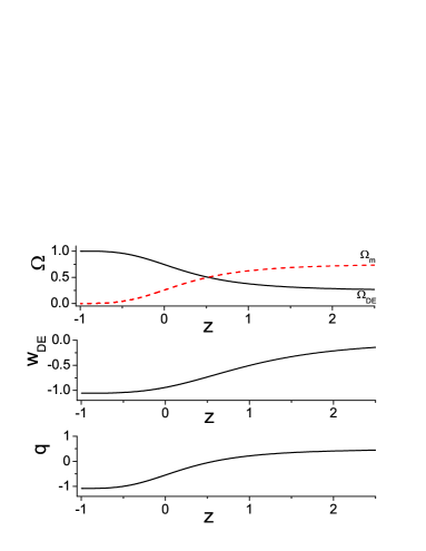
Figure 1: Upper graph: The evolution of the Ricci-Gauss-Bonnet holographic dark energy density parameter $\Omega_{DE}$ (black-solid) and of the matter density parameter $\Omega_{m}$ (red-dashed), as a function of the redshift $z$, for $\alpha=0.08$ and $\beta=0.001$, in units where $\kappa^{2}=1$. We have fixed the integration constant $x_{0}$ in (17) in order to obtain at present $\Omega_{DE}(z=0)\equiv\Omega_{DE0}\approx 0.68$. Middle graph: The evolution of the corresponding dark energy equation-of-state parameter $w_{DE}$. Lower graph: The evolution of the corresponding deceleration parameter $q$.

Let us now use the above expressions in order to examine the evolution of the Ricci-Gauss-Bonnet holographic dark energy density $\Omega_{DE}$ and equation-of-state $w_{DE}$ parameters in terms of the redshift $z$, given straightforwardly through $x\equiv\ln a=-\ln(1+z)$. In the upper graph of Fig. 1 we present $\Omega_{DE}(z)$ and $\Omega_{m}(z)=1-\Omega_{DE}(z)$, as they are given by the positive branch of (17). In the middle graph we depict the corresponding behavior of $w_{DE}(z)$ as it arises from (III). And in the lower graph we draw the deceleration parameter from (24). As we mentioned above, the integration constant $x_{0}$ in (17) has been chosen in order to obtain $\Omega_{DE}(z=0)\equiv\Omega_{DE0}\approx 0.68$ in agreement with observations Ade:2015xua . Finally, in the figures we have extended the evolution up to the far future, namely up to $z\rightarrow-1$ which corresponds to $t\rightarrow\infty$. As we observe, we can obtain the usual thermal history of the universe, with the transition from deceleration to acceleration happening at $z\approx 0.45$ as required, and in the future the universe tends asymptotically to a complete dark-energy dominated state.

We mention that according to (20), even if $\Omega_{DE}\rightarrow 1$ at $z\rightarrow-1$, the asymptotic value of $w_{DE}$ depends on the model parameters $\alpha$ and $\beta$. In order to observe this behavior more transparently, in Figs. 2 and 3 we present $w_{DE}(z)$ for various choices of $\alpha$ and $\beta$. In all cases the parameter $x_{0}$ in (17) has been chosen in order to obtain $\Omega_{DE}(z=0)\equiv\Omega_{DE0}\approx 0.68$, and additionally the specific pairs of $\alpha$ and $\beta$ have been chosen in order to obtain an early-time behavior of $\Omega_{DE}(z)$ in agreement with observations (i.e. similarly to Fig. 1).

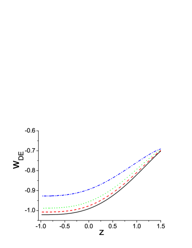
Figure 2: The evolution of the equation-of-state parameter $w_{DE}$ of the Ricci-Gauss-Bonnet holographic dark energy, as a function of the redshift $z$, for $\alpha=0.08$ and $\beta=0.005$ (black-solid), $\alpha=0.08$ and $\beta=0.007$ (red-dashed), $\alpha=0.08$ and $\beta=0.01$ (green-dotted), and $\alpha=0.08$ and $\beta=0.02$ (blue-dashed-dotted), in units where $\kappa^{2}=1$. We have fixed the integration constant $x_{0}$ in (17) in order to obtain at present $\Omega_{DE}(z=0)\equiv\Omega_{DE0}\approx 0.68$.

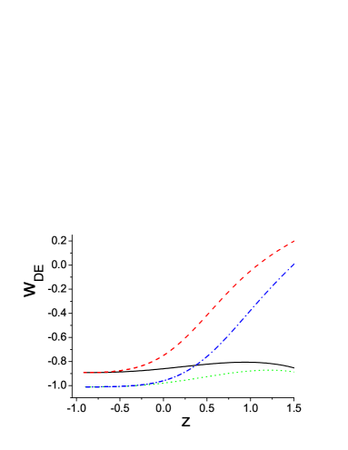
Figure 3: The evolution of the equation-of-state parameter $w_{DE}$ of the Ricci-Gauss-Bonnet holographic dark energy, as a function of the redshift $z$, for $\alpha=0.05$ and $\beta=0.1$ (black-solid), $\alpha=0.05$ and $\beta=-0.1$ (red-dashed), $\alpha=0.05$ and $\beta=0.08$ (green-dotted), and $\alpha=0.05$ and $\beta=-0.08$ (blue-dashed-dotted), in units where $\kappa^{2}=1$. We have fixed the integration constant $x_{0}$ in (17) in order to obtain at present $\Omega_{DE}(z=0)\equiv\Omega_{DE0}\approx 0.68$.

As we can see in Fig. 2, keeping $\alpha$ constant for increasing $\beta$ we obtain an increasing current (i.e. at $z=0$) and asymptotic future (i.e. at $z\rightarrow-1$) value of $w_{DE}$. Thus, for some parameter regions the dark energy can exhibit the phantom-divide crossing before or after the present time, for some other parameter regions it lies always in the quintessence regime, and for some other parameter regions $w_{DE}$ can asymptotically go to $-1$ i.e. the universe results in a de Sitter phase (one can see that Eq. (8) admits a late-time de Sitter solution if $1=12\alpha+2\sqrt{3}\beta$). For completeness we mention that one can have parameter regions in which $w_{DE}$ lies always in the phantom regime, and in some such cases the universe results to a Big Rip. Additionally, in Fig. 3 we can see that although the asymptotic value of $w_{DE}$ does not depend on the sign of $\beta$ (one can easily see by taking the approximation of (17) for $\Omega_{DE}\rightarrow 1$ and then of (III) that the resulting $w_{DE}$ depends only on $\beta^{2}$), its evolution depends significantly on that. Definitely, in order to thoroughly investigate the future behavior of the scenario at hand at late times, and extract the asymptotic solutions and their stability, one should apply dynamical system methods Copeland:1997et ; Bahamonde:2017ize , however such a detailed analysis lies beyond the scope of this work.

We note here that in Figs. 2 and 3 we desire to present the effects of the parameters $\alpha$ and $\beta$ on the cosmological behavior. If one wishes additionally to obtain $|w_{DE}+1|\lesssim 0.1$ over the redshift interval $z=[0,1.5)$ as it is favored by observations, then he should consider only e.g. the black-solid and green-dotted curves of 3. Definitely, the complete confrontation with the observed behavior can only be obtained using detailed data from Type Ia Supernovae (SN Ia), Baryon Acoustic Oscillations (BAO), Cosmic Microwave Background (CMB) shift parameter, and Hubble parameter observations, and perform the appropriate analysis.

At this point we should mention that for $\beta=0$, i.e. for the case of usual Ricci dark energy, the above expressions are significantly simplified. In particular, (17) can be inverted giving $\Omega_{DE}$ in an explicit form as

$$\Omega_{DE}|_{Ric}=\frac{e^{\frac{x}{3\alpha}+c_{1}}-3\alpha e^{x+3\alpha c_{1}}}{e^{\frac{x}{3\alpha}+c_{1}}-e^{x+3\alpha c_{1}}},$$ (25)

and then (12) leads to

$$H|_{Ric}=H_{0}\sqrt{\Omega_{m0}}e^{\frac{-3x}{2}}\left[\frac{(3\alpha-1)e^{x+3\alpha c_{1}}}{e^{\frac{x}{3\alpha}+c_{1}}-e^{x+3\alpha c_{1}}}\right]^{-1/2},$$ (26)

and therefore inserting these into (11) gives

$$\rho_{DE}|_{Ric}=\frac{3H_{0}^{2}\Omega_{m0}}{\kappa^{2}(3\alpha-1)}\left[e^{-c_{1}(3\alpha-1)}e^{\left(\frac{1}{3\alpha}-4\right)x}-3\alpha e^{-3x}\right],$$ (27)

which coincides exactly with the result of Gao:2007ep up to the re-definition of constants (the authors of that manuscript use a coupling $\alpha$ which is 6 times our $\alpha$ and they set $\kappa^{2}$ to $8\pi$). Finally, in this case (III), using also (16), is simplified to

$$w_{DE}|_{Ric}=\frac{1}{3\Omega_{DE}}-\frac{1}{\alpha}.$$ (28)

On the other hand, for $\alpha=0$ we obtain a pure Gauss-Bonnet holographic dark energy. In this case the solution is obtained from (17) setting $\alpha=0$, however although significantly simpler the resulting expression cannot be inverted. Nevertheless, (III), using also (16) can be greatly simplified, giving

$$w_{DE}|_{GB}=-\frac{1}{3\Omega_{DE}}\left(\frac{\Omega_{DE}^{2}}{12\beta^{2}}+1\right).$$ (29)

We close this section by investigating the above scenario under two extensions. The first is when we allow for an interaction between the Ricci-Gauss-Bonnet holographic dark energy and the dark-matter sector. The second is when we include also the radiation sector, in order to describe the whole thermal history of the universe.

• Interacting case

  In a general dark-energy scenario one may allow for an interaction between dark-energy and dark-matter sectors, since on one hand such an interaction cannot be excluded by theoretical arguments, and on the other hand it proves to lead to an alleviation of the so-called coincidence problem, namely why the density parameters of dark energy and dark matter are almost equal today although these sectors follow a completely different scaling during cosmological evolution Zimdahl:2001ar ; Chen:2008ft .

  In order to quantify the interaction we follow the standard procedure and we modify the conservation equations (9) and (19) as

  $$\dot{\rho}_{m}+3H(\rho_{m}+p_{m})=-Q$$ (30)

  $$\dot{\rho}_{DE}+3H(1+w_{DE})\rho_{DE}=Q,$$ (31)

  where $Q$ is a phenomenological descriptor of the interaction. Thus, $Q>0$ corresponds to energy transfer from the dark-matter sector to the dark-energy one, whereas $Q<0$ corresponds to transformation of dark energy to dark matter. Although the form of $Q$ can be chosen at will, a well-studied choice is to assume that $Q=\xi H\rho_{m}$, with $\xi$ a parameter, which has a reasonable justification since the interaction rate is indeed expected to be proportional to the energy density Zimdahl:2001ar ; Chen:2008ft .

  Let us now see how the Ricci-Gauss-Bonnet holographic dark energy cosmology will change in the presence of the above interaction term $Q$. Firstly, according to (30) the matter evolution will become

  $$\rho_{m}=\frac{\rho_{m0}}{a^{3+\xi}},$$ (32)

  and therefore (12) will become

  $$H=\frac{H_{0}\sqrt{\Omega_{m0}}}{\sqrt{a^{3+\xi}(1-\Omega_{DE})}}.$$ (33)

  Hence, (13) will extend to

  $$\dot{H}=-\frac{H^{2}}{2(1-\Omega_{DE})}\left[(3+\xi)(1-\Omega_{DE})-\Omega_{DE}^{\prime}\right],$$ (34)

  and then (14), (15) will read as

  $$R=-3H^{2}\left[1-\xi+\frac{\Omega_{DE}^{\prime}}{1-\Omega_{DE}}\right]$$ (35)

  $$G=12H^{4}\left[\frac{\Omega_{DE}^{\prime}}{1-\Omega_{DE}}-1-\xi\right].$$ (36)

  Thus, the differential equation (16) for $\Omega_{DE}$ extends to

  $$\Omega_{DE}=3\alpha\left[1\!-\!\xi\!+\!\frac{\Omega_{DE}^{\prime}}{1\!-\!\Omega_{DE}}\right]+2\sqrt{3}\beta\sqrt{\left|\frac{\Omega_{DE}^{\prime}}{1\!-\!\Omega_{DE}}\!-\!1-\!\xi\right|}.$$ (37)

  The analytical solution of the above differential equation, which generalizes (17) in the interacting case, writes as

  $$\!\!\!\!\!\!\!\!\!\!\!\epsilon_{\pm}\frac{\gamma_{+}}{\delta\zeta_{+}\sqrt{1+\xi}}\,\text{arctanh}\left(-\frac{\sqrt{6\alpha^{2}+\beta^{2}-\alpha\,\Omega_{DE}}}{\zeta_{+}}\right)$$

  $$\!\!\!\!\!\!\!\!\!\!\!\!-\epsilon_{\pm}\frac{\gamma_{-}}{\delta\zeta_{-}\sqrt{1+\xi}}\,\arctan\left(-\frac{\sqrt{6\alpha^{2}+\beta^{2}-\alpha\,\Omega_{DE}}}{\zeta_{-}}\right)$$

  $$\!\!\!\!\!\!\!\!\!\!\!\!-24\epsilon_{\pm}\frac{\beta}{\delta}\sqrt{6\alpha^{2}+\beta^{2}-\alpha}\,\text{arctanh}\left(\!\frac{\sqrt{6\alpha^{2}\!+\!\beta^{2}\!-\!\alpha\,\Omega_{DE}}}{\sqrt{6\alpha^{2}\!+\!\beta^{2}\!-\!\alpha}}\right)$$

  $$\!\!\!\!\!\!\!\!\!\!\!\!\!-\frac{\sqrt{3}[3\alpha^{2}(1-\xi)\!+\!2\beta^{2}\!-\!\alpha]}{\delta}$$

  $$\cdot\ln\left\{\frac{(1+\xi)[9\alpha^{2}(1+\xi)\!-\!12\beta^{2}\!-\!6\alpha\,\Omega_{DE}]\!+\!\Omega_{DE}^{2}}{(\Omega_{DE}-1)^{2}}\right\}$$

  $$\!\!\!\!\!\!\!\!\!\!\!\!\!\!-\frac{2[3\alpha(3\!+\!\xi)\!-\!1]\beta}{\delta\sqrt{1\!+\!\xi}}\,\text{arctanh}\!\left[\frac{\Omega_{DE}\!-\!3\alpha(1\!-\!\xi)}{2\sqrt{3}\beta\sqrt{1\!+\!\xi}}\right]\!=\!2\ln a\!+\!x_{0},\ \$$ (38)

  where $\epsilon_{\pm}=\pm 1$, but now with

  $$\!\!\!\gamma_{\mp}=2\left\{\mp 9\alpha^{3}(1-\xi^{2})+\beta^{2}\left(\pm 1+2\sqrt{3}\beta\sqrt{1+\xi}\right)\right.$$

  $$\ \ \ \ \ \ \ \ \ \ \left.\mp\alpha\beta\left[\pm 2\sqrt{3}\sqrt{1+\xi}+3\beta(5+3\xi)\right]\right.$$

  $$\ \ \ \ \ \ \ \ \ \ \left.+3\alpha^{2}\left[4\sqrt{3}\beta\sqrt{1+\xi}\pm(1+\xi)\right]\right\},$$

  $$\delta=\frac{1-6\alpha(1-\xi)+9\alpha^{2}(1-\xi)^{2}-12\beta^{2}(1+\xi)}{\sqrt{3}},$$

  $$\zeta_{\mp}=\sqrt{\mp 3\alpha^{2}(1+\xi)+2\sqrt{3}\alpha\beta\sqrt{1+\xi}\mp\beta^{2}}.$$ (39)

  Hence, as discussed above, $\xi>0$ corresponds to energy transfer from dark matter to dark energy, in which case the dark-energy domination will take place sooner, while $\xi<0$ corresponds to transformation of dark energy to dark matter, in which case the dark-energy epoch will arise later.

• Radiation inclusion

  As can be seen from the upper graph of Fig. 1, the matter energy density tends to 1 as $z$ grows, and one can easily verify that this behavior is maintained for the whole $z$-interval that is required for the correct description of the matter era (namely up to $z\sim 2000$). Nevertheless, since we have not explicitly included radiation, this matter-era will be maintained for larger $z$ too, and thus in order to stop it and obtain a radiation era in agreement with the thermal history of the universe, we must include radiation. In the following we provide the involved equations of the scenario of Ricci-Gauss-Bonnet holographic dark energy in the presence of the radiation sector, since this will allow us to describe the whole thermal history of the universe.

  In particular, considering

  $$\Omega_{r}\equiv\frac{\kappa^{2}}{3H^{2}}\rho_{r},$$ (40)

  the Friedmann equation (8) becomes $\Omega_{r}+\Omega_{m}+\Omega_{DE}=1$, which leads to

  $$H=\frac{H_{0}\sqrt{\Omega_{m0}}}{\sqrt{a^{3}(1-\Omega_{r}-\Omega_{DE})}}.$$ (41)

  Then (13) extends to

  $$\dot{H}=-\frac{H^{2}}{2(1\!-\!\Omega_{r}\!-\!\Omega_{DE})}\Bigl{[}3(1-\Omega_{r}-\Omega_{DE})\!-\!\Omega_{r}^{\prime}\!-\!\Omega_{DE}^{\prime}\Bigr{]},$$ (42)

  and similarly (14) and (15) become

  $$R=-3H^{2}\left[1+\frac{\Omega_{r}^{\prime}+\Omega_{DE}^{\prime}}{1-\Omega_{r}-\Omega_{DE}}\right]$$ (43)

  $$G=12H^{4}\left[\frac{\Omega_{r}^{\prime}+\Omega_{DE}^{\prime}}{1-\Omega_{r}-\Omega_{DE}}-1\right].$$ (44)

  Inserting these into (4) and then into (11) we obtain

  $$\Omega_{DE}=3\alpha\left[1+\frac{\Omega_{r}^{\prime}+\Omega_{DE}^{\prime}}{1-\Omega_{r}-\Omega_{DE}}\right]$$

  $$\ \ \ \ \ \ \ \ \ \,+2\sqrt{3}\beta\sqrt{\left|\frac{\Omega_{r}^{\prime}+\Omega_{DE}^{\prime}}{1-\Omega_{r}^{\prime}-\Omega_{DE}}-1\right|}.$$ (45)

  Finally, (21) and (22) are now extended to

  $$\frac{R^{\prime}}{3H^{2}}=3+2\left(\frac{\Omega_{r}^{\prime}+\Omega_{DE}^{\prime}}{1-\Omega_{r}-\Omega_{DE}}\right)-\frac{2(\Omega_{r}^{\prime}+\Omega_{DE}^{\prime})^{2}}{(1-\Omega_{r}-\Omega_{DE})^{2}}$$

  $$\ \ \ \ \ \ \ \ \ \ -\frac{\Omega_{r}^{\prime\prime}+\Omega_{DE}^{\prime\prime}}{1-\Omega_{r}-\Omega_{DE}}$$ (46)

  and

  $$\frac{|G^{\prime}|}{6H^{2}\sqrt{|G|}}=\frac{1}{\sqrt{3}(1-\Omega_{r}-\Omega_{DE})^{2}}\frac{1}{\sqrt{\left|\frac{\Omega_{r}^{\prime}+\Omega_{DE}^{\prime}}{1-\Omega_{r}-\Omega_{DE}}-1\right|}}$$

  $$\ \ \ \ \ \ \ \ \ \ \ \ \ \ \ \ \ \cdot\Big{\{}\Omega_{DE}^{\prime\prime}(1-\Omega_{r}-\Omega_{DE})+(\Omega_{r}^{\prime}+\Omega_{DE}^{\prime})^{2}$$

  $$\ \ \ \ \ \ \ \ \ \ \ \ \ \ \ \ \ \ \ \,-2\left[3(1-\Omega_{r}-\Omega_{DE})-\Omega_{r}^{\prime}-\Omega_{DE}^{\prime}\right]\cdot$$

  $$\ \ \ \ \ \ \ \ \ \ \ \ \ \ \ \ \ \ \ \ \ (\Omega_{r}^{\prime}+\Omega_{DE}^{\prime}+\Omega_{r}+\Omega_{DE}-1)\Big{\}},$$ (47)

  while (III) becomes

  $$w_{DE}=-1+\Omega_{DE}^{-1}\left\{\alpha\left[3+2\left(\frac{\Omega_{r}^{\prime}+\Omega_{DE}^{\prime}}{1-\Omega_{r}-\Omega_{DE}}\right)\right.\right.$$

  $$\left.\left.\ \ \ \ \ \ \ \ \ \ \ \ \ \ \ \ \ \ \ \ \ \ \ \ \ \ \ \ \ \ -\frac{2(\Omega_{r}^{\prime}+\Omega_{DE}^{\prime})^{2}}{(1-\Omega_{r}-\Omega_{DE})^{2}}\right.\right.$$

  $$\left.\ \ \ \ \ \ \ \ \ \ \ \ \ \ \ \ \ \ \ \ \ \ \ \ \ \ \ \ \ \ \,-\frac{\Omega_{r}^{\prime\prime}+\Omega_{DE}^{\prime\prime}}{1-\Omega_{r}-\Omega_{DE}}\right]$$

  $$-\frac{\beta}{\sqrt{3}(1-\Omega_{r}-\Omega_{DE})^{2}}\frac{1}{\sqrt{\left|\frac{\Omega_{r}^{\prime}+\Omega_{DE}^{\prime}}{1-\Omega_{r}-\Omega_{DE}}-1\right|}}$$

  $$\ \ \ \ \ \ \ \ \ \ \cdot\Big{\{}\Omega_{DE}^{\prime\prime}(1-\Omega_{r}-\Omega_{DE})+(\Omega_{r}^{\prime}+\Omega_{DE}^{\prime})^{2}$$

  $$\ \ \ \ \ \ \ \ \ \ \ \ \,-2\left[3(1-\Omega_{r}-\Omega_{DE})-\Omega_{r}^{\prime}-\Omega_{DE}^{\prime}\right]\cdot$$

  $$\left.\ \ \ \ \ \ \ \ \ \ \ \ \ \ (\Omega_{r}^{\prime}+\Omega_{DE}^{\prime}+\Omega_{r}+\Omega_{DE}-1)\Big{\}}\right\}.$$ (48)

  Contrary to (16), differential equation (45) does not accept an analytical solution, and thus one should elaborate it numerically.

  In Fig. 4 we present the evolution of the Ricci-Gauss-Bonnet holographic dark energy density parameter $\Omega_{DE}$, of the matter density parameter $\Omega_{m}$, and of the radiation density parameter $\Omega_{r}$, in the case where radiation is included in the scenario, imposing $\Omega_{DE0}\approx 0.68$, $\Omega_{m0}\approx 0.32$ and $\Omega_{r0}\approx 0.0001$ at present time, as required by observations. As we observe, we can obtain the thermal history of the universe, with the successive sequence of radiation, matter, and dark energy eras, before the universe result in complete dark-energy domination.

  

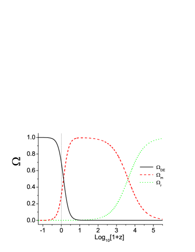
  Figure 4: The evolution of the Ricci-Gauss-Bonnet holographic dark energy density parameter $\Omega_{DE}$ (black-solid), of the matter density parameter $\Omega_{m}$ (red-dashed), and of the radiation density parameter $\Omega_{r}$ (green-dotted), as a function of the redshift $z$, for $\alpha=0.05$ and $\beta=0.12$ in units where $\kappa^{2}=1$, in the case where radiation is included in the scenario. We have imposed $\Omega_{DE}(z=0)\equiv\Omega_{DE0}\approx 0.68$, $\Omega_{m}(z=0)\equiv\Omega_{m0}\approx 0.32$, and $\Omega_{r}(z=0)\equiv\Omega_{r0}\approx 0.0001$ at present time, marked by the dotted vertical line.

IV Constraints from Big Bang Nucleosynthesis

As one can see from expression (7), Ricci-Gauss-Bonnet holographic dark energy is not necessarily zero at early times. Hence, apart from the basic phenomenological requirements imposed in the previous section, one should carefully examine the constraints that should be imposed on the scenario from Big Bang Nucleosynthesis (BBN). Hence, in this Section we examine the BBN constraints in detail.

The energy density of relativistic particles constituting the Universe is ${\displaystyle\rho_{r}=\frac{\pi^{2}}{30}g_{*}{{T}}^{4}}$, where $g_{*}\sim 10$ is the effective number of degrees of freedom and ${{T}}$ the temperature (in the Appendix we review the main features related to the BBN physics). The neutron abundance is computed via the conversion rate of protons into neutrons, namely

$$\lambda_{pn}({{T}})=\lambda_{n+\nu_{e}\to p+e^{-}}+\lambda_{n+e^{+}\to p+{\bar{\nu}}_{e}}+\lambda_{n\to p+e^{-}+{\bar{\nu}}_{e}}\,,$$

and its inverse $\lambda_{np}({{T}})$, and the relevant quantity is the total rate

$$\Lambda({{T}})=\lambda_{np}({{T}})+\lambda_{pn}({{T}})\,.$$ (49)

Explicit calculations of Eq. (49) (see (75) in the Appendix) give

$$\Lambda({{T}})=4A\,{{T}}^{3}(4!{{T}}^{2}+2\times 3!{\cal Q}{{T}}+2!{\cal Q}^{2})\,,$$ (50)

where ${\cal Q}=m_{n}-m_{p}$ is the mass difference of neutron and proton, and $A=1.02\times 10^{-11}$GeV^-4. The primordial mass fraction of ${}^{4}He$ can be estimated by making use of the relation kolb

$$Y_{p}\equiv\lambda\,\frac{2x(t_{f})}{1+x(t_{f})}\,,$$ (51)

where $\lambda=e^{-(t_{n}-t_{f})/\tau}$, with $t_{f}$ the time of the freeze-out of the weak interactions, $t_{n}$ the time of the freeze-out of the nucleosynthesis, $\tau$ the neutron mean lifetime given in (72), and $x(t_{f})=e^{-{\cal Q}/{{T}}(t_{f})}$ the neutron-to-proton equilibrium ratio. The function $\lambda(t_{f})$ is interpreted as the fraction of neutrons that decay into protons during the interval $t\in[t_{f},t_{n}]$. Deviations from the fractional mass $Y_{p}$ due to the variation of the freezing temperature ${{T}}_{f}$ are given by

$$\delta Y_{p}=Y_{p}\left[\left(1-\frac{Y_{p}}{2\lambda}\right)\ln\left(\frac{2\lambda}{Y_{p}}-1\right)-\frac{2t_{f}}{\tau}\right]\frac{\delta{{T}}_{f}}{{{T}}_{f}}\,,$$ (52)

where we have set $\delta{{T}}(t_{n})=0$ since ${{T}}_{n}$ is fixed by the deuterium binding energy torres ; Lambiase1 . The experimental estimations of the mass fraction $Y_{p}$ of baryon converted to ${}^{4}He$ during the Big Bang Nucleosynthesis are $Y_{p}=0.2476$ and $|\delta Y_{p}|<10^{-4}\,$ coc ; altriBBN1 . Inserting these into (52) one infers the upper bound on $\frac{\delta{{T}}_{f}}{{{T}}_{f}}$, namely

$$\left|\frac{\delta{{T}}_{f}}{{{T}}_{f}}\right|<4.7\times 10^{-4}\,.$$ (53)

During the BBN, at the radiation dominated era, the scale factor evolves as $a\sim t^{1/2}$, where $t$ is cosmic time. The Ricci-Gauss-Bonnet holographic dark energy density $\rho_{DE}$ is treated as a perturbation to the radiation energy density $\rho_{r}$. The relation between the cosmic time and the temperature is given by ${\displaystyle\frac{1}{t}\simeq\left(\frac{32\pi^{3}g_{*}}{90}\right)^{1/2}\frac{{T}^{2}}{M_{P}}}$ (or ${{T}}(t)\simeq(t/\text{sec})^{1/2}$MeV). Furthermore, we use the entropy conservation $S\sim a^{3}{{T}}^{3}=constant$. The expansion rate of the Universe is derived from (8), and can be rewritten in the form

$$H = H_{GR}^{(R)}\sqrt{1+\frac{\rho_{DE}}{\rho_{r}}}=H_{GR}+\delta H\,,$$ (54)

$$\delta H = \left(\sqrt{1+\frac{\rho_{DE}}{\rho_{r}}}-1\right)H_{GR}\,,$$ (55)

where $H_{GR}=\displaystyle{\sqrt{\frac{\kappa^{2}}{2}\rho_{r}}}$ ($H_{GR}$ is the expansion rate of the Universe in general relativity). Thus, from the relation $\Lambda=H$, one derives the freeze-out temperature ${{T}}={{T}}_{f}\left(1+\frac{\delta{{T}}_{f}}{{{T}}_{f}}\right)$, with ${T}_{f}\sim 0.6$ MeV (which follows from $H_{GR}\simeq q{{T}}^{5}$) and

$$\left(\sqrt{1+\frac{\rho_{DE}}{\rho_{r}}}-1\right)H_{GR}=5q{{T}}_{f}^{4}\delta{{T}}_{f}\,,$$ (56)

from which, in the regime $\rho_{DE}\ll\rho_{r}$, one obtains:

$$\frac{\delta{{T}}_{f}}{{{T}}_{f}}\simeq\frac{\rho_{DE}}{\rho_{r}}\frac{H_{GR}}{10q{{T}}_{f}^{5}}\,,$$ (57)

with $q=4!A\simeq 9.6\times 10^{-36}$GeV^-4.

Let us now investigate the bounds that arise from the BBN constraints, on the free parameters $\alpha$ and $\beta$ of the scenario of Ricci-Gauss-Bonnet holographic dark energy. These constraint will be determined using Eqs. (57) and (7). Assembling everything (we neglect the last two terms in the parenthesis of (75)) we find

$$\frac{\delta{{T}}_{f}}{{{T}}_{f}}\simeq\frac{16q^{2}}{\pi^{5}}\left(\frac{90}{\kappa^{2}g_{*}}\right)^{5/2}\left(\frac{T_{f}}{T_{0}}\right)^{8}H_{0}^{2}\Omega_{m0}^{2}\left(12\alpha+2\sqrt{3}\beta\right),$$ (58)

with ${{T}}_{0}$, $H_{0}$ and $\Omega_{m0}$ the current values of the CMB temperature, of the Hubble parameter and of the matter density parameter, respectively. Hence, using the bound (53) we finally find that

$$12\alpha+2\sqrt{3}\beta<2.53,$$ (59)

in units where $\kappa^{2}=1$. As we can see, the examples considered in the previous section, where prove to exhibit a cosmological behavior in agreement with observations, as well as the de Sitter solution condition, lie within the above bound.

V Conclusions

In this work we presented a model of holographic dark energy in which the Infrared cutoff is determined by both the Ricci scalar and the Gauss-Bonnet invariant. Such a construction has the significant advantage that the Infrared cutoff, and consequently the holographic dark energy density, does not depend on the future (such as in standard holographic dark energy versions) or the past (such as in agegraphic dark energy versions) evolution of the universe, but only on its current features. Additionally, it has the theoretical advantage that the Infrared cutoff is determined by invariants, whose role is fundamental in gravitational theories. Finally, following the usual approach in such theories, we allowed for more than one invariants of the same order to contribute.

In order to investigate the cosmological applications of the Ricci-Gauss-Bonnet holographic dark energy we first elaborated the equations and we resulted to a simple differential equation for the holographic dark energy density parameter $\Omega_{DE}$ in terms of the logarithm of the scale factor (which is straightforwardly related to the logarithm of the redshift), that accepts an analytical solution. Furthermore, we extracted the form of the holographic dark energy equation-of-state parameter $w_{DE}$ as a function of $\Omega_{DE}$, and thus resulting to its form as a function of the redshift.

The scenario of Ricci-Gauss-Bonnet holographic dark energy leads to interesting cosmological behavior, with enhanced capabilities due to the presence of two model parameters. First of all one can obtain the usual thermal history of the universe, with a dark-matter era followed by a dark-energy one, where the onset of acceleration takes place at $z\approx 0.45$ in agreement with observations, resulting in the future to a complete dark energy domination. The corresponding dark energy equation-of-state parameter can have a rich behavior, lying in the quintessence regime, in the phantom regime, or experiencing the phantom-divide crossing during the cosmological evolution. Moreover, its asymptotic value in the far future is determined by the model parameters, and can be quintessence-like, phantom-like, or be exactly equal to the cosmological-constant value $-1$. In the simple case where the contribution of the Gauss-Bonnet invariant is set to zero we re-obtained the results of usual Ricci dark energy, while in the case where the contribution of the Ricci invariant is set to zero, we obtained a “pure” Gauss-Bonnet holographic dark energy, where the various expressions are simplified.

In the case where radiation is included, one can describe the whole thermal history of the universe, namely the successive sequence of radiation, matter, and dark energy eras, before the universe result in complete dark-energy domination. Finally, examining in detail the constraints that arise from Big Bang Nucleosynthesis, we showed that in the above solutions the chosen model parameters satisfy the obtained bound.

We mention here that the resulting form of the Ricci-Gauss-Bonnet holographic dark energy contains terms depending on the Hubble function and its derivative. This might be similar to some particular models of the “running vacuum” classes Basilakos:2012ra ; George:2015lok ; Sola:2016jky ; Basilakos:2011wm , nevertheless the significant advantage is that in the present scenario they are justified under the holographic considerations using invariants, while in the former classes of models they are introduced by hand. Similarly, the scenario at hand is a sub-class of the general covariant generalized holographic dark energy, in which the Infrared cutoff is an arbitrary function of the Hubble function, the particle and future horizons, the cosmological constant, the universe age and their derivatives Nojiri:2017opc , however in the present approach it is a theoretically justified and well-defined sub-class.

We close this work by mentioning that there are additional investigations that need to be done before the scenario of Ricci-Gauss-Bonnet holographic dark energy can be considered as a successful candidate for the description of nature. One should use data from Type Ia Supernovae (SN Ia), Baryon Acoustic Oscillations (BAO), Cosmic Microwave Background (CMB) shift parameter, and Hubble parameter observations, in order to extract constraints on the parameters of the scenario. Additionally, he should perform a perturbation analysis and confront it with perturbation-related data such as CMB temperature and polarization, Large Scale Structure (LSS) and gravitational lenses. Furthermore, he should apply the dynamical system methods in order to reveal the global behavior of the scenario at late times, independently of the early- and intermediate- time evolutions. These necessary studies lie beyond the scope of this manuscript and are left for future investigations.

Appendix A Big Bang Nucleosynthesis

In this Appendix we briefly review the main features of Big Bang Nucleosynthesis (BBN) following kolb ; bernstein . As it is known, in the early Universe the primordial ${}^{4}He$ was formed at temperature ${{T}}\sim 100$ MeV. Protons and neutrons were maintained in thermal equilibrium due to the interactions

$$\nu_{e}+n \longleftrightarrow p+e^{-}$$ (60)

$$e^{+}+n \longleftrightarrow p+{\bar{\nu}}_{e}$$ (61)

$$n \longleftrightarrow p+e^{-}+{\bar{\nu}}_{e}\,.$$ (62)

The neutron abundance is estimated by computing the conversion rate of protons into neutrons $\lambda_{pn}({{T}})$, and its inverse $\lambda_{np}({{T}})$. Therefore, the weak interaction rates at suitably high temperature read as

$$\Lambda({{T}})=\lambda_{np}({{T}})+\lambda_{pn}({{T}})\,,$$ (63)

where the rate $\lambda_{np}$ is given by

$$\lambda_{np}=\lambda_{n+\nu_{e}\to p+e^{-}}+\lambda_{n+e^{+}\to p+{\bar{\nu}}_{e}}+\lambda_{n\to p+e^{-}+{\bar{\nu}}_{e}}\,.$$ (64)

Finally, the rate $\lambda_{np}$ is related to the rate $\lambda_{pn}$ as $\lambda_{np}({{T}})=e^{-{\cal Q}/{{T}}}\lambda_{pn}({{T}})$, with ${\cal Q}=m_{n}-m_{p}$ the mass difference of neutron and proton.

During the freeze-out stage, one can use the following approximations bernstein : (i) The temperatures of particles are the same, i.e. ${{T}}_{\nu}={{T}}_{e}={T}_{\gamma}={{T}}$. (ii) The temperature ${{T}}$ is lower than the typical energies $E$ that contribute to the integrals entering the definition of the rates (one can thus replace the Fermi-Dirac distribution with the Boltzmann one, namely $n\simeq e^{-E/{{T}}}$). (iii) The electron mass $m_{e}$ can be neglected with respect to the electron and neutrino energies ($m_{e}\ll E_{e},E_{\nu}$).

Having these in mind, the interaction rate corresponding to the process (60) is given by

$$d\lambda_{n+\nu_{e}\to p+e^{-}}=d\mu\,(2\pi)^{4}|\langle{\cal M}|^{2}\rangle W\,,$$ (65)

where

$$d\mu \equiv \frac{d^{3}p_{e}}{(2\pi)^{3}2E_{e}}\frac{d^{3}p_{\nu_{e}}}{(2\pi)^{3}2E_{\nu_{e}}}\frac{d^{3}p_{p}}{(2\pi)^{3}2E_{p}}\,,$$ (66)

$$W \equiv \delta^{(4)}({\cal P})n(E_{\nu_{e}})[1-n(E_{e})]\,,$$ (67)

$${\cal P} \equiv p_{n}+p_{\nu_{e}}-p_{p}-p_{e}\,,$$ (68)

$${\cal M} = \left(\frac{g_{w}}{8M_{W}}\right)^{2}[{\bar{u}}_{p}\Omega^{\mu}u_{n}][{\bar{u}}_{e}\Sigma_{\mu}v_{\nu_{e}}]\,,$$ (69)

$$\Omega^{\mu} \equiv \gamma^{\mu}(c_{V}-c_{A}\gamma^{5})\,,$$ (70)

$$\Sigma^{\mu} \equiv \gamma^{\mu}(1-\gamma^{5})\,.$$ (71)

In (69) we have used the condition $q^{2}\ll M_{W}^{2}$, where $M_{W}$ is the mass of the vector gauge boson $W$, with $q^{\mu}=p_{n}^{\mu}-p_{p}^{\mu}$ the transferred momentum. From expression (65) it follows that $\lambda_{n+\nu_{e}\to p+e^{-}}=A\,{{T}}^{5}I_{y}\,,$ where $A\equiv\frac{g_{V}+3g_{A}}{2\pi^{3}}\,,$ and where $I_{y}=\int_{y}^{\infty}\epsilon(\epsilon-{\cal Q}^{\prime})^{2}\sqrt{\epsilon^{2}-y^{2}}\,n(\epsilon-{\cal Q})[1-n(\epsilon)]d\epsilon,$ with $y\equiv\frac{m_{e}}{{{T}}}\,,\quad{\cal Q}^{\prime}=\frac{{\cal Q}}{{{T}}}$.

A similar calculation for the process (61) gives $\lambda_{e^{+}+n\to p+{\bar{\nu}}_{e}}=A\,{{T}}^{5}J_{y}\,,$ with $J_{y}=\int_{y}^{\infty}\epsilon(\epsilon+{\cal Q}^{\prime})^{2}\sqrt{\epsilon^{2}-y^{2}}\,n(\epsilon)[1-n(\epsilon+{\cal Q}^{\prime})]d\epsilon\,,$ which finally results to $\lambda_{e^{+}+n\to p+{\bar{\nu}}_{e}}=A\,{{T}}^{3}(4!{{T}}^{2}+2\times 3!{\cal Q}{{T}}+2!{\cal Q}^{2})\,.$

Lastly, for the neutron decay (62) one obtains

$$\tau=\lambda_{n\to p+e^{-}+{\bar{\nu}}_{e}}^{-1}\simeq 887\text{sec}\,.$$ (72)

Hence, in the calculation of (64) we can safely neglect the above interaction rate of the neutron decay, i.e. during the BBN the neutron can be considered as a stable particle.

The above approximations (i)-(iii) lead to bernstein

$$\lambda_{e^{+}+n\to p+{\bar{\nu}}_{e}}=\lambda_{n+\nu_{e}\to p+e^{-}}\,.$$ (73)

Thus, inserting (73) into (64), and then into (63), allows to derive the expression for $\Lambda({{T}})$, namely

$$\Lambda({{T}})\simeq 2\lambda_{np}=4\lambda_{e^{+}+n\to p+{\bar{\nu}}_{e}}\,,$$ (74)

which using the above expressions leads to

$$\Lambda({{T}})=4A\,{{T}}^{3}(4!{{T}}^{2}+2\times 3!{\cal Q}{{T}}+2!{\cal Q}^{2})\,.$$ (75)

References

- (1) P. J. E. Peebles and B. Ratra, Rev. Mod. Phys. 75, 559 (2003) [astro-ph/0207347].
- (2) E. J. Copeland, M. Sami and S. Tsujikawa, Int. J. Mod. Phys. D 15, 1753 (2006) [hep-th/0603057].
- (3) Y. F. Cai, E. N. Saridakis, M. R. Setare and J. Q. Xia, Phys. Rept. 493, 1 (2010) [0909.2776 [hep-th]].
- (4) S. ’i. Nojiri and S. D. Odintsov, eConf C 0602061, 06 (2006) Int. J. Geom. Meth. Mod. Phys. 4, 115 (2007) [hep-th/0601213].
- (5) S. Capozziello and M. De Laurentis, Phys. Rept. 509, 167 (2011) [1108.6266 [gr-qc]].
- (6) Y. F. Cai, S. Capozziello, M. De Laurentis and E. N. Saridakis, Rept. Prog. Phys. 79, no. 10, 106901 (2016) [1511.07586 [gr-qc]].
- (7) G. ’t Hooft, Salamfest 1993: 0284-296 [gr-qc/9310026].
- (8) L. Susskind, J. Math. Phys. 36, 6377 (1995) [hep-th/9409089].
- (9) E. Witten, Adv. Theor. Math. Phys. 2, 253 (1998) [hep-th/9802150].
- (10) R. Bousso, Rev. Mod. Phys. 74, 825 (2002) [hep-th/0203101].
- (11) W. Fischler and L. Susskind, [hep-th/9806039].
- (12) D. Bak and S. J. Rey, Class. Quant. Grav. 17, L83 (2000) [hep-th/9902173].
- (13) P. Horava and D. Minic, Phys. Rev. Lett. 85, 1610 (2000) [hep-th/0001145].
- (14) A. G. Cohen, D. B. Kaplan and A. E. Nelson, Phys. Rev. Lett. 82, 4971 (1999) [hep-th/9803132].
- (15) M. Li, Phys. Lett. B 603, 1 (2004) [hep-th/0403127].
- (16) S. Wang, Y. Wang and M. Li, [1612.00345 [astro-ph.CO]].
- (17) R. Easther and D. A. Lowe, Phys. Rev. Lett. 82, 4967 (1999) [hep-th/9902088].
- (18) N. Kaloper and A. D. Linde, Phys. Rev. D 60, 103509 (1999) [hep-th/9904120].
- (19) R. Horvat, Phys. Rev. D 70, 087301 (2004) [astro-ph/0404204].
- (20) Q. G. Huang and M. Li, JCAP 0408, 013 (2004) [astro-ph/0404229].
- (21) D. Pavon and W. Zimdahl, Phys. Lett. B 628, 206 (2005) [gr-qc/0505020].
- (22) B. Wang, Y. g. Gong and E. Abdalla, Phys. Lett. B 624, 141 (2005) [hep-th/0506069].
- (23) S. Nojiri and S. D. Odintsov, Gen. Rel. Grav. 38, 1285 (2006) [hep-th/0506212].
- (24) H. Kim, H. W. Lee and Y. S. Myung, Phys. Lett. B 632, 605 (2006) [gr-qc/0509040].
- (25) B. Wang, C. Y. Lin and E. Abdalla, Phys. Lett. B 637, 357 (2006) [hep-th/0509107].
- (26) M. R. Setare, Phys. Lett. B 642, 1 (2006) [hep-th/0609069].
- (27) M. R. Setare and E. N. Saridakis, Phys. Lett. B 671, 331 (2009) [0810.0645 [hep-th]].
- (28) M. R. Setare and E. N. Saridakis, Phys. Lett. B 670, 1 (2008) [0810.3296 [hep-th]].
- (29) Y. g. Gong, Phys. Rev. D 70, 064029 (2004) [hep-th/0404030].
- (30) E. N. Saridakis, Phys. Lett. B 660, 138 (2008) [0712.2228 [hep-th]].
- (31) M. R. Setare and E. C. Vagenas, Int. J. Mod. Phys. D 18, 147 (2009) [0704.2070 [hep-th]].
- (32) M. R. Setare and E. C. Vagenas, Phys. Lett. B 666, 111 (2008) [0801.4478 [hep-th]].
- (33) E. N. Saridakis, JCAP 0804, 020 (2008) [0712.2672 [astro-ph]].
- (34) E. N. Saridakis, Phys. Lett. B 661, 335 (2008) [0712.3806 [gr-qc]].
- (35) M. Jamil, E. N. Saridakis and M. R. Setare, Phys. Lett. B 679, 172 (2009) [0906.2847 [hep-th]].
- (36) Y. Gong and T. Li, Phys. Lett. B 683, 241 (2010) [0907.0860 [hep-th]].
- (37) M. Bouhmadi-Lopez, A. Errahmani and T. Ouali, Phys. Rev. D 84, 083508 (2011) [1104.1181 [astro-ph.CO]].
- (38) M. Malekjani, Astrophys. Space Sci. 347, 405 (2013) [1209.5512 [gr-qc]].
- (39) M. Khurshudyan, J. Sadeghi, R. Myrzakulov, A. Pasqua and H. Farahani, Adv. High Energy Phys. 2014, 878092 (2014) [1404.2141 [gr-qc]].
- (40) R. C. G. Landim, Int. J. Mod. Phys. D 25, no. 04, 1650050 (2016) [1508.07248 [hep-th]].
- (41) A. Pasqua, S. Chattopadhyay, K. A. Assaf and I. G. Salako, Eur. Phys. J. Plus 131, no. 6, 182 (2016).
- (42) A. Jawad, N. Azhar and S. Rani, Int. J. Mod. Phys. D 26, no. 04, 1750040 (2016).
- (43) B. Pourhassan, A. Bonilla, M. Faizal and E. M. C. Abreu, [1704.03281 [hep-th]].
- (44) X. Zhang and F. Q. Wu, Phys. Rev. D 72, 043524 (2005) [astro-ph/0506310].
- (45) M. Li, X. D. Li, S. Wang and X. Zhang, JCAP 0906, 036 (2009) [0904.0928 [astro-ph.CO]].
- (46) C. Feng, B. Wang, Y. Gong and R. K. Su, JCAP 0709, 005 (2007) [0706.4033 [astro-ph]].
- (47) X. Zhang, Phys. Rev. D 79, 103509 (2009) [0901.2262 [astro-ph.CO]].
- (48) J. Lu, E. N. Saridakis, M. R. Setare and L. Xu, JCAP 1003, 031 (2010) [0912.0923 [astro-ph.CO]].
- (49) S. M. R. Micheletti, JCAP 1005, 009 (2010) [0912.3992 [gr-qc]].
- (50) S. D. H. Hsu, Phys. Lett. B 594, 13 (2004) [hep-th/0403052].
- (51) R. G. Cai, Phys. Lett. B 657, 228 (2007) [0707.4049 [hep-th]].
- (52) H. Wei and R. G. Cai, Phys. Lett. B 660, 113 (2008) [0708.0884 [astro-ph]].
- (53) H. Wei and R. G. Cai, Eur. Phys. J. C 59, 99 (2009) [0707.4052 [hep-th]].
- (54) M. Jamil and E. N. Saridakis, JCAP 1007, 028 (2010) [1003.5637 [hep-th]].
- (55) C. Gao, X. Chen and Y. G. Shen, Phys. Rev. D 79, 043511 (2009) [0712.1394 [astro-ph]].
- (56) C. J. Feng and X. Z. Li, Phys. Lett. B 679, 151 (2009) [0904.2976 [hep-th]].
- (57) C. J. Feng and X. Z. Li, Phys. Lett. B 680, 355 (2009) [0905.0527 [astro-ph.CO]].
- (58) M. Suwa and T. Nihei, Phys. Rev. D 81, 023519 (2010) [0911.4810 [astro-ph.CO]].
- (59) M. H. Belkacemi, M. Bouhmadi-Lopez, A. Errahmani and T. Ouali, Phys. Rev. D 85, 083503 (2012) [1112.5836 [gr-qc]].
- (60) P. A. R. Ade et al. [Planck Collaboration], Astron. Astrophys. 594, A13 (2016) [1502.01589 [astro-ph.CO]].
- (61) E. J. Copeland, A. R. Liddle and D. Wands, Phys. Rev. D57 (1998) 4686, [gr-qc/9711068].
- (62) S. Bahamonde, C. G. Boehmer, S. Carloni, E. J. Copeland, W. Fang and N. Tamanini, [1712.03107].
- (63) W. Zimdahl and D. Pavon, Phys. Lett. B 521, 133 (2001) [astro-ph/0105479].
- (64) X. m. Chen, Y. g. Gong and E. N. Saridakis, JCAP 0904, 001 (2009) [0812.1117 [gr-qc]].
- (65) E.W. Kolb, M.S. Turner, The Early Universe , Addison Wesley Publishing Company, (1989).
- (66) D.F. Torres, H. Vucetich, A. Plastino, Phys. Rev. Lett. 79, 1588 (1997) [astro-ph/9705068].
- (67) G. Lambiase, Phys. Rev. D 72, 087702 (2005) [astro-ph/0510386].
- (68) A. Coc et al., Astrophys.J. 600 (2004) 544-552 [astro-ph/0309480].
- (69) K.A. Olive, E. Stillman, G. Steigman, Astrophys. J. 483, 788 (1997) [astro-ph/9611166].
- (70) S. Basilakos, D. Polarski and J. Sola, Phys. Rev. D 86, 043010 (2012) [1204.4806 [gr-qc]].
- (71) P. George and T. K. Mathew, Mod. Phys. Lett. A 31, no. 13, 1650075 (2016) [1511.02019 [gr-qc]].
- (72) J. Solà, A. Gómez-Valent and J. de Cruz Pérez, Astrophys. J. 836, no. 1, 43 (2017) [1602.02103 [astro-ph.CO]].
- (73) S. Basilakos, F. Bauer and J. Sola, JCAP 1201, 050 (2012) [1109.4739 [gr-qc]].
- (74) S. Nojiri and S. D. Odintsov, [1703.06372 [hep-th]].
- (75) J. Bernstein, L.S. Brown, G. Feinberg, Rev. Mod. Phys. 61, 25 (1989).