J. P. Lees
V. Poireau
V. Tisserand
Laboratoire d’Annecy-le-Vieux de Physique des Particules (LAPP), Université de Savoie, CNRS/IN2P3, F-74941 Annecy-Le-Vieux, France
E. Grauges
Universitat de Barcelona, Facultat de Fisica, Departament ECM, E-08028 Barcelona, Spain
A. Palano
INFN Sezione di Bari and Dipartimento di Fisica, Università di Bari, I-70126 Bari, Italy
G. Eigen
University of Bergen, Institute of Physics, N-5007 Bergen, Norway
D. N. Brown
Yu. G. Kolomensky
Lawrence Berkeley National Laboratory and University of California, Berkeley, California 94720, USA
M. Fritsch
H. Koch
T. Schroeder
Ruhr Universität Bochum, Institut für Experimentalphysik 1, D-44780 Bochum, Germany
C. HeartyabT. S. MattisonbJ. A. McKennabR. Y. SobInstitute of Particle Physics; University of British Columbiab, Vancouver, British Columbia, Canada V6T 1Z1
V. E. BlinovabcA. R. BuzykaevaV. P. DruzhininabV. B. GolubevabE. A. KravchenkoabA. P. OnuchinabcS. I. SerednyakovabYu. I. SkovpenabE. P. SolodovabK. Yu. TodyshevabBudker Institute of Nuclear Physics SB RAS, Novosibirsk 630090a, Novosibirsk State University, Novosibirsk 630090b, Novosibirsk State Technical University, Novosibirsk 630092c, Russia
A. J. Lankford
University of California at Irvine, Irvine, California 92697, USA
J. W. Gary
O. Long
University of California at Riverside, Riverside, California 92521, USA
A. M. Eisner
W. S. Lockman
W. Panduro Vazquez
University of California at Santa Cruz, Institute for Particle Physics, Santa Cruz, California 95064, USA
D. S. Chao
C. H. Cheng
B. Echenard
K. T. Flood
D. G. Hitlin
J. Kim
T. S. Miyashita
P. Ongmongkolkul
F. C. Porter
M. Röhrken
California Institute of Technology, Pasadena, California 91125, USA
Z. Huard
B. T. Meadows
B. G. Pushpawela
M. D. Sokoloff
University of Cincinnati, Cincinnati, Ohio 45221, USA
J. G. Smith
S. R. Wagner
University of Colorado, Boulder, Colorado 80309, USA
D. Bernard
M. Verderi
Laboratoire Leprince-Ringuet, Ecole Polytechnique, CNRS/IN2P3, F-91128 Palaiseau, France
D. BettoniaC. BozziaR. CalabreseabG. CibinettoabE. FioravantiabI. GarziaabE. LuppiabV. SantoroaINFN Sezione di Ferraraa; Dipartimento di Fisica e Scienze della Terra, Università di Ferrarab, I-44122 Ferrara, Italy
A. Calcaterra
R. de Sangro
G. Finocchiaro
S. Martellotti
P. Patteri
I. M. Peruzzi
M. Piccolo
M. Rotondo
A. Zallo
INFN Laboratori Nazionali di Frascati, I-00044 Frascati, Italy
S. Passaggio
C. Patrignani
Now at: Università di Bologna and INFN Sezione di Bologna, I-47921 Rimini, Italy
INFN Sezione di Genova, I-16146 Genova, Italy
H. M. Lacker
Humboldt-Universität zu Berlin, Institut für Physik, D-12489 Berlin, Germany
B. Bhuyan
Indian Institute of Technology Guwahati, Guwahati, Assam, 781 039, India
U. Mallik
University of Iowa, Iowa City, Iowa 52242, USA
C. Chen
J. Cochran
S. Prell
Iowa State University, Ames, Iowa 50011, USA
H. Ahmed
Physics Department, Jazan University, Jazan 22822, Kingdom of Saudi Arabia
A. V. Gritsan
Johns Hopkins University, Baltimore, Maryland 21218, USA
N. Arnaud
M. Davier
F. Le Diberder
A. M. Lutz
G. Wormser
Laboratoire de l’Accélérateur Linéaire, IN2P3/CNRS et Université Paris-Sud 11, Centre Scientifique d’Orsay, F-91898 Orsay Cedex, France
D. J. Lange
D. M. Wright
Lawrence Livermore National Laboratory, Livermore, California 94550, USA
J. P. Coleman
E. Gabathuler
D. E. Hutchcroft
D. J. Payne
C. Touramanis
University of Liverpool, Liverpool L69 7ZE, United Kingdom
A. J. Bevan
F. Di Lodovico
R. Sacco
Queen Mary, University of London, London, E1 4NS, United Kingdom
G. Cowan
University of London, Royal Holloway and Bedford New College, Egham, Surrey TW20 0EX, United Kingdom
Sw. Banerjee
D. N. Brown
C. L. Davis
University of Louisville, Louisville, Kentucky 40292, USA
A. G. Denig
W. Gradl
K. Griessinger
A. Hafner
K. R. Schubert
Johannes Gutenberg-Universität Mainz, Institut für Kernphysik, D-55099 Mainz, Germany
R. J. Barlow
Now at: University of Huddersfield, Huddersfield HD1 3DH, UK
G. D. Lafferty
University of Manchester, Manchester M13 9PL, United Kingdom
R. Cenci
A. Jawahery
D. A. Roberts
University of Maryland, College Park, Maryland 20742, USA
R. Cowan
Massachusetts Institute of Technology, Laboratory for Nuclear Science, Cambridge, Massachusetts 02139, USA
S. H. Robertson
Institute of Particle Physics and McGill University, Montréal, Québec, Canada H3A 2T8
B. DeyaN. NeriaF. PalomboabINFN Sezione di Milanoa; Dipartimento di Fisica, Università di Milanob, I-20133 Milano, Italy
R. Cheaib
L. Cremaldi
R. Godang
Now at: University of South Alabama, Mobile, Alabama 36688, USA
D. J. Summers
University of Mississippi, University, Mississippi 38677, USA
P. Taras
Université de Montréal, Physique des Particules, Montréal, Québec, Canada H3C 3J7
G. De Nardo
C. Sciacca
INFN Sezione di Napoli and Dipartimento di Scienze Fisiche, Università di Napoli Federico II, I-80126 Napoli, Italy
G. Raven
NIKHEF, National Institute for Nuclear Physics and High Energy Physics, NL-1009 DB Amsterdam, The Netherlands
C. P. Jessop
J. M. LoSecco
University of Notre Dame, Notre Dame, Indiana 46556, USA
K. Honscheid
R. Kass
Ohio State University, Columbus, Ohio 43210, USA
A. GazaM. MargoniabM. PosoccoaG. SimiabF. SimonettoabR. StroiliabINFN Sezione di Padovaa; Dipartimento di Fisica, Università di Padovab, I-35131 Padova, Italy
S. Akar
E. Ben-Haim
M. Bomben
G. R. Bonneaud
G. Calderini
J. Chauveau
G. Marchiori
J. Ocariz
Laboratoire de Physique Nucléaire et de Hautes Energies, IN2P3/CNRS, Université Pierre et Marie Curie-Paris6, Université Denis Diderot-Paris7, F-75252 Paris, France
M. BiasiniabE. ManoniaA. RossiaINFN Sezione di Perugiaa; Dipartimento di Fisica, Università di Perugiab, I-06123 Perugia, Italy
G. BatignaniabS. BettariniabM. CarpinelliabAlso at: Università di Sassari, I-07100 Sassari, Italy
G. CasarosaabM. ChrzaszczaF. FortiabM. A. GiorgiabA. LusianiacB. OberhofabE. PaoloniabM. RamaaG. RizzoabJ. J. WalshaINFN Sezione di Pisaa; Dipartimento di Fisica, Università di Pisab; Scuola Normale Superiore di Pisac, I-56127 Pisa, Italy
A. J. S. Smith
Princeton University, Princeton, New Jersey 08544, USA
F. AnulliaR. FacciniabF. FerrarottoaF. FerroniabA. PilloniabG. PireddaaINFN Sezione di Romaa; Dipartimento di Fisica, Università di Roma La Sapienzab, I-00185 Roma, Italy
C. Bünger
S. Dittrich
O. Grünberg
M. Heß
T. Leddig
C. Voß
R. Waldi
Universität Rostock, D-18051 Rostock, Germany
T. Adye
F. F. Wilson
Rutherford Appleton Laboratory, Chilton, Didcot, Oxon, OX11 0QX, United Kingdom
S. Emery
G. Vasseur
CEA, Irfu, SPP, Centre de Saclay, F-91191 Gif-sur-Yvette, France
D. Aston
C. Cartaro
M. R. Convery
J. Dorfan
W. Dunwoodie
M. Ebert
R. C. Field
B. G. Fulsom
M. T. Graham
C. Hast
W. R. Innes
P. Kim
D. W. G. S. Leith
S. Luitz
D. B. MacFarlane
D. R. Muller
H. Neal
B. N. Ratcliff
A. Roodman
M. K. Sullivan
J. Va’vra
W. J. Wisniewski
SLAC National Accelerator Laboratory, Stanford, California 94309 USA
M. V. Purohit
J. R. Wilson
University of South Carolina, Columbia, South Carolina 29208, USA
A. Randle-Conde
S. J. Sekula
Southern Methodist University, Dallas, Texas 75275, USA
M. Bellis
P. R. Burchat
E. M. T. Puccio
Stanford University, Stanford, California 94305, USA
M. S. Alam
J. A. Ernst
State University of New York, Albany, New York 12222, USA
R. Gorodeisky
N. Guttman
D. R. Peimer
A. Soffer
Tel Aviv University, School of Physics and Astronomy, Tel Aviv, 69978, Israel
S. M. Spanier
University of Tennessee, Knoxville, Tennessee 37996, USA
J. L. Ritchie
R. F. Schwitters
University of Texas at Austin, Austin, Texas 78712, USA
J. M. Izen
X. C. Lou
University of Texas at Dallas, Richardson, Texas 75083, USA
F. BianchiabF. De MoriabA. FilippiaD. GambaabINFN Sezione di Torinoa; Dipartimento di Fisica, Università di Torinob, I-10125 Torino, Italy
L. Lanceri
L. Vitale
INFN Sezione di Trieste and Dipartimento di Fisica, Università di Trieste, I-34127 Trieste, Italy
F. Martinez-Vidal
A. Oyanguren
IFIC, Universitat de Valencia-CSIC, E-46071 Valencia, Spain
J. AlbertbA. BeaulieubF. U. BernlochnerbG. J. KingbR. KowalewskibT. LueckbI. M. NugentbJ. M. RoneybR. J. SobieabN. TasneembInstitute of Particle Physics; University of Victoriab, Victoria, British Columbia, Canada V8W 3P6
T. J. Gershon
P. F. Harrison
T. E. Latham
Department of Physics, University of Warwick, Coventry CV4 7AL, United Kingdom
R. Prepost
S. L. Wu
University of Wisconsin, Madison, Wisconsin 53706, USA
L. Sun
Wuhan University, Wuhan 430072, China
Abstract
We measure the mass difference, , between the and the using the decay chain with . The data were recorded with the BABAR detector at center-of-mass energies at and near the resonance, and correspond to an integrated luminosity of approximately . We measure
.
We combine this result with a previous BABAR measurement of to obtain
.
These results are
compatible with and
approximately five times more precise than the Particle Data Group averages.
The difference
between the masses of the and mesons 111charge conjugation is
implied throughout this paper.,
,
is a key ingredient constraining calculations of symmetry
breaking due to differing and
quark masses
and electromagnetic interactions in
the frameworks of chiral perturbation theory Goity and Jayalath (2007)
and lattice QCD Horsley et al. (2014).
Its value is reported by the Particle Data Group (PDG) Patrignani et al. (2016)
to be .
The most precise direct measurement,
reported by the LHCb Collaboration, is
Aaij et al. (2013).
This was found by comparing the invariant mass distributions of
and
decays.
A more powerful constraint comes from the difference of measured
and mass difference distributions.
CLEO has previously reported
using
the decay chain with Bortoletto et al. (1992).
In the present paper we report a new measurement
of and
combine it with our previously measured
mass difference Lees et al. (2013a, b),
, using two decay modes and , to determine
with very high precision.
This analysis is based on a data set corresponding to an integrated
luminosity of approximately 468 recorded at, and 40 below,
the resonance Lees et al. (2013).
The data were collected with the BABAR detector at the PEP-II asymmetric
energy collider, located at the SLAC National Accelerator Laboratory.
The BABAR detector is described in detail
elsewhere Aubert et al. (2002, 2013).
The momenta of charged particles are measured with a combination of a
cylindrical drift chamber (DCH) and a 5-layer silicon vertex tracker (SVT),
both operating within the T magnetic field of a superconducting solenoid.
Information from a ring-imaging Cherenkov detector is combined with specific
ionization () measurements from the SVT and DCH to identify charged
kaon and pion candidates.
Electrons are identified, and photons from decays are measured, with a CsI(Tl)
electromagnetic calorimeter (EMC).
The return yoke of the superconducting coil is instrumented with tracking
chambers for the identification of muons.
We study the transition, using the
decay mode, to determine the difference between the and masses .
To extract , we fit the distribution of the difference between
the reconstructed and masses, .
The signal component in the fit
is a resolution function determined from
our Monte Carlo (MC) simulation of the detector response,
while the contaminations from background are accounted for
by a threshold function.
We suppress combinatorial backgrounds, and backgrounds with candidates from decays,
by requiring mesons produced in reactions
to have momenta in the center-of-mass frame greater than .
Decays
with
create backgrounds
when the daughter of the decay
replaces the in the decay
by mistake and the two have similar momenta.
To mitigate this problem,
events
are rejected if for either of the two .
The value of 160 is chosen to be very conservative in terms of
removing decays Lees et al. (2013a, b)
and causes almost no loss of
signal.
The decay chain is fitted subject to
geometric constraints at the production vertex and
the decay vertex, and to a kinematic constraint that the
laboratory momentum points back to the
luminous region whose horizontal, vertical, and longitudinal
RMS dimensions are about
6, 9, and 120 m, respectively
Aubert et al. (2002).
The -value from the fit is required to be
greater than 0.1%.
The “slow pion” from decay, denoted as ,
has a typical laboratory momentum
of 300 . All photons from decays have energies below 500 .
Their energy resolution is , and angular resolutions
are and mr
where
the resolutions
are measured with large uncertainties.
In the reconstruction,
we first require both photon energies to be above 60 , the total energy
to be greater than 200 , and the diphoton invariant mass to be between
120 and 150 (approximately around the nominal mass Patrignani et al. (2016)).
After the selection, each photon pair is kinematically fitted to the hypothesis of a originating from the event primary vertex,
and with the diphoton mass constrained to the nominal mass. This greatly improves the
reconstructed momentum resolution, and
therefore the resolution. The relative momentum resolution after the kinematic fit is 3%; this is still considerably worse than the approximately 0.5% relative momentum resolution.
Our MC simulation attempts to track run-by-run variations in
detector response.
The standard MC energy calibration method that accounts for energy loss in the
EMC differs from that used with real data.
This results in a reconstructed mass () peak
in MC events that peaks about 0.5 below the nominal mass for low energy
s.
In contrast, the peak value from the calibrated data events
generally coincides with the nominal value.
Therefore, we approximate the
neutral energy correction algorithm used in data by
rescaling
the reconstructed photon energies in MC
events by factors
depending on
photon energy and data-taking period Aubert et al. (2013).
While this improves the
data-MC agreement,
the reconstructed momentum in MC events
remains slightly biased when compared with its generated
value.
To account for this bias, we also rescale
the momentum in each MC
event by
approximately 0.2%,
depending on the diphoton opening angle.
In addition to improving the data-MC agreement
in peak positions and shapes of the
background-subtracted distributions, these MC corrections
substantially improve the agreement in kinematic distributions,
as described below.
Decay candidates are formed from well-measured tracks with
kaon or pion particle identification and with a
invariant mass within
1.86 and 1.88 (approximately
around the nominal mass Patrignani et al. (2016)).
This reduces background from random combinations of tracks,
especially from decays with a correctly
reconstructed ,
which will also peak in the
signal region of the distribution.
As in Ref. Lees et al. (2013a), we reject candidates with any daughter track for which the cosine of the polar angle
measured in the laboratory frame
is above 0.89; this criterion reduces the final sample by approximately 10%.
To further suppress peaking background events,
we use a likelihood variable to select candidates,
based on measured decay vertex separation from the primary vertex, and on
Dalitz-plot position.
This likelihood criterion rejects about 70%
of background events with incorrectly reconstructed , while retaining
about 77% of
signal events.
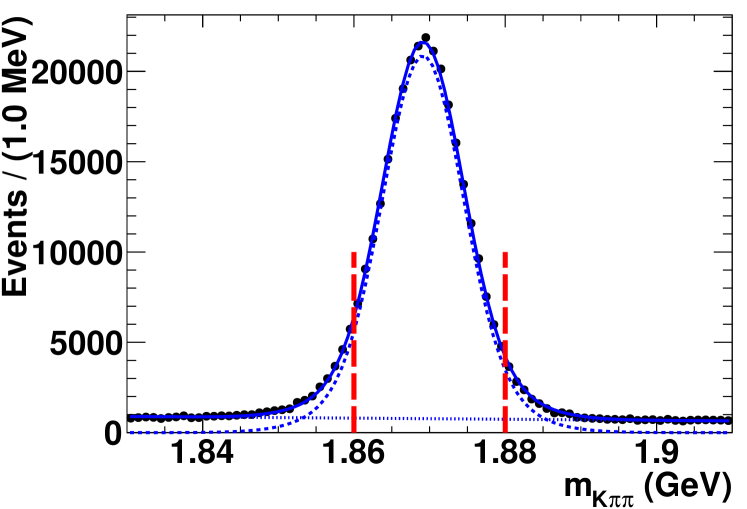
Figure 1 shows the distribution for
data events passing all selection criteria except for the requirement on .
For illustrative purposes, we fit the distribution by modeling the signal
with a sum of two Gaussian functions sharing a common mean, and random background events with a linear function.
After all selection criteria, the fraction of candidates with a correctly reconstructed ,
as estimated from the fit, is about 95%.
Figure 1: (color online) The reconstructed mass distribution
of real data, after all selection criteria except for the mass requirement,
which is marked by the two vertical dashed lines.
The result of the fit described in the text is superimposed
(solid line), together with the background (dotted line) and signal
(dashed line) components.
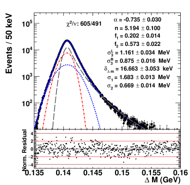
Figure 2: (color online) Left: fit to correctly reconstructed signal MC events.
Shown are the total fit (blue solid line), Crystal Ball function (gray long-dashed line), Gaussian (blue short-dashed line), and
two-piece normal distribution function
(red dash-dotted line).
The fitted signal shape parameters defined in Eq. 1 are also shown in the text box.
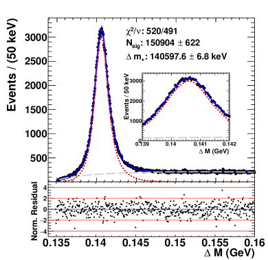
Right: fit to real data. Shown are the total fit (blue solid line), signal PDF (magenta short-dashed line), and background PDF (gray long-dashed line).
The inset shows the fit around the peak region.
The central value from the fit is later corrected
by the estimated fit bias.
Normalized residuals shown underneath both fit plots are defined as .
The value of is obtained from a fit to the
distribution in a two-step procedure as illustrated in Fig. 2 (a)
and (b). First, we model the resolution function
by fitting the distribution for correctly reconstructed
signal MC events
using an
empirically-motivated sum of three Gaussian or Gaussian-like probability density
functions (PDFs):
(1)
where and give the fractions for the composite PDFs of G (Gaussian), CB
(Crystal Ball 222M. J. Oreglia, Ph.D. thesis, Stanford University Report No. SLAC-R-236, 1980; J. E. Gaiser, Ph.D. thesis, Stanford University Report No. SLAC-R-255, 1982; T. Skwarnicki, Ph.D. thesis, Cracow Institute of Nuclear Physics Report No. DESY-F31-86-02, 1986.,
with and as two parameters to model the high mass tail), and BfG (
a two-piece normal distribution
with widths and on the left and right of , respectively).
The sum is therefore the common peak position of the three PDFs.
In the fit to the high-statistics MC sample (Fig. 2(a)),
is fixed at the generated value of 140.636 , and
is a measure of the possible bias induced by
our event selection procedure, or the chosen form for the resolution
function.
The fitted functional distribution provides a reasonably good description of
the data (with for a sample more than 7 times larger than the data).
The fit gives , with the uncertainty
from the limited size of our MC sample.
The fit results for the shape parameters are shown in Fig. 2(a);
and the full-width at half maximum (FWHM) of the resolution function is found to be about 2.1 ,
which is mainly due to
the resolution of the .
The second step (Fig. 2(b)) is an unbinned maximum-likelihood fit to real data
using the PDF from the first step to model signal, and a threshold function to model the combinatorial background Albrecht et al. (1990):
(2)
where , and is the slope parameter
which is allowed to vary in the fit.
We fix the end point at the nominal mass Patrignani et al. (2016) as the physical limit of .
In the data fit, we fix the bias , fractions , and CB tail parameters to the MC values from the first step,
while allowing the widths to be free in the fit to allow for differences between MC simulation and data.
Figure 2(b) presents the data and the fit, with the normalized residuals showing good data and fit agreement.
There are signal events,
the observed FWHM of the signal shape is about 2.0 ,
and
we determine
,
where the uncertainty is statistical only ().
A bias correction to this result will be discussed later.
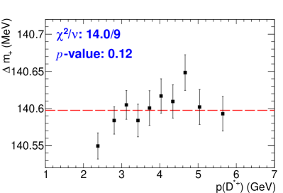
We estimate systematic uncertainties on from a variety of sources.
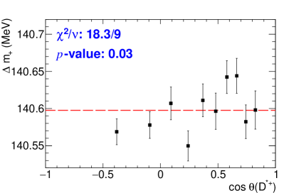
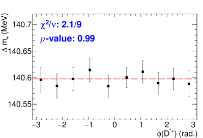
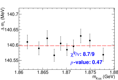
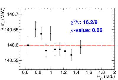
Separately, we study the dependence on the laboratory momentum , on the cosine of laboratory polar angle , on the laboratory azimuthal angle , on , and on the diphoton opening angle from , by collecting fit results for in 10 subsets of data with
roughly equal statistics for each parameter.
Furthermore,
we divide our data into four disjoint subsets of data-taking periods.
For the data fit in each subset, the value of
is determined separately from signal MC events with the same event selection criteria as for that subset.
This is
meant to expose possible detector response effects
that have not been modeled in the simulation.
We search for variations larger than those expected from statistical fluctuations based on a method similar to the PDG scale factor Lees et al. (2013b); Patrignani et al. (2016).
If the fit results from a given dependence study are compatible with a constant value, in the sense that ,
where is the number of degrees of freedom,
we assign no systematic uncertainty. In the case that , we ascribe an uncertainty of to account for unidentified detector effects.
We observe in the cases of ,
and (shown
in 333Additional plots are available through EPAPS Document No. E-PRLTAO-XX-XXXXX.
For more information on EPAPS, see http://www.aip.org/pubservs/epaps.html.).
Systematic uncertainties of
5.0 , 6.9 , and 6.1 are assigned for the
, , and
dependences, respectively, for which the -values for the null hypotheses are 0.12, 0.03, and 0.06.
The -values for the variations with azimuthal angle and mass are 0.99 and 0.47,
and no systematic uncertainties are assigned for these observations.
The five signal shape parameters , ,
, and , determined
from the fit to signal MC events (Fig. 2 (a)),
possess statistical uncertainties that are highly correlated.
We account for their uncertainties and correlations by
producing 100 sets of correlated random numbers of signal shape
parameters based on
the central values and the covariance matrix from the fit to signal
MC events. Then for each set, we rerun the data fit by fixing , ,
, and to the corresponding
random numbers in the set.
The distribution of the 100 fit values for
has a root mean square of 2.1 which is taken as
systematic uncertainty for the signal shape parameters.
To test whether our fit
procedure introduces a
bias on ,
we generate an ensemble of data sets with signal and background events
generated from appropriately normalized PDFs based on our nominal data fit.
The data sets are then fitted with exactly the same fit model as for real data (“pure pseudoexperiment”).
By performing 500 pseudoexperiments,
we collect
pulls, defined as the differences of fitted and input values normalized by the fitted errors. The
mean of the pulls is
,
while the root mean square is consistent with being unity.
We thus correct for the bias in our fit model
by adding
to the fit value of from the data, and assign a systematic uncertainty equal to half this bias correction
( ).
We perform another type of pseudoexperiment by fitting
to ensembles of data sets where signal and background events are
produced by randomly sampling the corresponding MC
events.
Background events from decays such as
with
misreconstructed as
produce small peaks in the signal region, but
the fit does not account for them explicitly.
The collected pulls show a mean fit bias consistent with that
found in our pure pseudoexperiments, and we assign no additional systematic
uncertainty related to peaking backgrounds.
To account for the systematic uncertainty due to
imperfect photon energy
simulation and calibration in the MC,
we rescale photon energies in
signal MC events
by and , and take the larger of the two variations in the peak position,
7.0, as the corresponding systematic uncertainty.
The values correspond to the difference between MC and
data mass peak positions after the nominal MC neutral energy corrections
are applied.
Because the MC and data distribution shapes differ,
aligning the peak positions does not produce equal mean values.
We also account for the associated
uncertainties on the momentum rescaling factors due to the limited size of our MC sample,
and find the related systematic uncertainty to be 0.5 .
Besides the systematic studies, we also perform a series of consistency checks that are not used to assess systematics
but rather to reassure us that the experimental approach and fitting technique behave reasonably.
We vary the upper limit of the fit range from its default position of 0.160 to a series
of values between 0.158 and 0.168 . Also, we vary the selection criteria
on the invariant masses and , as well as the Dalitz-plot based likelihood.
The resulting fit values of from all these checks are consistent.
Table 1: Assigned systematic errors from all considered sources.
Source
systematic [keV]
Fit bias
1.7
dependence
5.0
dependence
6.9
dependence
0.0
dependence
0.0
Diphoton opening angle dependence
6.1
Run period dependence
0.0
Signal model parametrization
2.1
EMC calibration
7.0
MC momentum rescaling
0.5
Total
All systematic uncertainties of are
summarized in Table 1; adding them in quadrature leads to a total
of 12.9 . After adding the fit bias of 3.4 keV,
our final result is
.
This result is consistent with the current world average of () ,
and about five times more precise.
Combining with the BABAR measurement of based
on the same data set, we obtain the meson mass difference of
.
This result is, as for , about a factor of five
more precise than the current world average, () .
Adding the statistical and systematic uncertainties in quadrature,
.
This can be compared with the corresponding values for the pion and kaon systems,
and Patrignani et al. (2016).
We are grateful for the excellent luminosity and machine conditions
provided by our PEP-II colleagues,
and for the substantial dedicated effort from
the computing organizations that support BABAR .
The collaborating institutions wish to thank
SLAC for its support and kind hospitality.
This work is supported by
DOE
and NSF (USA),
NSERC (Canada),
CEA and
CNRS-IN2P3
(France),
BMBF and DFG
(Germany),
INFN (Italy),
FOM (The Netherlands),
NFR (Norway),
MES (Russia),
MINECO (Spain),
STFC (United Kingdom),
BSF (USA-Israel).
Individuals have received support from the
Marie Curie EIF (European Union)
and the A. P. Sloan Foundation (USA).
References
Note (1)Charge conjugation is implied throughout this
paper.
Lees et al. (2013b)J. P. Lees et al. (BABAR Collaboration), Phys. Rev. D 88, 052003 (2013b), [Erratum: Phys. Rev. D 88,
079902 (2013)].
Lees et al. (2013)J. P. Lees et al. (BABAR Collaboration), Nucl. Instr. Meth.
Phys. Res., Sect. A 726, 203 (2013).
Aubert et al. (2002)B. Aubert et al. (BABAR Collaboration), Nucl. Instr.
Methods Phys. Res., Sect. A 479, 1 (2002).
Aubert et al. (2013)B. Aubert et al. (BABAR Collaboration), Nucl. Instr. Meth.
Phys. Res., Sect. A 729, 615 (2013).
Note (2)M. J. Oreglia, Ph.D. thesis, Stanford University Report No.
SLAC-R-236, 1980; J. E. Gaiser, Ph.D. thesis, Stanford University Report No.
SLAC-R-255, 1982; T. Skwarnicki, Ph.D. thesis, Cracow Institute of Nuclear
Physics Report No. DESY-F31-86-02, 1986.
Note (3)Additional plots are available through EPAPS Document No.
E-PRLTAO-XX-XXXXX. For more information on EPAPS, see
http://www.aip.org/pubservs/epaps.html.
I EPAPS Material
Figure 3: (color online) measurements
as functions of different properties:
(a) momentum magnitude ,
(b) polar angle ,
(c) azimuthal angle , (d) ,
and (e) opening angle .
In each plot we fit the results with a constant and the fitted with associated -value is shown in each plot.
The red dashed lines mark the central value from our nominal fit.