Statistical Properties of Photospheric Magnetic Elements Observed by SDO/HMI

Abstract

Magnetic elements of the solar surface are studied (using the 6173 Å Fe I line) in magnetograms recorded with the high$-$resolution Solar Dynamics Observatory$/$Helioseismic and Magnetic Imager (SDO$/$HMI). To extract some statistical and physical properties of these elements (e.g., filling factors, magnetic flux, size, lifetimes), the Yet Another Feature Tracking Algorithm (YAFTA), a region-based method, is employed. An area with 400${}^{\prime\prime}\times$400^′′ was selected to investigate the magnetic characteristics during the year 2011. The correlation coefficient between filling factors of negative and positive polarities is 0.51. A broken power law fit was applied to the frequency distribution of size and flux. Exponents of the power$-$law distributions for sizes smaller and greater than 16 arcsec² were found to be -2.24 and -4.04, respectively. The exponents of power$-$law distributions for fluxes smaller and greater than 2.63$\times$10¹⁹ Mx were found to be -2.11 and -2.51, respectively. The relationship between the size ($S$) and flux ($F$) of elements can be expressed by a power$-$law behavior in the form of $S\propto F~{}^{0.69}$. The lifetime and its relationship with the flux and size of quiet-Sun (QS) elements are studied during three days. The code detected patches with lifetimes of about 15 hours, which we call long-duration events. It is found that more than 95% of the magnetic elements have lifetimes of less than 100 minutes. About 0.05% of the elements were found with lifetimes of more than 6 hours. The relationships between the size ($S$), lifetime ($T$), and the flux ($F$) for patches in the QS, indicate the power$-$law relationships $S\propto T~{}^{0.25}$ and $F\propto T~{}^{0.38}$, respectively. Executing a detrended fluctuation analysis of the time series of new emerged magnetic elements, we find a Hurst exponent of 0.82, which implies long-range temporal correlation in the system.

1 Introduction

Undeniably, most of the solar atmospheric phenomena arise from photospheric magnetic fields, consisting of a wide range of sizes and strengths. The smallest magnetic features, with positive and negative polarities, known as “patches”, are well observed in magnetograms, which ubiquitously cover the solar surface with a scale-free distribution [(26)]. The field strength of the smallest elements can reach up to 1–2 kG, including sizes ranging from $10^{14}$ to $10^{16}$ cm² [(40)], with a typical flux of $10^{17}$–$10^{19}$ Mx (Hagenaar et al., 2003; Solanki, Inhester, and Sch$\ddot{u}$ssler, 2006; Priest, 2014). Fragments with a larger flux area are affected by four dominant processes – emergence, coalescence, fragmentation and cancellation (Close et al., 2005; DeForest et al., 2007), which can affect the event occurrence in the upper layers of the solar atmosphere. Studying their evolution, physical properties, and statistics, may give us a better understanding of the underlying physical processes.

Magnetic fields can appear as network regions elongated in intergranular lanes with an average of order 1 kG, or internetwork regions over the cell interiors in the quiet-Sun (QS), with an average of order 1 hG (Solanki, 1993; De Wijn et al., 2009; Gošić et al., 2014). Some of the statistical properties of magnetic elements were reported by Gošić et al., (2014, 2016), which quantify the physical parameters of magnetic features in the photosphere. Details on the magnetic field evolution in the solar atmosphere and photosphere can be found in Rieutord and Rincon (2010), Stein (2012), and Wiegelmann et al. (2014).

Because of the influence of the surface magnetic field on other events and its important role in energy release mechanisms, the relation between photospheric magnetic fields and other solar features (e.g., flares, and CMEs) were investigated in many articles (Schrijver and Title, 2003; Close et al., 2005; Wang et al., 2012; Gosain, 2012; Burtseva and Petrie, 2013; Honarbakhsh et al., 2016). On the other hand, some work paid attention to the statistical investigation of magnetic patches. A distribution of magnetic fluxes and areas relating to active regions and QS with different kinds of results were discussed in Schrijver et al. (1997a), Schrijver et al. (1997b), Abramenko & Longcope (2005), and Hagenaar et al. (2003). One of the latest work that studies magnetic fields in both active regions and QS for more than five decades, investigated the functional form of magnetic flux distribution based on a clumping algorithm [(26)]. They found that the flux of all features follow a power$-$law distribution with an exponent of approximately -1.85. Lamb et al. (2013) tracked 2$\times$10⁴ features in the QS to survey their birth (and death) during processes like cancellation, emergence, and fragmentation within a lifetime of an hour.

To analyze photospheric magnetic fields, solar space missions such as the Solar and Heliospheric Observatory (SOHO) and the Solar Dynamics Observatory (SDO) with their high spatial and temporal resolution, i.e., Michelson Doppler Imager [MDI; Scherrer et al., 1995] and Helioseismic and Magnetic Imager [HMI; Schou et al., 2012], respectively, provide a vast amount of information in the form of magnetogram images. To optimize the statistical data analysis techniques, it is necessary to develop and use automatic detection software (e.g., see Aschwanden, 2010; Javaherian et al., 2014; Arish et al., 2016). One of the robust and applicable algorithms is the code Yet Another Feature Tracking Algorithm (YAFTA) which is developed to segment and track small- and large-scale magnetic areas in magnetograms [(11)].

In a first step, in order to investigate magnetic patches in a wide range of scales, we employed the code YAFTA to segment (not to track) and extract the physical parameters (e.g., size distribution, filling factors, magnetic flux) of both negative and positive polarities within a large area in the magnetograms, taken from SDO$/$HMI during the year 2011. In addition to the flux distribution of magnetic elements, which has been discussed in Parnell et al. (2009), we focus on the other statistical parameters of patches, such as size and lifetime frequencies. Moreover, to find scaling laws between size, lifetime, and flux for magnetic features, we cropped smaller sizes of magnetograms in the QS with a much finer cadence of 45 s for a duration of three days.

The layout of this paper is as follows: the description of data sets is presented in Section 2. The results are presented and discussed in Section 3. Concluding remarks are given in Section 4.

2 Description of Data Sets

With the Helioseismic and Magnetic Imager (HMI), full solar disk images were observed in the Fe I absorption line at 6173 Å, with a resolution of 0.50$\pm$0.01 arcsec (equivalent to $3.58\times 10^{7}$ cm on the solar surface). Level-1 data are corrected for exposure time, dark current, gain, flat field, and cosmic-ray hits. We applied the code Yet Another Feature Tracking Algorithm (YAFTA) on the dataset recorded during the year 2011, from January 1 until December 31, taken at 13:00 UT with a cadence of one image per day.

The square area with a size of 400${}^{\prime\prime}\times$400^′′ at disk center is selected to ignore projection effects (e.g., McAteer et al., 2005; Alipour and Safari, 2015). This area is shown in Figure 1B (red box in Figure 1A). Both the size and flux distributions, the daily magnetic flux, and filling factors of polarities are extracted. In the next step, we focus on lifetimes, flux, and size in the quiet-Sun (QS). We downloaded level-1 HMI images for three days from 14 February to 16 February 2011 with a cadence of 45 s. Within 5750 consecutive frames, the area with the size of 100${}^{\prime\prime}\times$100^′′ is extracted from the solar equatorial region along the line of sight. This area is shown in Figure 1C (blue boxes in Figure 1A, and 1B).

The de-rotation procedure (drot_map.pro), available in the SSW/IDL package, is applied to coalign the images in the sequence. A subsonic filter was applied on our data cubes to remove the global solar p-mode oscillations for features with horizontal speeds faster than the 7 km s^-1 sound speed.

3 Results and Discussion

One of the robust software codes is Yet Another Feature Tracking Algorithm (YAFTA), which is improved by Deforest et al. (2007) and was employed in a number of studies (e.g., Burtseva and Petrie, 2013; Stangalini et al., 2013; Gošić et al., 2014). This software is accessible from the IDL library and computes properties of elements (magnetic flux with sign of polarity, size, etc.) and tracks them in a consecutive list of images. This study investigates statistical characteristics of magnetic elements during the year 2011 within a large area (Figure 1B), with a cadence of one image per day, covering 3 days (14–16 February) with a smaller area in the QS (Figure 1C), with a time step of 45 s between frames.

3.1 Statistical properties of magnetic elements during the year 2011

There are three kinds of algorithms for identifying structures of flux concentrations. In the clumping algorithm, pixels with fluxes higher than the determined threshold are considered as single feature [(25)]. In the downhill approach, after thresholding, one feature per local maximum region is assumed to be one identified magnetic element [Welsch and Longcope (2003)]. In this method, the number of detected patches is more than that of obtained by the clumping method. Curvature algorithm determines the boundaries as convex core around each local flux maximum [(16)]. In this method, the size of features decreases in comparison with the two previous approaches. It seems that downhill and clumping techniques produce better segmentation results than the curvature method [(11)].

We selected an area with $1.5\times 1.5$ arcsec² ($3\times 3$ pixels²), close to the value obtained by Parnell et al. (2009), as a minimum threshold in the grouping of pixels by the YAFTA’s downhill algorithm. The threshold of the magnetic field is selected to be 25 G (i.e., the code ignores pixels below this threshold in magnetograms). As mentioned in the previous section, to avoid projection effects, the area with a size of $400\times 400$ arcsec² is selected from solar equatorial regions (Figure 1A, red box). During the year 2011, the code detected 201,737 and 227,056 magnetic elements with positive and negative polarities, respectively.

The area filling factors of both positive and negative elements with their mean values are shown in Figure 2. The Pearson and Spearman correlation coefficients between filling factors of both time series were obtained with values of 0.51 and 0.29, respectively. The daily magnetic number of the two magnetic polarities is displayed in Figure 3. The size-frequency distribution of the magnetic elements is extracted (Figure 4). In order to minimize the difference between the histogram and an unknown density function, a data-based algorithm is used to find the optimum bin number in all histograms [(35)]. We fit a broken power law function to the frequency distribution of sizes. For sizes smaller than 16 arcsec², the exponent was obtained to be -2.24, and for the greater sizes, an exponent of -4.04. Moreover, the power law fit was applied to data points using the maximum likelihood estimator method [MLE; Clauset, Shalizi, and Newman, 2009]. Using MLE, the exponent of the fit for the whole range of data points yields the value of -2.71 $\pm$0.16. The maximum area of patches with negative polarity was found to have a size of 377 arcsec² in this analysis. The average of daily negative and positive flux with a yearly mean value of 2 $\times$ 10¹⁸ Mx is plotted in Figure 5.

The flux-frequency distribution of patches is plotted in Figure 6. A broken power law fit was applied to fluxes smaller, and greater than 2.63$\times$10¹⁹ Mx, yielding slope values of -2.11 and -2.51, respectively. Besides, by applying the MLE method on the whole range of the power law distribution, a power exponent of -2.15 $\pm$0.15 is obtained, which is close to the values in Parnell et al. (2009). The peak value of the flux is 1.52$\times$10²¹ Mx for the positive polarity group.

The scatter plots of the patch size versus flux, along with the mean values (red points) for each bin (0–0.1, 0.1–0.2 ($\times$10²⁰ Mx), etc.), are presented on a log$-$log scale in Figure 7. As we see in the scatter plot, more than 95$\%$ of the magnetic elements have fluxes less than 10²⁰ Mx, and patches with greater fluxes are more scattered in size. In most cases, element sizes are slightly larger for increasing elements fluxes. In order to find the relationship between the size ($S$) and flux ($F$), which is expressed in terms of arcsec² and 10²⁰Mx, respectively, we applied a linear fit (blue line) on the mean values of each bin on a log$-$log scale. It is found that the relationship between the size and flux can be expressed as $S\sim F^{a}$, with a best-fit parameter of $a=0.69$ (Figure 7).

3.2 Statistical properties of magnetic elements in the QS during 3 days

In the next step, we cropped areas in HMI$/$SDO images (Figure 1C) taken on 14$-$16 February 2011, and constructed a data cube with a cadence of 45 s, which includes 5750 sequential frames. We are interested in finding three consecutive days without a data gap in the quiet-Sun at solar disk center. We aim to study the statistical properties of magnetic elements (e.g., lifetimes, and relationships between lifetime, flux and size) in the QS from a large dataset. The total number of detected magnetic features is 185,150, and a fraction of 22,526 features did survive for more than one frame, which are labelled and tracked in time with the YAFTA’s match features algorithm. This algorithm is working based on making masks, using overlapping pixels in sequential images. The mean size of 22,526 events detected by YAFTA follows a power law size distribution with exponent of -4.50, as shown with a dashed line in a log$-$log scale in Figure 8. To compare filling factors of magnetic elements that appear in the QS (blue box in Figure 1A) with elements in the larger area (red box in Figure 1A), which is included the other regions than the QS, the filling factors of positive (red line) and negative (blue line) polarities are plotted in Figure 9. The Pearson and Spearman correlation coefficients are computed and were found to be 0.34 and 0.33, respectively. The MLE method is employed to find the power exponent of the lifetime-frequency of patches, shown as a power law fit (dashed line in Figure 10) on a log$-$log scale. The exponent is found to be -1.85. During these three days, one of the patches had a maximum lifetime of 876 minutes (see the electronic supplementary material (movie 1)), and 11 patches were found to have lifetimes greater than 6 hours. More than 90$\%$ of elements have lifetimes of less than 100 minutes. The time series of the flux and size for four patches with long duration lifetimes are shown in Figures 11 and 12, respectively. The histogram of flux for patches appearing in the QS is shown in Figure 13. By ignoring the left hand-side of the tail in the flux-frequency distribution, a linear fit with a slope of -3.31 is found for the distribution of mean fluxes on a log$-$log scale with more than 95$\%$ confidence. In this case, using the mean sizes and fluxes over the lifetime of a feature instead of the instantaneous values can make a difference in the obtained exponents. The peak flux amounts to 4.5 $\times 10^{17}$ Mx. In the QS, the maximum value for the flux belonging to a patch is 1.66$\times 10^{19}$ Mx.

The relationships between size, lifetime, and flux of patches in the QS (indicated with $S$, $T$, and $F$, respectively), are shown in the scatter plots as presented in Figures 14–16 on a log$-$log scale. In the same manner a scatter plot is shown in Figure 7, where the linear fits were applied to the mean values obtained for each bin. The results are as follows: The relation between mean size (arcsec²) of magnetic elements during their lifetimes and the lifetimes (minute) in the QS is defined by $S\simeq T^{c}$, where the fitting parameter $c$ is 0.25 (see the caption of Figure 14). The relation between the mean flux (10¹⁸ Mx) of magnetic elements during their lifetimes and the lifetimes (minute) in the QS is $F\simeq T^{e}$, where the fitting parameter $e$ is 0.38 (see the caption of Figure 15). The relation between mean size (arcsec²) and mean flux (10¹⁸ Mx) of magnetic features during their lifetimes in the QS is $S\simeq F^{g}$, where the fitting parameter $g$ is 0.64 (see the caption of Figure 16).

As we can see in Figure 14, features with different lifetimes have an excessive scatter in their sizes, but the clustering of points shows that most of the elements with smaller sizes (ranging from 2 to 8 arcsec²) have lifetimes of less than 100 minutes. In the same manner of Figure 14, in different ranges of patch lifetimes, there is an excessive scatter in the flux (Figure 15). But, as it can be seen in Figure 16, there is a clear relation between the size and flux. The size gradually grows up with increasing magnetic flux. The maximum value of size with 19.07 arcsec² belongs to a patch with a lifetime and flux of 171.5 minutes and 10 $\times$10¹⁸ Mx, respectively. The maximum value of the flux with about 11$\times$10¹⁸ Mx belongs to a patch with a lifetime and size of 289 minutes and 18 arcsec², respectively. The maximum value of lifetimes is 876 minutes, belonging to a patch with a size and flux of 16.67 arcsec² and 8.74$\times$10¹⁸ Mx, respectively.

Both the size and flux frequency distributions of the magnetic features (i.e., Figures 4, and 6) represent the fluctuations in the tail of the right-hand side of the histograms. It means that the statistical variations are larger than the bin count numbers. Newmann (2005) explained that this behavior is the characteristics of histograms that follow a power law distribution with an exponent larger than 2.

The detrended fluctuation analysis (DFA) is used to investigate the self-similarities in time series of new patches emerged in each sequence. In a time series, self-similarity for events in different time steps ($Y_{t}$) can be specified by the Hurst exponent ($H$).

$$Y_{at}=a^{-H}Y_{t},$$ (1)

where $a$ is a coefficient that determines any time later. If $H$ takes the values in the ranges of [0,0.5] and [0.5,1], we can say that the event has a long-term memory in its anti-correlated and positively correlated behavior, respectively. In the situation or $H$ = 0.5, there is an uncorrelated signal (white noise) in a time series [(22), (7)]. For exponents greater than unity the generalized Hurst exponent is introduced (for instance, refer to Heneghan and McDarby (2000)).

The task of DFA, which is introduced by Peng et al. (1994), is fitting a line $(a_{j}x+b_{j})$ for each cumulative time series $C_{i,j}$. The cumulative time series is defined as data series of components summation in each step over time. If the time series with length $L$ is broken down into $M$ subwindows with length $N$, the average of the mean square fluctuation for a whole of time series is given as

$$F(N)=\frac{1}{M}\sum_{j=1}^{M}\sqrt{\left(\frac{1}{N}\sum_{i=1}^{N}(C_{i,j}-a_{j}i-b_{j})^{2}\right)}.$$ (2)

Using the value of all subwindows $F(N)$ versus $N$, frequently expressed on a log$-$log scale, the Hurst exponent is evaluated [(2)].

The value of the Hurst exponent for the time series of all newly emerged magnetic features during three days is found to be 0.82 (Figure 17). The value shows that there is a long-term memory (auto-correlation) between different parts of the time series. The systems with long-term correlations can be described by small parts of the whole of system.

4 Conclusions

The automatic method Yet Another Feature Tracking Algorithm (YAFTA) for segmentation and tracking of photospheric magnetogram features taken by the Helioseismic and Magnetic Imager (HMI) was used to study statistical properties of magnetic elements. A statistical study of elements during the year 2011 shows a correlation coefficient of higher than 0.5 between filling factors of positive and negative polarities. The slope values of size-frequency distributions play an important role in small magnetic elements on the solar surface. The flux-frequency distribution follows a power law with a slope of about -2.15 $\pm$0.15, closely corresponding to the value found by Parnell et al. (2009). A few percent of the difference in the result may be caused by the spatial resolution of instruments and the employed method for identifying flux concentrations. The broken power law fits of both size and flux distributions illustrate that probably two different regimes govern the evolution of photospheric the magnetic elements. It is found that the relationship between size ($S$) and flux ($F$) of magnetic elements can be expressed as

$$S\propto F~{}^{0.69}.$$ (3)

Then, we focused on the statistical properties of patches in the QS during three days with a cadence of 45 s. Among the patches that survived more than one time during the analyzed sequence of images, more than 95% of the elements have lifetimes of less than 100 minutes. Moreover, 11 patches (about 0.05% of elements) were found to have lifetimes more than 6 hours and one of them lasted about 15 hours; the remaining 0.45% have lifetimes ranging from 100 to 360 minutes. The power law slopes are consistent with the following relationships between size ($S$), flux ($F$) and lifetimes ($T$) of elements in the QS as follows:

$$S\propto F~{}^{0.64},~{}~{}~{}~{}~{}S\propto T~{}^{0.25},~{}~{}~{}~{}~{}F\propto T~{}^{0.38}.$$ (4)

The exponents obtained from these relationships (between size $S$, flux $F$, and lifetimes $T$) describe scaling laws between the observed correlated quantities, as it is also evident from the Figures 15 and 16. According to Aschwanden (2015), deviations from ideal power-law distributions can originate from three natural effects, such as truncation effects, incomplete sampling of the smallest events below some threshold, or contamination by event-unrelated backgrounds. Since most sampled data are subject to a detection threshold (of their sizes for instance), the deviations from ideal power-laws can be explained by such data truncation effects.

The power law exponents of most distributions of self-organized criticality phenomena are consistent with power law-like distributions. Suppose that the frequency distributions of two variables, $x$ and $y$, follow the power-law function as $N(x)\sim x^{-\alpha_{x}}$ and $N(y)\sim y^{-\alpha_{y}}$, one can directly derive the relationship between the two variables $x$ and $y$. The correlation between $x$ and $y$ can be expressed by $y\sim x^{\beta}$. If the value of $\beta$ approaches unity, the variables $x$ and $y$ are proportional to each other. The exponent $\beta$ can be obtained by performing a linear regression fit to the logarithmic quantities $log(x)$ versus $log(y)$, as we indicate in the scatter plots shown in Figures 7, 14, 15, and 16.

To test the consistency between the power law coefficients obtained from the scatter plots (shown in relations 3 and 4), the following relation is used [(5)]

$$\beta=\frac{\alpha_{x}-1}{\alpha_{y}-1}.$$ (5)

As it can be seen in Figures 4 and 6, during the year 2011, the power law indices $\alpha_{{}_{{F}}}$ and $\alpha_{{}_{{S}}}$, which are extracted from histograms, were found to be 2.15 and 2.71, respectively. According to Figures 8, 10, and 13, the extracted values (in the quiet Sun) for the power law indices $\alpha_{{}_{{F}}}$, $\alpha_{{}_{{S}}}$, and $\alpha_{{}_{{T}}}$ are 3.31, 4.50, and 1.85, respectively. Using the power indices and Equation (5), the corresponding correlations are as follows:

$$S\propto F~{}^{0.67},~{}~{}~{}S_{{}_{\rm{QS}}}\propto F_{{}_{\rm{QS}}}~{}^{0.66},~{}~{}~{}S_{{}_{\rm{QS}}}\propto T_{{}_{\rm{QS}}}~{}^{0.24},~{}~{}~{}F_{{}_{\rm{QS}}}\propto T_{{}_{\rm{QS}}}~{}^{0.36}.$$ (6)

It can be seen that these values are in agreement with values presented by relations 3 and 4.

The evaluation of the Hurst exponent for time series of newly emerged magnetic elements on each day signifies that there is a correlation between various parts of the signal, which corresponds to the case of long-term memory. In other words, the self-similarity in the system (called fractal dimensionality) occurs at a higher level. So, a small fraction of the system can contain the information of the whole system [(5)], which is typical for scale-free parameters. It suggests that the system of solar magnetic features can be classified as a self-organized criticality system, representing scale-invariance characteristics of events with the ability of tuning itself as the system evolves.

In future work, we intend to extract all these statistical parameters from active regions and coronal holes when they appear in the solar equatorial region. Studying and comparing statistical properties of patches appearing in the network and internetwork magnetic elements, using both magnetograms and continuum intensity images taken by HMI (for example refer to Yousefzadeh et al., 2016), will be the focus of another project. Also, we are working on simulations of time series of magnetic elements, to study the evolution of their flux and size based on the obtained parameters and Monte-Carlo methods. These simulated time series will then be compared with observations using classifiers.

Acknowledgement

The authors acknowledge the YAFTA group: C. E. DeForest, H. J. Hagenaar, D. A. Lamb, C. E. Parnell, and B. T. Welsch for making YAFTA results publicly available.

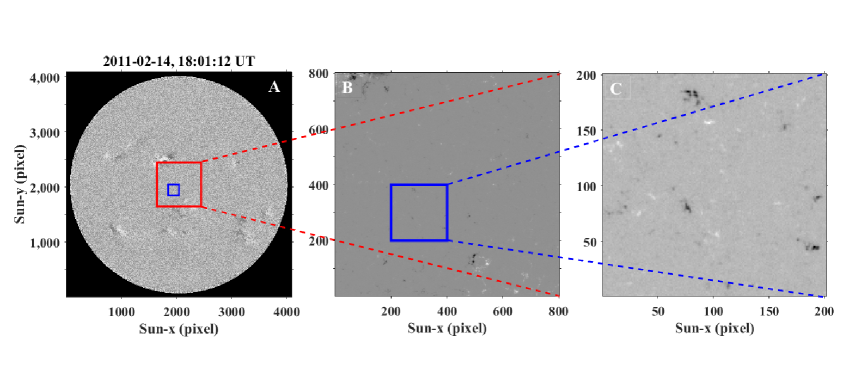
Figure 1.: The SDO$/$HMI full-disk magnetogram of the Sun recorded on 14 February 2011 (18:01:12 UT)(A). The cutout image with area of $400\times 400$ arcsec² (B) from the solar equatorial region is selected to extract physical parameters of positive and negative elements (such as size distributions, flux distributions, and filling factors) during the year 2011 with a cadence of one image per day. An image tile with area of $100\times 100$ arcsec² (C) is cropped from all images to investigate physical parameters of the magnetic elements especially their lifetimes for three days (14$-$16 February 2011) in the QS with a time lag of 45 s between frames.

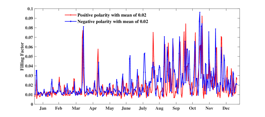
Figure 2.: Filling factors (area) of positive (red) and negative (blue) polarities (elements) are plotted from January 1 until December 31, 2011. The Pearson and Spearman correlations between these time series are 0.51 and 0.29, respectively.

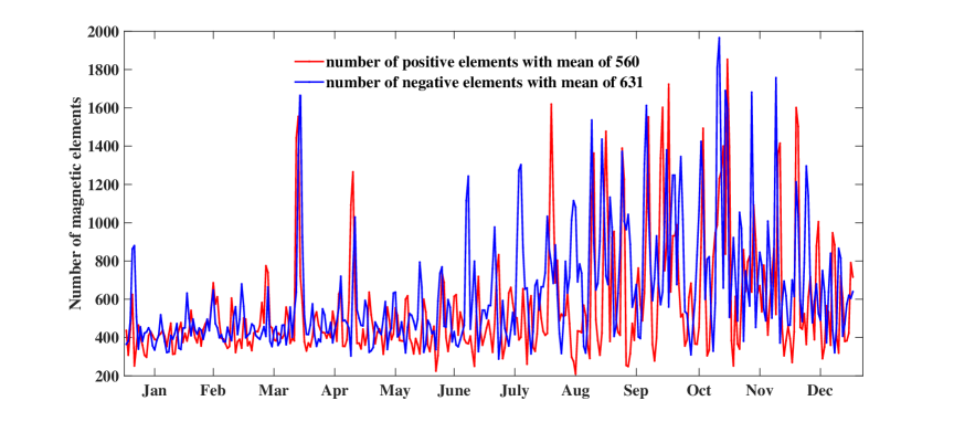
Figure 3.: Daily number of positive (red) and negative (blue) elements are shown from January 1 until December 31, 2011.

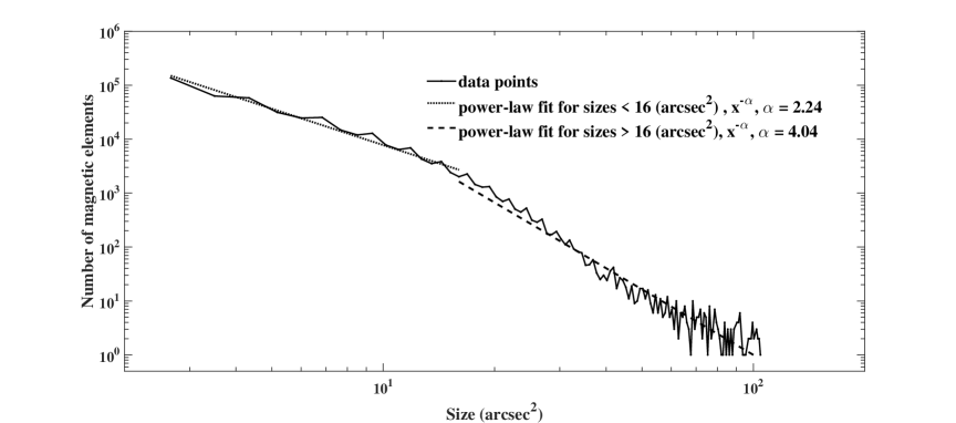
Figure 4.: Size-frequency distributions of unsigned magnetic elements are drawn in log$-$log scale. A broken double linear fits representing power-law exponents is fitted. For sizes smaller and greater than 16 arcsec², the exponents were obtained -2.24 and -4.04, respectively. Running the MLE method on the size-frequency distribution represented that the exponent of power-law fit for the whole range of sizes is equal to -2.71.

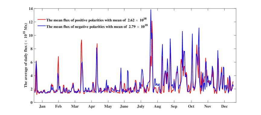
Figure 5.: Daily average flux of positive (red) and negative (blue) elements are shown from January 1 until December 31, 2011.

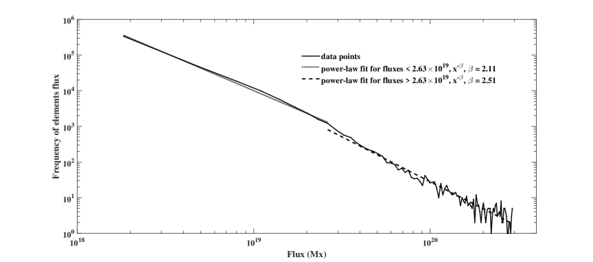
Figure 6.: Histogram of polarities flux with their broken linear fits for fluxes smaller than 2.63$\times$10¹⁹ Mx (the dotted line) and for fluxes greater than 2.63$\times$10¹⁹ Mx(the dashed line) in log$-$log scale. The exponents of the two ranges are equal to -2.11 and -2.51, respectively. Exerting the MLE method on the whole range of flux frequencies gives the value of -2.15 for power-law exponent.

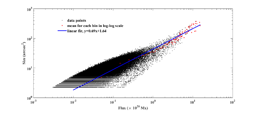
Figure 7.: Relationship between the size of patches (arcsec²) and their flux (Mx) in log$-$log scale. The mean values for each bin (0 -– 0.1, 0.1 –- 0.2 $(\times 10^{20}$ Mx), etc.) for magnetic elements are shown as red points. The blue solid line displays the linear fit, $\log(S)=a\log(F)+b$ with $a$ = 0.69 $\pm$ 0.06 and $b$ = 1.64 $\pm$ 0.04 with 95$\%$ confidence level in fitting.

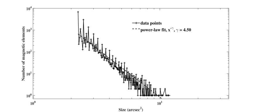
Figure 8.: The distribution of mean size of the polarities during their life in the QS are plotted in log$-$log scale. According to the MLE method, the dashed line shows a power-law exponent of fitting with value of -4.50.

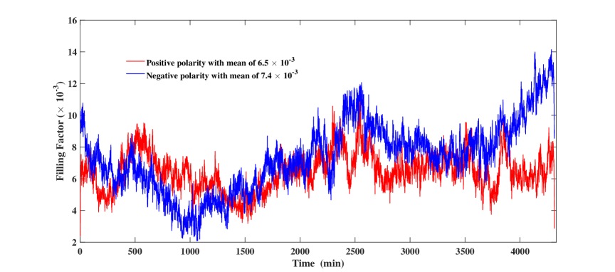
Figure 9.: Filling factors (area) of positive (red) and negative (blue) polarities of magnetic elements are displayed for each minute during three days (14$-$16 February). The Pearson and Spearman correlations between these time series are about 0.34 and 0.33, respectively.

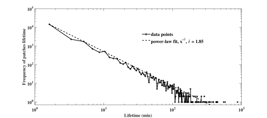
Figure 10.: Histogram of patches lifetime and its linear fit (the dashed line) with the slope of -1.85 extracted from the MLE method. The maximum lifetime is obtained to be 876 minutes, and 11 patches were found to have lifetimes greater than 6 hours.

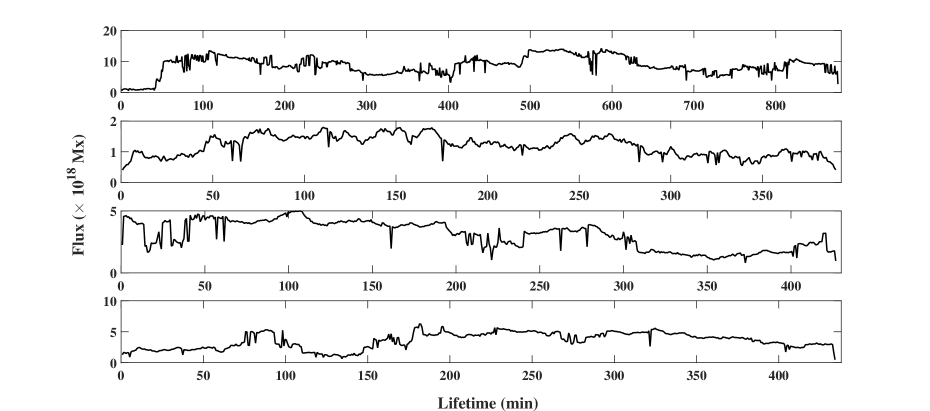
Figure 11.: The flux variations of four patches with lifetimes more than 6 hours.

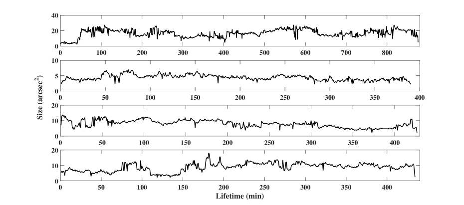
Figure 12.: The size variations of the same four patches shown in figure 11 during their lifetimes.

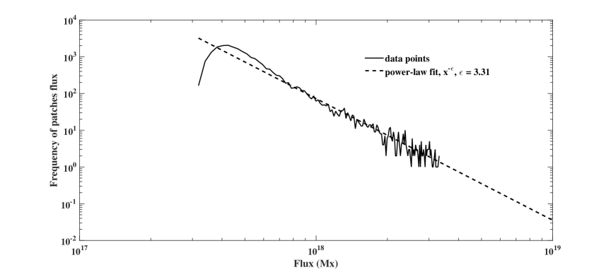
Figure 13.: The distribution of mean flux of the magnetic elements during their life in the QS are plotted in log$-$log scale. According to the MLE method, the dashed line shows a power-law exponent of fitting with value of -3.31.

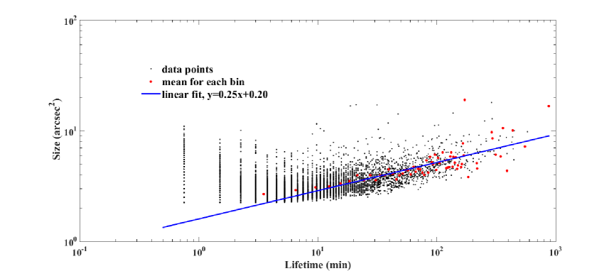
Figure 14.: Relationship between mean size of the patches (arcsec²) and their lifetime (min) appeared in the QS is shown in log$-$log scale. The mean values for each bin (0 -– 1, 1 –- 2 (min), etc.) for elements are indicated by red points. The blue solid line displays the linear fit, $\log(S)=c\log(T)+d$ with $c$ = 0.25 $\pm$ 0.06 and $d$ = 0.20 $\pm$ 0.1 with 95$\%$ confidence level in fitting.

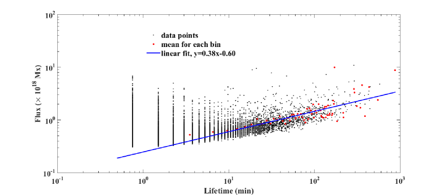
Figure 15.: Relationship between mean flux of the patches (Mx) and their lifetime (min) appeared in the QS is shown in log$-$log scale. The mean values for each bin (0 -– 1, 1 –- 2 (min), etc.) for elements are indicated by red points. The blue solid line displays the linear fit, $\log(F)=e\log(T)+f$ with $e$ = 0.38 $\pm$ 0.09 and $f$ = -0.60 $\pm$ 0.17 with 95$\%$ confidence level in fitting.

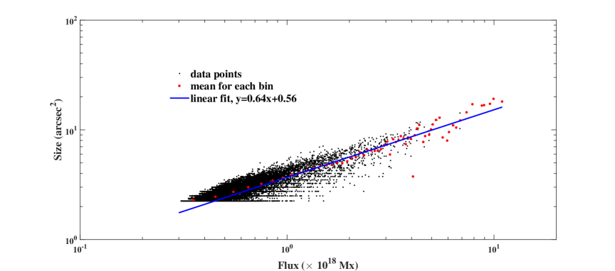
Figure 16.: Relationship between mean flux of the patches (Mx) and their mean size (arcsec²) during their lifetimes appeared in the QS is shown in log$-$log scale. The mean values for each bin (0 -– 0.1, 0.1 –- 0.2 ($\times 10^{18}$ Mx), etc.) for elements are indicated by red points. The blue solid line displays the linear fit, $\log(S)=g\log(F)+h$ with $g$ = 0.64 $\pm$ 0.06 and $h$ = 0.56 $\pm$ 0.04 with 95$\%$ confidence bounds.

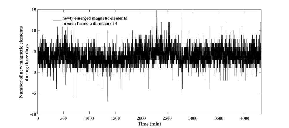
Figure 17.: The time series of new magnetic elements appeared in each magnetogram for three-day data with a cadence of 45 s are shown. The average of newly emerged magnetic elements in each frame is equal to 4 elements. The value of Hurst exponent extracted by DFA method is equal to 0.82.

References

- (1) Abramenko, V.I., Longcope, D.W.: 2005, ApJ, 619, 1160
- (2) Alipour, N., Safari, H.: 2015, ApJ807, 175
- (3) Arish, S., Javaherian, S., Safari, H., Amiri, A.: 2016, Sol. Phys.291, 1209
- (4) Aschwanden, M.J.: 2010, Sol. Phys.262, 235
- (5) Aschwanden, M.J.: 2011, Self-Organized Criticality in Astrophysics, Springer, Praxis Publishing, Chichester, UK.
- (6) Aschwanden, M.J.: 2015, ApJ814, 19A
- (7) Buldyrev, S.V., Goldberger, A.L., Havlin, S., et al.: 1995, Phys. Rev. E, 51, 5084
- (8) Burtseva, O., Petrie, G.: 2013, Sol. Phys.283, 429B
- (9) Clauset, A., Shalizi, C.R., Newman, M.E.J.: 2009, SIAM Review 51(4), 661
- (10) Close, R.M., Parnell, C.E., Longcope, D.W., Priest, E.R.: 2005, Sol. Phys.231, 45C
- (11) DeForest C.E., Hagenaar, H.J., Lamb, D.A., Parnell, C.E., Welsch, B.T.: 2007, ApJ666, 576
- (12) de Wijn, A.G., Stenflo, J.O., Solanki, S.K., Tsuneta, S.: 2009, Space Sci. Rev. 144, 275
- (13) Gošić, M., Bellot Rubio L.R., Orozco Suárez, D., Katsukawa, Y., del Toro Iniesta J.C.: 2014, ApJ797, 49
- (14) Gošić, M., Bellot Rubio L.R., del Toro Iniesta J.C., Orozco Suárez, D., Katsukawa, Y.: 2016, ApJ820, 35G
- (15) Gosain, S.: 2012, ApJ749, 85
- (16) Hagenaar, H.J., Schrijver, C.J., Title, A.M., Shine, R. A.: 1999, ApJ511, 932
- (17) Hagenaar, H.J., Schrijver, C.J., Title, A.M.: 2003, ApJ584, 1107
- (18) Heneghan, C., McDarby, G.: 2000, Phys. Rev. E 62, 6103
- (19) Honarbakhsh, L., Alipour, N., Safari, H.: 2016, Sol. Phys.291, 941H
- (20) Javaherian, M., Safari, H., Amiri, A., Ziaei, S.: 2014, Sol. Phys.289, 3969 J
- (21) Lamb, D.A., Howard, T.A., DeForest, C.E., Parnell, C.E., Welsch, B.T.: 2013, ApJ774, 127
- (22) Mandelbrot, B.B., Van Ness, J.W.: 1968, SIAMR 10, 422
- (23) McAteer, R.T.J., Gallagher, P.T., Ireland, J., Young, C.A.: 2005, Sol. Phys.228, 55
- (24) Newman, M.E.J.: 2005, ConPh, 46, 323
- (25) Parnell, C.E.: 2002, MNRAS335, 389
- (26) Parnell, C.E., DeForest, C.E., Hagenaar, H.J., Johnston, B.A., Lamb, D.A., Welsch, B.T.: 2009, ApJ698, 75
- (27) Peng, C.K., Buldyrev, S.V., Havlin, S., Simons, M., Stanley, H.E., Goldberger, A.L.: 1994, Phys. Rev. E 49, 1685
- (28) Priest, E.R.: 2014, Magnetohydrodynamics of the Sun, Cambridge University Press
- (29) Rieutord, M., Rincon, F.: 2010, Living Rev. Sol. Phys. 7, 2
- (30) Scherrer, P.H., Bogart, R.S., Bush, R.I., Hoeksema, J.T., Kosovichev, A.G., Schou, J., et al.: 1995, Sol. Phys.162, 129
- (31) Schou, J., Scherrer, P. H., Bush, R. I., Wachter, R., Couvidat, S., Rabello-Soares, M. C., et al.: 2012, Sol. Phys.275, 229
- (32) Schrijver, C.J., Title, A.M., Hagenaar, H.J., Shine, R.A.: 1997a, Sol. Phys.175, 329
- (33) Schrijver, C.J., Title, A.M., van Ballegooijen, A.A., Hagenaar, H.J., Shine, R.A.: 1997b, ApJ487, 424
- (34) Schrijver, C.J., Title, A.M.: 2003, ApJ597, 165
- (35) Shimazaki, H., Shinomoto, S.: 2007, Neural Computation 19, 1503
- (36) Solanki, S.K.: 1993, Space Sci. Rev.63, 1
- (37) Solanki, S.K., Inhester, B., Schssler, M.: 2006, Rep. Prog. in Phys. 69, 563
- (38) Stein, R.F.: 2012, Living Rev. Sol. Phys. 9, 4
- (39) Stangalini, M., Solanki, S.K., Cameron, R., Martínez, V.: 2013, A&A554, A115
- (40) Stenflo, J. O.: 1973, Sol. Phys.32, 41S
- (41) Wang, S., Liu, C., Liu, R., Deng, N., Liu, Y., Wang, H.: 2012, ApJ745, L17
- Welsch and Longcope (2003) Welsch, B.T., Longcope, D.W.: 2003, ApJ588, 620
- (43) Wiegelmann, T., Thalmann, J. K., Solanki, S. K.: 2014, A&A Rev., 22, 78
- (44) Yousefzadeh, M., Safari, H., Attie, R., Alipour, N.: 2016, Sol. Phys.291, 29Y