Simultaneous Precision Spectroscopy of pp, ⁷Be, and pep Solar Neutrinos with Borexino Phase-II

Abstract

We present the simultaneous measurement of the interaction rates $R_{pp}$, $R_{\rm{Be}}$, $R_{pep}$ of $pp$, ⁷Be, and $pep$ solar neutrinos performed with a global fit to the Borexino data in an extended energy range (0.19 – 2.93) MeV with particular attention to details of the analysis methods. This result was obtained by analyzing 1291.51 days of Borexino Phase-II data, collected after an extensive scintillator purification campaign. Using counts per day (cpd)/100 ton as unit, we find $R_{pp}$ = 134 $\pm$ 10 (stat) ${}^{+6}_{-10}$ (sys), $R_{Be}$ = 48.3 $\pm$ 1.1 (stat) ${}^{+0.4}_{-0.7}$ (sys); and $R_{pep}^{\rm{HZ}}$ = $2.43\pm 0.36\,({\it stat})^{+0.15}_{-0.22}\,({\it sys})$ assuming the interaction rate $R_{\rm{CNO}}$ of CNO-cycle solar neutrinos according to the prediction of the high metallicity Standard Solar Model, and $R_{pep}^{\rm{LZ}}$ = $2.65\pm 0.36\,({\it stat})^{+0.15}_{-0.24}\,({\it sys})$ according to that of the low metallicity model.

An upper limit $R_{\rm{CNO}}$ $<$ 8.1 cpd/ 100 ton (95% C.L.) is obtained by setting in the fit a constraint on the ratio $R_{pp}/R_{pep}$ (47.7 $\pm$ 0.8 cpd/100 ton or 47.5 $\pm$ 0.8 cpd/100 ton according to the high or low metallicity hypothesis).

I Introduction

Solar neutrinos produced in electron flavour $(\nu_{e})$ in fusion reactions occurring in the Sun provide a unique and direct way to study the interior of our star. The main contribution to the solar luminosity ($\sim$99%) comes from reactions belonging to the $pp$ chain, while the CNO cycle is expected to play a sub-dominant role Fowler (1958); *bib:TheoryB.

The solar neutrino $(\nu)$ spectrum, as predicted by the Standard Solar Model (SSM) Bahcall (2005); Vinyoles et al. (2017), is dominated by the low-energy neutrinos produced in the primary $pp$ reaction (E_ν $<$ 0.42 MeV) and it extends up to $\sim$18.8 MeV (maximum energy of the $hep$ $\nu$s). It also features two mono-energetic lines from ⁷Be $\nu$s (E_ν = 0.384 MeV and 0.862 MeV) and one mono-energetic line from $pep$ $\nu$s (E_ν = 1.44 MeV). Neutrinos from the CNO cycle are expected to have a continuous energy spectrum extending up to 1.74 MeV. The spectrum of ⁸B $\nu$s is also continuous and it ends up at about 16.5 MeV.

The 50-year-long experimental effort to study solar neutrinos Anselmann et al. (1992); *bib:GallexB; *bib:Sage; *bib:Homestake; *bib:Kamiokande; *bib:SK; *bib:SNO; Bellini et al. (2011a) has been extremely rewarding both in terms of solar physics, by confirming the SSM predictions Vinyoles et al. (2017), and in terms of particle physics, by giving a substantial contribution to the discovery of neutrino flavour oscillations Kajita and McDonald (2015), Jr. and Koshiba (2002). The present-day precision spectroscopy of solar neutrinos aims at studying the details of their energy spectrum by disentangling the contributions from the different reactions ($pp$ chain $\nu$s, namely $pp$, ⁷Be, $pep$, ⁸B, and $hep$ $\nu$s, and CNO cycle $\nu$s).

On the one hand, if the SSM predictions of solar fluxes $\phi$ are assumed, measuring the solar neutrino interaction rates $R$ for different reactions helps to pin down the electron-flavour neutrino survival probability $P_{ee}$ for different energies (that is the probability that $\nu_{e}$s do not undergo flavor oscillations while travelling from their Sun production point to the detector). Consequently, it probes the predictions of the MSW-LMA model Wolfenstein (1978); *bib:MSWB and can set constraints on possible deviations, e.g. due to non–standard interactions (NSI) Friedland et al. (2004); *bib:NSIb; *bib:NSIc; *bib:NSId.

On the other hand, if the neutrino oscillation parameters are assumed, the study of specific components of the solar neutrino spectrum can cross-check the SSM predictions. In particular, the experimental determination of the fluxes $\phi$ of ⁷Be, ⁸B or CNO neutrinos, which are the most sensitive ones to the solar metallicity (the abundance of the elements heavier than He in the Sun), can help to settle the question of high (HZ) versus low (LZ) metallicity Vinyoles et al. (2017).

The Borexino experiment has recently reported a comprehensive measurement of the solar neutrino spectrum from the whole $pp$ nuclear fusion chain in the energy range of (0.19 – 16) MeV. These results are presented in Agostini et al. (2018a) together with their physical implications. They include the updated values of the neutrino survival probability $P_{ee}$ as a function of the neutrino energy, the first direct measurement of the ratio $\mathcal{R}$ between the ³He $+$ ⁴He ($pp$-II) and the ³He $+$ ³He ($pp$-I) branches of the $pp$ chain obtained by combining our results on the ⁷Be and $pp$ $\nu$s, and finally a preference for the HZ-metallicity choice in the SSM.

In this paper we present the details of the analysis of the data belonging to the lowest part of the energy spectrum which extends from 0.19 to 2.93 MeV. This Low Energy Region (LER) is used to extract the interaction rates $R_{pp}$, $R_{{\rm Be}}$, $R_{pep}$, as well as to set the limit on $R_{{\rm CNO}}$. The analysis of the data from the so-called High Energy Region (HER) from 3.2 to 16 MeV, where our sensitivity to ⁸B $\nu$s is maximized and from 11 to 20 MeV energy region, in which the first Borexino limit on $hep$ $\nu$s is set, is discussed in Agostini et al. (2017a).

While our previous measurements of the $pp$ Bellini et al. (2014a), ⁷Be Bellini et al. (2011a), $pep$  Bellini et al. (2012), and ⁸B Bellini et al. (2010) $\nu$s were obtained separately by analyzing data in restricted energy ranges, the results of Agostini et al. (2018a) provide a unified analysis over the interval covering the LER and HER. The experience from the previous analyses in different energy intervals, each of them having specific difficulties, was fundamental in the process of building up the comprehensive understanding of our data and of the detector response across the combined energy interval as a whole. In addition, other important elements of the measurement are: an accurate calibration campaign Back et al. (2012) in the energy interval ranging from 0.15 to 9 MeV carried out by deploying several radioactive sources inside the detector, a detailed Monte Carlo (MC) simulation fine-tuned to reproduce the calibration data simultaneously at low and at high energies Agostini et al. (2018b), and the use of data-processing and data-selection as well as background-rejection tools common to the whole energy range.

The unified analysis approach in the LER, described in this work, together with a larger exposure and a reduction of the most relevant backgrounds in the Phase-II lead to a significant improvement of the accuracy of our previous Phase-I results about the $R_{\rm{Be}}$ (from 4.8% to 2.7%) and $R_{pep}$ (from 21.6% to 17.4/16.3%, depending on the HZ/LZ-SSM assumption, respectively). For $R_{pp}$ the improvement is smaller, from the precision of 11.4% to 10.6%.

II The Borexino detector and the data selection

The Borexino experiment is located at the Laboratori Nazionali del Gran Sasso in Italy. The core of the detector Alimonti et al. (2009) is 278 ton of ultra-pure organic liquid scintillator, namely PC (pseudocumene, 1,2,4-trimethylbenzene) as a solvent and 1.5 g/l of fluor PPO (2,5-diphenyloxazole) as a solute, contained in a 125 $\mu$m-thick nylon Inner Vessel (IV) of 4.25 m radius, surrounded by nominally 2212 8-inch ETL 9351 photomultipliers (PMTs). Since the beginning of the data taking, we observed a slow PMT failure rate over time. As a reference, the number of working channels was 1769 at the beginning of the data-taking period considered in this work while it was 1383 at its end.

Neutrinos of any flavour interact by elastic scattering with electrons, whose recoil produces scintillation light ($\sim$500 photoelectrons/MeV/2000 PMTs). The density of target electrons in the scintillator is $(3.307\pm 0.003)\times 10^{31}$/ 100 ton. A non-scintillating buffer fills the space between the IV and a Stainless-Steel Sphere (SSS) of 6.85 m radius, which supports the PMTs. The buffer liquid is further divided in two regions by another nylon vessel of radius 5.5 m which prevents radon emanating from the SSS and the PMTs to enter the core of the detector. The entire detector is enclosed in a cylindrical tank filled with ultra-pure water and instrumented with 208 PMTs, acting as an active Cherenkov muon veto and as a passive shield against external $\gamma$s and neutrons.

The present analysis is based on the data collected between December 14^th, 2011 to May 21^st, 2016, which corresponds to an exposure of 1291.51 days $\times$ 71.3 t ($\sim$ 1.6 times the exposure used in Bellini et al. (2011a)). This period belongs to the so-called Borexino Phase-II, which started after an extensive purification campaign of the scintillator with 6 cycles of closed-loop water extraction, which has significantly reduced the radioactive contaminants: ²³⁸U $<$ 9.4 $\times$ 10^-20 g/g (95% C.L.), ²³²Th $<$ 5.7 $\times$ 10^-19 g/g (95% C.L.), ⁸⁵Kr and ²¹⁰Bi reduced respectively by a factor $\sim$4.6 and $\sim$2.3 (see this work).

The expected solar $\nu$s interaction rate in Borexino ranges from few to $\sim$100 cpd/100 ton depending on the neutrino component. Together with the lack of directionality information from the scintillation light, this low rate demands a high detector radio-purity, a deep understanding of the backgrounds, and an accurate modelling of the detector response.

The position and pulse-shape of each event are reconstructed by exploiting the number of detected photons and their detection times. The information about the event energy is carried by the number of detected photoelectrons or just the number of hit PMTs, as in our energy range the PMTs mainly work in a single photoelectron regime. In detail, we define different energy estimators: $N_{p}$ which is the total number of hit PMTs in the event or $N_{p}^{dt_{1(2)}}$, the number of hit PMTs happening within a fixed time interval of 230 (400) ns; $N_{h}$ the number of detected hits, including multiple hits on the same PMT and, finally $N_{pe}$, the total charge collected by each PMT anode, that is the number of photoelectrons, p.e. As it will be detailed in section Sec. V.3, the energy is not reconstructed meaning that, during the analysis procedure, we do not convert the values of the energy estimator into the event energy. On the contrary, we build the prediction of the measured variables transforming the theoretical event energy into the corresponding value of a given energy estimator. As a reference, at 1 MeV, the energy and position reconstruction resolutions are $\sim$ 50 keV and $\sim$ 10 cm, respectively. The trigger threshold is $N_{p}$ $>$ 20 in a 100 ns time window, which corresponds to $\sim$50 keV.

To account for the variation in the number of working channels as a function of time, in the analysis and simulation procedures, all the energy estimators are normalised to a fixed number $N_{tot}$ of PMTs (typically $N_{tot}$ = 2000 PMTs) Bellini et al. (2014b) through the relation $N_{p,h,pe}=N_{p,h,pe}^{m}\cdot N_{tot}/N^{\prime}(t)$, with $N_{p,h,pe}^{m}$ being the measured value of the energy estimator and $N^{\prime}(t)$ is the time-dependent number of working PMTs.

Events in the entire LER are selected using the same cuts described in Bellini et al. (2014a): we remove internal (external) muons Bellini et al. (2011b) and we apply a 300 (2) ms veto to suppress cosmogenic backgrounds. The total dead-time introduced by these vetoes is 1.5%. We remove ²¹⁴Bi – ²¹⁴Po fast coincidences from the ²³⁸U chain and unphysical noise events. The fraction of good events removed by these cuts, estimated using MC simulations Agostini et al. (2018b) and calibration data Back et al. (2012), is $\sim$0.1%. Background from sources external to the scintillator (nylon vessel, SSS, and PMTs) is reduced with a fiducial volume (FV) cut, which selects the innermost region of the scintillator (71.3 ton), contained within the radius R $<$2.8 m and the vertical coordinate -1.8 $<$ z$<$ 2.2 m.

III Background

The residual background, after the application of the described selection cuts, is mainly due to radioactive isotopes contaminating the scintillator itself, such as ¹⁴C ($\beta^{-}$ decay, Q = 0.156 MeV, $\tau$ = 8270 years), ²¹⁰Po ($\alpha$ decay, E_α = 5.3 MeV, $\tau$ = 200 days, originating a scintillation light signal quenched by a factor $\sim$10), ⁸⁵Kr ($\beta^{-}$ decay, Q = 0.687 MeV, $\tau=15.4$ years), and ²¹⁰Bi ($\beta^{-}$ decay, Q = 1.16 MeV, $\tau=7.23$ days), a relatively short lived daughter of ²¹⁰Pb ($\beta^{-}$ decay, Q = 0.063 MeV, $\tau=32.2$ years). The lowest energy region (below 0.3 MeV), which is most sensitive to $pp$ $\nu$s, contains an additional background due to the pile-up of uncorrelated events (mostly ¹⁴C, external background primarly due to radioactive contaminants of the SSS and PMTs, and ²¹⁰Po Bellini et al. (2014a); Agostini et al. (2018b)). The energy region sensitive to $pep$ and CNO $\nu$s (between $\sim$1.1 and $\sim$1.7 MeV) is also affected by the cosmogenic isotope ¹¹C ($\beta^{+}$ decay, Q = 0.960 MeV, $\tau$ = 29.4 min) and by residual external background, mainly as $\gamma$s from the decay of ²⁰⁸Tl (2.614 MeV), ²¹⁴Bi ($<$ 1.764 MeV), and ⁴⁰K (1.460 MeV).

The ¹¹C isotope is continuously produced in the liquid scintillator by muons through spallation on ¹²C. In order to limit its effect on the sensitivity to $pep$ $\nu$s, we exploit the so-called Three-Fold Coincidence (TFC) method and $e^{+}/e^{-}$ pulse-shape discrimination Bellini et al. (2012, 2014b).

The TFC takes advantage of the fact that ¹¹C is often produced together with one or even a burst of neutrons. The principle of the method is thus to tag events correlated in space and time with a muon and a neutron. We have improved the TFC technique already employed by us Bellini et al. (2012) by implementing a new algorithm, which evaluates the likelihood $\mathcal{L}_{\rm{TFC}}$ that an event is a ¹¹C candidate, considering relevant observables such as the distance in space and time from the parent muon, the distance from the neutron, the neutron multiplicity, and muon $dE/dx$. Based on this probability, the data-set is divided in two samples: one depleted (TFC-subtracted), obtained removing the ¹¹C tagged events, and one enriched (TFC-tagged) in ¹¹C. These two sets are separately fitted in the multivariate scheme (see later). The new TFC algorithm has (92 $\pm$ 4)% ¹¹C-tagging efficiency, while preserving (64.28 $\pm$ 0.01)% of the total exposure in the TFC-subtracted spectrum. Figure 1 shows the distribution of $\mathcal{\log({L}_{\rm{TFC}})}$ of the present data set as a function of the $N_{p}^{dt_{1}}$ energy estimator and it demonstrates how ¹¹C decays can be identified by cutting the events on the basis of the value of $\mathcal{L}_{\rm{TFC}}$.

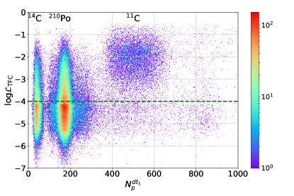
FIG. 1: Distribution of log($\mathcal{L}_{\rm{TFC}}$) as a function of the $N_{p}^{dt_{1}}$ energy estimator. The plot is built using the entire set of data surviving the selection cuts described in Sec. II. The regions dominated by the abundant internal background of ¹⁴C and ²¹⁰Po are indicated by the corresponding labels. The green-dashed horizontal line represents the $\mathcal{L}_{\rm{TFC}}$-threshold, above/below which the events are assigned to the TFC-tagged/subtracted energy spectrum. It is clearly visible that the majority of the events of the ¹¹C energy decay spectrum lies above this threshold.

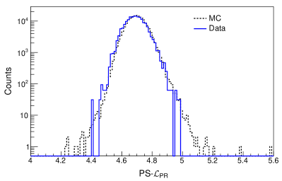
FIG. 2: Comparison of the distributions of the PS-$\mathcal{L}_{\rm{PR}}$ parameter for ²¹⁴Bi events extracted from data (blue, continuous line) and generated using MC (black, dashed line). The MC sample of ²¹⁴Bi was generated using the same spatial distribution of the ²¹⁴Bi events of the data. The simulation also takes into account the proper values of the working channels $N^{\prime}(t)$.

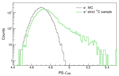
FIG. 3: Comparison of the distributions of the PS-$\mathcal{L}_{\rm{PR}}$ variable for MC generated $e^{-}$ events (black, dashed line) and for $e^{+}$ events selected from the data (green, continuous line). The latter events are a high-purity ¹¹C sample, obtained with the optimized TFC method, using very strict cuts on the energy and on the time correlation with the neutron and muon tracks.

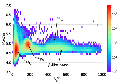
FIG. 4: Distribution of PS-$\mathcal{L}_{\rm{PR}}$ pulse-shape discriminator as a function of $N_{p}^{dt_{1}}$ energy estimator. The plot is built using the entire set of data surviving the selection cuts described in Sec. II. The comparison with Fig. 3 allows to identify the range of values belonging to the $\beta^{-}-$like band indicated by the arrow.

III.1 Pulse shape discrimination of $\beta^{+}/\beta^{-}$events

The residual amount of ¹¹C in the TFC-subtracted spectrum can be disentangled from the neutrino signal through variables with $\beta^{+}/\beta^{-}$ pulse-shape discrimination capability Bellini et al. (2012, 2014b). We build these variables considering that the Probability Density Function (PDF) of the time detection of the scintillation light is different for $\beta^{+}$ and $\beta^{-}$ events for two reasons: ${\it i)}$ for $\beta^{+}$ events, in 50% of the cases, the $e^{+}$ annihilation is delayed by ortho-positronium formation, which survives in the liquid scintillator with a mean time $\tau$ $\sim$ 3 ns Franco et al. (2011); ${\it ii)}$ the topology $e^{+}$ energy deposit is not point-like, due to the two back-to-back 511 keV annihilation $\gamma$s. These two features originate a pattern of the energy deposit of $\beta^{+}$ with a larger time and spatial spread than the corresponding one generated by $\beta^{-}$. Based on this fact, a pulse–shape (PS) discrimination algorithm has been constructed using the neural network of a Boosted Decision Tree (BDT) and used for previous analysis as detailed in Bellini et al. (2014b). In the present analysis, we have introduced a novel discrimination parameter, called PS-$\mathcal{L}_{\rm{PR}}$, defined as the maximum value of the likelihood function $\mathcal{L}_{\rm{PR}}$ used in the position reconstruction (PR), divided by the value of the energy estimator. The latter normalisation removes the $\mathcal{L}_{\rm{PR}}$ energy-dependence, since it is calculated as the summation over the collected hits Bellini et al. (2014b). The PR-algorithm is based on the expected distribution of the arrival times of optical photons on the PMTs. For all events, the algorithm uses the scintillation light emission PDF of point-like $\beta^{-}$ events. For this reason the distribution of the maximum likelihood value shows some discrimination capability for different types of particles, if they originate photon time patterns distinct from that of $\beta^{-}$.

The study of the performances of the PS-L_PR variable demands, from one side, the identification of samples of true $\beta^{-}$ and $\beta^{+}$ events and, from another side, it requires to properly account for the variable number of working channels that influences its value.

A pure, high-statistics $\beta^{-}$ sample can only be obtained from a limited time period of the water-extraction phase of the scintillator purification campaign. During this time, a temporary ²²²Rn contamination entered the detector. Using the space-and-time correlation of the fast coinciding ²¹⁴Bi($\beta^{-}$)-²¹⁴Po ($\alpha$) decays, we have tagged about $10^{4}$ ²¹⁴Bi events. The ability of the MC to reproduce the PS-L_PR parameter of these events and the comparison to data is shown in Fig. 2. The agreement between data and simulation demonstrates that the MC can accurately construct the PDF of this parameter for the entire set of data thus accounting for the variable number of working channels.

Our best $\beta^{+}$ sample is obtained from the TFC tagged events with hard cuts on the energy and on the time correlation with the neutron and muon tracks. These events are selected from the whole data set and thus they naturally follow the live-channels distribution. The discrimination capability of PS-L_PR is demonstrated comparing them with a MC sample of pure electrons with a flat energy distribution in the energy interval of the ¹¹C events, while also following the realistic live channel distribution over the whole data set. The PS-L_PR for these MC generated electrons was used as $\beta^{-}$ sample in a further analysis (analytical multivariate fit) described in Sec. IV). Figure 3 shows the distribution of the PS-L_PR parameter for the MC generated electrons compared with that of $\beta^{+}$ events obtained from ¹¹C data. The difference between the two distributions at high values of PS-$\mathcal{L}_{\rm{PR}}$ is the key element allowing the discrimination between $\beta^{-}$ and $\beta^{+}$. Note that we do not need to build a position reconstruction algorithm based on the time profile of the scintillation light of $\beta^{+}$ events. Figure 4 shows the PS-$\mathcal{L}_{\rm{PR}}$ pulse-shape discriminator as a function of $N_{p}^{dt_{1}}$ energy estimator for events selected with the cuts described in Sec. II and used in the present analysis.

It is interesting to note that the comparison between the BDT and PS-$\mathcal{L}_{\rm{PR}}$ parameters, using the samples of true $\beta^{-}$ and $\beta^{+}$ events, shows that they have similar discrimination power and they similarly help in reducing the systematic uncertainty of the $pep$ $\nu$s result. However, the use of PS-$\mathcal{L}_{\rm{PR}}$ offers some advantages like its simplicity, the fact that it can be calculated without the training procedure necessary for BDT (that suffers the limited size of the available $\beta^{-}$ training sample), and finally, the possibility to easily reproduce it through the MC.

IV Multivariate fit

The most powerful signatures for the detection of solar neutrinos in Borexino are the shapes of the energy spectra from electrons that underwent elastic scattering interactions with neutrinos. However, the recognition of these shapes is somewhat obstacled by the contribution of various types of background events. In addition, the spectral details are also masked through the finite energy resolution of the detector and eventually distorted by non-linear effects linking the energy deposit in the scintillator and the observed energy estimator.

Signal and background can be disentangled through an accurate fit. In order to enhance our sensitivity to the neutrino signal, we have adopted in the entire LER the multivariate fit approach already exploited in Bellini et al. (2012). We maximize a binned likelihood function containing the information from the TFC-tagged and TFC-subtracted energy spectra. Additional information from the PS-$\mathcal{L}_{\rm{PR}}$ parameter and the radial distributions of the events in the optimized energy regions are included in the fit. The radial information is important to accurately measure the background rates due to external $\gamma$s produced by the contamination of the PMTs and the supporting SSS. The pulse shape parameter PS-$\mathcal{L}_{\rm{PR}}$ helps in the separation of the residual ¹¹C($e^{+}$) background from the $e^{-}$–like components, and this is relevant for the determination of $R_{pep}$ and $R_{\mathrm{CNO}}$.

Several ingredients are necessary to perform the fit. The first one is a background model, that is a list of possible radioactive contaminants that we assume give a contribution to the measured signal. The second one is the detector response function, i.e. a full model of the distributions of all the physical variables that we measure. The knowledge of the detector response function allows the prediction of the probability density functions of all the quantities entering the fit procedure.

As done in previous Borexino analyses, we have adopted two complementary methods to build the detector response function: an analytical approach and a MC based procedure. The only free parameters of the fit in the MC approach are the interaction rates of neutrino and background species, while in the analytical method (see later), in addition, some of the parameters related to the response function and to the energy scale are also free and determined by the fit procedure. These two methods share the same background model.

Fitting tools based on the use of Graphical Processing Units (GPU) have been developed and used with the analytical fit method. They decrease the computation time by about 3 orders of magnitude compared with the standard CPU based algorithms previously used Ding et al. (2018).

IV.1 Multivariate Likelihood Function

The TFC-subtracted and TFC-tagged data-sets are fitted simultaneously by maximising a likelihood function $\mathcal{L}_{3D}(\vec{\theta}|\vec{k})$ defined as

$$\mathcal{L}_{3D}(\vec{k}|\vec{\theta})=\mathcal{L}^{TFC}_{sub}(\vec{k}|\vec{\theta})\cdot\mathcal{L}^{TFC}_{tag}(\vec{k}|\vec{\theta}).$$ (1)

The symbol $\vec{\theta}$ indicates the set of the arguments with respect to which the function is maximised and $\vec{k}$ generically indicates the set of the experimental data used to evaluate the likelihood. The two factors in Eq. 1 are the likelihood functions related to TFC-subtracted and TFC-tagged energy spectra, respectively.

$\mathcal{L}^{TFC}_{sub}(\vec{k}|\vec{\theta})$ is the standard Poisson binned likelihood function:

$$\mathcal{L}^{TFC}_{sub}(\vec{k}|\vec{\theta})=\prod_{j,l,m=0}^{N_{E,R,P}}\frac{\lambda_{jlm}^{k_{jlm}}(\vec{\theta})}{k_{jlm}!}e^{-\lambda_{jlm}(\vec{\theta})},$$ (2)

where $\vec{k}$ in this case is the ensemble of the data entries $k_{j,l,m}$ in the energy bin $j$, position bin $l$, and pulse shape parameter bin $m$; $\lambda_{j,l,m}(\vec{\theta})$ are the expected number of entries in the same bins, and $N_{E,R,P}$ are the total number of energy, radial, and pulse shape parameter bins. $\mathcal{L}^{TFC}_{tag}(\vec{k}|\vec{\theta})$ is constructed in a similar way but it does not include the pulse shape variable:

$$\mathcal{L}^{TFC}_{tag}(\vec{k}|\vec{\theta})=\prod_{j,l=0}^{N_{E,R}}\frac{\lambda_{j,l}^{k_{j,l}}(\vec{\theta})}{k_{j,l}!}e^{-\lambda_{j,l}(\vec{\theta})}.$$ (3)

and $\vec{k}$ represents in this case the set of data entries $k_{j,l}$ in the energy and radial bins $j,l$ integrated with respect to the pulse shape parameter. The signal of ¹¹C in the TFC-tagged spectrum is relatively strong compared to the other spectral components and the fit procedure extracts it very efficiently thanks to its spectral shape. This is the reason driving the choice of using the two dimensional (2D) likelihood function of Eq. 3 for the TFC-tagged spectrum instead of a complete function of Eq. 2 that, for the TFC-tagged spectrum, only increases the computation time without bringing additional information.

Both the TFC-subtracted and TFC-tagged spectra are fitted keeping the rates of the majority of the components in common, except ¹¹C itself, ⁶He and ¹⁰C (which have cosmogenic origin), and ²¹⁰Po, that is not distributed homogeneoulsy through the detector volume.

Constraints on the values of the multivariate fit parameters are implemented (if not specified otherwise) as multiplicative Gaussian terms in the likelihood function.

The likelihood function of Eq. 2 and Eq. 3 are exactly the ones which are maximized using our most recent version of the MC-based fit procedure (see Sec. V.1). Precisely, we generate with the MC every signal and background component and we build and properly normalize 3D (or 2D) histograms of the simulated number of events as a function of the energy estimator, PS-$\mathcal{L}_{\rm{PR}}$ parameter, and radius (or of the energy estimator and radius only). The quantities $\lambda_{jlm}$ and $\lambda_{jl}$ of Eq. 2 and Eq. 3 represent the sum of the bin content of the histograms, each one weighted by the rate of the specific component ($\vec{\theta}$).

Earlier versions of the MC fit and the present analytical fit maximize an approximated version of the likelihood $\mathcal{L}_{3D}(\vec{k}|\vec{\theta})$, as already described in Bellini et al. (2014b). This function, called $\mathcal{L}(\vec{k}|\vec{\theta})$, is written as a product of four factors coming from the TFC-subtracted and TFC-tagged energy spectra ( $\mathcal{L}^{TFC}_{E,sub}$ and $\mathcal{L}^{TFC}_{E,tag}$) and from the PS-$\mathcal{L}_{\rm{PR}}$ ($\mathcal{L}_{P}$) and radial ($\mathcal{L}_{R}$) distributions of events in the ¹¹C-energy-range of the TFC-subtracted spectrum:

$$\mathcal{L}(\vec{k}|\vec{\theta})=\mathcal{L}^{TFC}_{E,sub}(\vec{k}|\vec{\theta})\cdot\mathcal{L}^{TFC}_{E,tag}(\vec{k}|\vec{\theta})\cdot\mathcal{L}_{P}(\vec{k}|\vec{\theta})\cdot\mathcal{L}_{R}(\vec{k}|\vec{\theta}).$$ (4)

The first two terms, $\mathcal{L}^{TFC}_{E,sub}(\vec{k}|\vec{\theta})$ and $\mathcal{L}^{TFC}_{E,tag}(\vec{k}|\vec{\theta})$, are Poisson likelihoods (like Eq. 2 and  3) with $\vec{k}$ being the data entries $k_{j}$ in the energy bin $j$ integrated with respect to the other variables.

The other two terms in Eq. 4 have been built considering that in the framework of the analytical approach, there is no model able to produce precise multi–dimensional PDFs. Thus we have projected the events, from the optimized energy intervals of the TFC-subtracted spectrum and integrated over energy ranges larger than the binning of the energy spectrum, into 1D histograms of the pulse-shape and radial distributions. $\mathcal{L}_{P}(\vec{k}|\vec{\theta})$ and $\mathcal{L}_{R}(\vec{k}|\vec{\theta})$ of Eq. 4 are then built fitting these 1D distributions using PDFs obtained either from the data (high purity ¹¹C sample for $\beta^{+}$ pulse shape) or based on the MC simulation ($\beta^{-}$ pulse shape, radial distributions). In the calculation of the corresponding likelihoods, we introduce a correlation between the number of counts in different histograms, as events that are in the energy spectrum will also be entries in the projections. To handle this issue, we normalise the functions to the total number of entries $N$ in the projected data histograms. Consequently, we define the likelihood of the PS-$\mathcal{L}_{\rm{PR}}$ parameter as we did in Bellini et al. (2014b) for the previously used PS-BDT parameter:

$$\mathcal{L}_{P}(\vec{k}|\vec{\theta})=\prod^{N_{P}^{1D}}_{m=1}\frac{a\lambda_{m}^{k_{m}}(\vec{\theta})e^{-a\lambda_{m}(\vec{\theta})}}{k_{m}!},$$ (5)

where the scaling parameter $a$ enforces the normalisation and is set such

$$N=a\sum^{N_{P}^{1D}}_{m=1}\lambda_{m}(\vec{\theta}),$$ (6)

where $N$ is the total number of entries in the projected histogram and $a$ is a scaling factor. Here, $k_{m}$ is the actual number of entries of bin $m$ of the 1D projection of the PS-$\mathcal{L}_{\rm{PR}}$ distribution in a fixed energy interval, $N_{P}^{1D}$ is the total number of bins of this histogram, and $\lambda_{m}(\vec{\theta})$ represents the expected content in bin $m$. $\mathcal{L}_{R}(\vec{k}|\vec{\theta})$ is defined in a way similar to $\mathcal{L}_{P}(\vec{k}|\vec{\theta})$.

The results of the MC-based fit, which is either performed using $\mathcal{L}_{3D}(\vec{k}|\vec{\theta})$ or $\mathcal{L}(\vec{k}|\vec{\theta})$, are consistent, confirming that no systematic uncertainty is introduced when using the approximated likelihood function.

V Detector response function

V.1 The Monte Carlo method

The MC code developed for Borexino Agostini et al. (2018b) is a customised Geant4-based simulation package Agostinelli et al. (2003), which can simulate all processes following the interaction of a particle in the detector (energy loss including ionisation quenching in the scintillator; scintillation and Cherenkov light production; optical photon propagation and interaction in the scintillator modelling absorption and re-emission, Rayleigh scattering, interaction of the optical photons with the surface of the materials; photon detection on the PMTs, and response of the electronics chain) including all known characteristics of the apparatus (geometry, properties of the materials, variable number of the working channels over the duration of the experiment as in the real data) and their evolution in time. The code thus produces a fully simulated detector response function because it provides a simulated version of all the measured physical variables.

All the MC input parameters have been chosen or optimised using samples of data independent from the ones used in the present analysis (laboratory measurements and Borexino calibrations with radioactive sources Back et al. (2012)) and the simulation of the variables relevant for the present analysis has reached sub-percent precision Agostini et al. (2018b).

Once the MC input parameters have been tuned, the PDFs of all the needed variables related to each of the $\nu$ and background components are built simulating events according to the specific energy spectrum. In order to properly reproduce the spatial dependence of the energy response, events are simulated in the detector following their expected spatial distribution: while the $\nu$ and most of background events are expected to be uniformly distributed in the detector, ²¹⁰Po decays are simulated according to their actual spatial and time distribution obtained from experimental data. Note that data events due to the $\alpha$ decay of ²¹⁰Po are efficiently identified by tagging ²¹⁰Po with a pulse–shape discrimination method based on Multilayer Perceptron (MLP) algorithm Agostini et al. (2017b) (a particular class of neural network algorithms). Similarly, $\gamma$s from external background are generated on the SSS and PMTs surfaces so that the radial distribution of the interactions inside the scintillator volume shows a clear decrease from the outer region of the detector towards the center.

Events generated according to the theoretical signal and background energy spectra are then processed as real data. As already anticipated, for every species, 3D or 2D histograms are built for the energy estimators, the reconstructed radius, and the PS-$\mathcal{L}_{\rm{PR}}$ variable. When properly binned and normalized, these histograms represent the PDFs to be used in the fit and they provide the values $\lambda_{jlm}(\vec{\theta})$ in Eq. 2 and $\lambda_{jl}(\vec{\theta})$ in Eq. 3. In the MC approach there are no free fit parameters other than the interaction rates of all species. The goodness of the fit simultaneously demonstrates the accuracy of the MC simulation, as well as the stability of the detector response over the period of five years.

In the wide energy range covered by this analysis, there is a huge difference between the number of measured counts per bin in the lower and in the higher energy regions. In the construction of the 3D PDFs, the need to simulate large numbers of events becomes really important, since they are scattered over a larger number of bins. To mitigate the consequences due to low populated bins and to have a good approximation to a $\chi^{2}$, we have replaced the energy estimator and the radius $R$ with some transformed variables. We choose to use $R^{3}$ instead of $R$, thus using bins of 5 m³ each and still achieving a very effective separation of the external background from the bulk components. Similarly, we introduced a transformed variable $N_{h^{\prime}}$ based on the $N_{h}$ energy estimator: this change of variable is equivalent to adopting a variable binning size that scales with energy proportionally to the width of the $N_{h}$ distribution obtained simulating mono-energetic electrons. This approach allows to reduce the statistical fluctuations without losing any physical information. As a by-product, this efficient binning significantly reduced the computing time needed to perform a single fit, speeding up the analysis of the MC pseudo–experiments used to estimate the statistical and systematic uncertainties of the measurement described in Section VI.

The multivariate analysis was not applied on the whole energy range: the radial information was considered only for $N_{h}>290$ to exclude from the analysis the spatial distribution of ²¹⁰Po, while the PS-$\mathcal{L}_{\rm{PR}}$ was used where ¹¹C is present ($409<N_{h}<645$). The shape of the probability density function of the PS-$\mathcal{L}_{\rm{PR}}$ variable for $\beta^{+}$ was obtained from an empirical parametrisation of the distribution generated by the MC, with an additional small shift to compensate differences between the MC simulation outcome and a sample of strictly selected ¹¹C events.

Parameter	Fix./Free	Meaning/Approach to fixing	Value
$Y^{pe}_{0}$	free	Photoelectron yield [p.e./MeV] for events in the detector center and with $N_{tot}$=2000 PMTs	551 $\pm$ 1
$g_{C}$	fixed	Fit $N_{p}^{dt_{1(2)}}$ vs true $N_{pe}$ of MC with Eq. 14 using MC mono-energetic electron samples at 4 energies, simulated along the whole data-set.	0.101
$p_{t}$	fixed	Fraction of a single photoelectron charge spectrum below the electronics threshold; fixed from the earlier calibration measurements and calculations.	0.12
$f_{Ch}$	fixed	Relative weight of the scintillation and Cherenkov light; fixed by performing many analytical fits on data with it as a free/fixed parameter.	1.0
$F_{Ch}(E)$	fixed	$$F_{Ch}(E)=(C_{0}+C_{1}\cdot x+C_{2}\cdot x^{2}+C_{3}\cdot x^{3})(1+C_{4}\cdot E)$$ (7) $x=\ln{(1+E/E_{0})}$; $E_{0}$ = 0.165 MeV	$C_{0}=1.415$; $C_{1}=-3.397$; $C_{2}=1.107$; $C_{3}=0.072$; $C_{4}=1.337$
$Q(E)$	fixed	Quenching term summarising the effects related to non-linearity of the scintillator response according to Birk’s quenching model Bellini et al. (2014b): $$Q(E,k_{B})=\frac{1}{E}\int_{0}^{E}\frac{dE^{\prime}}{1+k_{B}dE^{\prime}/dx},$$ (8) where $k_{B}$ is the Birk’s constant, and Q(E) can be parametrised as: $$Q(E,k_{B})=\frac{A_{1}+A_{2}\ln E+A_{3}\ln E^{2}}{1+A_{4}\ln E+A_{5}\ln E^{2}};$$ (9) fixed from the fit of $N_{pe}$ vs $E$ with MC simulation of $\gamma$ calibration data.	$k_{B}[\rm{cm/MeV}]=0.0109$; $A_{1}=0.972$; $A_{2}=0.201$; $A_{3}=0.0105$; $A_{4}=0.195$; $A_{5}=0.014$
$v_{1}$	fixed	Relative variance of the probability that a PMT triggers for events uniformly distributed in the detector volume, calculated using dedicated MC studies. It has some energy dependence and then we are using a value averaged over the LER.	0.16
$v_{T}^{0}$	free	Spatial non-uniformity of the number of triggered PMTs.	0.50 $\pm$ 0.37
$v_{N}$	free	Scintillator intrinsic resolution parameter for $\beta$s (caused by $\delta$-electrons) that also effectively takes into account other contributions at low energies.	11.5 $\pm$ 1.0
$v^{q}_{T}$	fixed	Non-uniformity of the light collection, calculated from MC events uniformly distributed in FV.	7.0
$v_{T}^{\alpha}$	free	Spatial non-uniformity resolution, corresponding to the width of 210Po-$\alpha$ peak.	4.73 $\pm$ 0.21
$\sigma_{d}$	fixed	PMT dark noise contribution	0.23 $N^{dt_{1}}_{p}$, 0.4 $N^{dt_{2}}_{p}$

TABLE 1: Summary of the parameters used in the analytical model of the energy response function. In case of the free parameters, the values given in the table are obtained with the multivariate analytical fit of the data discussed in this paper and reported in section VII. Only statistical errors are shown here. Energy is expressed in MeV; $v_{T}^{0}$, $v_{T}^{\alpha}$ ($v_{T}^{q}$) must be multiplied by $10^{-6}$ ($10^{-4}$).

V.2 The analytical model of the energy response function

In the analytical approach, we introduce a PDF for the energy estimator under consideration and analytical expressions for its mean value and variance. This PDF describes the detector’s energy response function to mono–energetic events and, in brief, it is mainly influenced by the number of scintillation and Cherenkov photons and effects due to the non–uniformity of the light collection. As already anticipated, we then transform the energy spectra of each species into the corresponding distributions of the energy estimators. Effects like the ionisation quenching in the scintillator, the contribution of the Cherenkov light, the spatial dependence of the reconstructed energy and its resolution are accounted for through some parameters, part of which are fixed, while others are free to vary in the final fit.

We describe here the present model for $N_{p}$ which is derived from Bellini et al. (2014b), with several improvements to extend the energy range of the fit to the entire LER. The same model describes the variables $N_{p}^{dt_{1(2)}}$. All used energy estimators are obtained after normalising the corresponding measured values to a reference configuration of $N_{tot}=2000$ channels (defined in Sec. II).

As energy response function for the entire LER, we use the scaled Poisson function $f(N_{p})$ (and similarly $f(N_{p}^{dt_{1(2)}})$) already introduced for analyzing events in the lowest region of the energy spectrum and detailed in Agostini et al. (2015) and in Smirnov et al. (2016)

$$f(N_{p})=\frac{m^{(N_{p}s)}}{(N_{p}s)!}\exp^{-m}$$ (10)

The two free parameters of this function, $m$ and $s$, are fixed using the expressions for the mean value $\bar{N}_{p}(E)$ and variance $\sigma_{p}^{2}$ developed in the context of our model and described below:

$$m=\frac{\bar{N}_{p}^{2}(E)}{\sigma_{p}^{2}}$$ (11)

and

$$s=\frac{\sigma_{p}^{2}}{\bar{N}_{p}(E)}$$ (12)

In order to obtain $\bar{N}_{p}(E)$ we first consider that the mean number of photoelectrons $\bar{N}_{pe}(E)$ for each event of energy $E$ takes its main contribution from the scintillation photons with a sub-dominant correction from the Cherenkov light, and it can be written as follows

$$\bar{N}_{pe}(E)=Y^{pe}_{0}\cdot[Q(E)\cdot E+f_{Ch}\cdot F_{Ch}(E)]$$ (13)

where $Y^{pe}_{0}$ is the photoelectron yield expressed in photoelectrons/MeV for events in the detector center; the quenching term, $Q(E)$, accounts for non-linearity of the scintillator response; $F_{Ch}(E)$, an analytical parametrisation of Cherenkov light dependence on energy valid for electrons, provides the smooth transition between linear dependency at the energies above 1–2 MeV and zero contribution for electrons below the Cherenkov threshold $E_{0}$ = 0.165 MeV; $f_{Ch}$ is a parameter allowing to adjust the relative weight of the scintillation and Cherenkov light. Table 1 reports details of the analytical expressions.

Similarly to that described in Bellini et al. (2014b), $\bar{N}_{p}(E)$, is linked to $\bar{N}_{pe}(E)$ through

$$\bar{N}_{p}(E)=N_{tot}\left[1-e^{-\mu}\left(1+p_{t}\mu\right)\right]\left(1-g_{C}\mu\right)$$ (14)

where $\mu=\dfrac{\bar{N}_{pe}(E)}{N_{tot}}$, $g_{C}$ is a geometric correction factor, calculated for the given fiducial volume, and $p_{t}$ is the fraction of a single photoelectron signal below the electronics threshold. These expressions extend the ones previously used in Bellini et al. (2014b) with the introduction of the $f_{Ch}$ and $p_{t}$ parameters.

The second ingredient of the analytical model is the variance $\sigma^{2}_{p}$ of the $N_{p}$ energy estimator. It is described by the following expression which extends the model already described in  Bellini et al. (2014b) in particular with the modification of the term linear with $\bar{N}_{p}(E)$ and the addition of a quadratic one

$$\sigma^{2}_{p}=f_{eq}\left[1-\left(1+v_{1}\right)p_{1}\right]\bar{N}_{p}(E)+v_{T}^{0}\bar{N}_{p}^{3}(E)+$$

$$+\ v^{q}_{T}{\left(\mu\frac{p_{0}}{p_{1}}\right)}^{2}\bar{N}_{p}^{2}(E)+v_{N}\bar{N}_{p}(E)+\sigma^{2}_{d}$$ (15)

where $v_{1}$ is the relative variance of the PMT triggering probability for events uniformly distributed in the detector volume, $p_{1}=1-e^{-\mu}$ is the probability of having a signal at any PMT, $p_{0}=e^{-\mu}$ is the probability of absence of the signal, $v_{T}^{0}$ accounts for the spatial non-uniformity of the number of triggered PMTs, $v^{q}_{T}$ accounts for the non-uniformity of the light collection, $v_{N}$ is the intrinsic resolution parameter of the scintillator for $\beta$s that effectively includes other contributions at low energies, and the last term $\sigma_{d}$ describes the effects of the dark noise of the PMTs. The channel equalization factor $f_{eq}$ is the ratio between $N_{tot}$ and the actual number of working PMTs and it changes during the data taking period.

In summary, the cubic term takes into account the variance of the number of the triggered PMTs for the events with fixed collected charge in the IV. The quadratic term takes into account the variance of the light collection function over the detector, and is generally weaker compared to the cubic term (and was neglected in previous analyses with more uniform PMTs distribution).

Formula 15 was derived analytically and verified against the MC simulations. For $\alpha$ particles we are using a simplified form with only the first and cubic term of relation 15 since we need to model a single energy point (²¹⁰Po). It is thus not necessary to follow the energy dependence of the variance. The coefficient of the cubic term is called $v_{T}^{\alpha}$ and it corresponds to the width of the ²¹⁰Po-$\alpha$ peak. As anticipated, we use the previous relations also for describing the mean value and variance of the estimators $N_{p}^{dt_{1(2)}}$.

Most of the above listed parameters are tuned using data independent from the ones used in the solar neutrino fit, calibrations or MC and are fixed in the fit ($Q(E)$, $f_{Ch}$, $p_{t}$, $g_{C}$, $v_{1}$, $v_{T}^{q}$), while other parameters ($Y^{pe}$, $v_{T}^{\alpha}$, $v_{T}^{0}$, $v_{N}$) are left free to vary in the fit, together with the neutrino and background interaction rates. The two parameters $p_{t}$, $g_{C}$ could be in principle free fit parameters, however they are fixed because the fit results have a low sensitivity to them.

In summary, the model has one free parameter describing the yield and three free parameters describing the energy resolution. Leaving the above listed parameters free gives the analytical fit the freedom to account for unexpected effects or unforeseen variations of the detector response in time. Table 1 reports all the parameters, free or fixed, appearing in the analytical fit with a short explanation about how they are obtained. In case of parameters kept free in the fit, we report in the table the values obtained fitting the present data set as described in this paper. The corresponding values of the $\nu$ interaction rates and background are reported in section VII.

V.3 Handling of the energy variables in the fit

We perform the fit of the energy spectra with the experimental data binned as a function of the energy estimators instead of trasforming that distributions into the energy scale. Among the reasons driving this choice we remark that the analytical approach does not assume a priori knowledge of the precise energy transformation rules and the energy scale is automatically adjusted while fitting the experimental data. The use of the transformed experimental spectra would significantly slow down the fitting procedure, as the data reprocessing will be needed each time the energy scale parameters are changed in the fit. In addition, the presence of the contributions from ¹⁴C and ²¹⁰Po with very high statistics makes the fit sensitive to tiny details of the energy response function (response to the monoenergetic event with a fixed energy distributed uniformly in the detector’s volume). The shape of the energy response for the detected number of p.e. (or the number of the triggered PMTs) in the sub-MeV energy region is defined mainly by the statistical factor, with small additional smearing due to the non-uniformity of the amount of the collected light throughout the detector. The study performed using MC model showed that the shape of the charge response can be approximated by the generalized gamma function, and the shape of the $N_{p}$ response can be approximated by the scaled Poisson function. But the energy response function in the energy scale does not allow a simple description with an analytical function, and thus complex calculations would be necessary if the transformed energy is used. In the MC approach the transformation to the energy scale is in principle feasible, because the energy scale and energy response in this approach are fixed from the calibrations, but it was not applied to keep internal consistency with the analytical approach.

Moreover, the amount of light emitted for a given energy deposit in the scintillator differs for the electrons, $\gamma$s and $\alpha$ particles and then the energy scale calibrated for electrons is not valid for $\alpha$s and $\gamma$s. The experimental spectrum contains contributions from all these types of particle and the event-by-event identification of the type of interaction is not possible while the different contributions are statistically identified using the fit procedure. The binning of the data in the physical energy scale (as shown in the figures reporting the fit results) is performed only after the fit is completed.

VI Sensitivity studies

Sensitivity studies have been performed by generating many pseudo-experiments with the MC and fitting this simulated data using the same response functions adopted for fitting the real experimental data, using both analytical and MC procedures. The simulated data of the pseudo-experiments are obtained from a random sampling of PDFs produced with the full Borexino MC, including solar neutrino interaction rates as predicted by the HZ/LZ–SSM and with the rates of the different background components compatible with the final results presented in this work. As an example, Fig. 5 shows the distribution of the results of the MC fit of 6700 pseudo-experiments each one with the same exposure as the real data. In this particular example, by construction, the fit model perfectly matches the simulated data. The 1D distributions of the fit results, i.e. the rates $R$ of different solar neutrino and background species, are Gaussian and do not show any significant biases with respect to the rates used as simulation inputs. The widths of these distributions show the expected statistical precision of the measurement of the corresponding component. The shapes of the analogous 2D distributions visualize the correlations among the different components. In particular, we underline that since the energy spectrum of the CNO neutrinos is quite similar to that of the ²¹⁰Bi internal contamination and the fit procedure cannot disentangle them, the sensitivity studies for all the $pp$-cycle neutrino and background components are performed by constraining the CNO rate. These results are depicted in the left portion of Fig. 5 with $R_{\rm CNO}$ generated and constrained assuming, as an example, the HZ–SSM. The same constraint on $R_{\rm CNO}$ is used in fitting the real data, as it will be reported below. Some additional significant correlations are present among some of the various species, as the figure is showing. This is one of the reasons why the best accuracy in the determination of the interaction rates of solar neutrinos is obtained by fitting the entire energy spectrum, as in the present analysis, thus best using all the available information about details of the entire spectral shapes, instead of choosing partial energy regions.

The top right inset in Fig. 5 demonstrates the sensitivity of the present data set to CNO neutrinos. In this case, no constraint on $R_{\rm CNO}$ is applied, but, to decrease the effect of the degeneracy of the spectral shapes, a constraint on the ratio between $R_{pp}$ and $R_{pep}$, as expected from the SSM, is applied. It is interesting to note the strong anti-correlation between the ²¹⁰Bi and CNO components which is originated by the above discussed similarities of their energy spectra.

Finally, Fig. 6 is obtained removing all the constraints on the CNO and $pep$ components and clearly shows that the strong correlations (and anti-correlations) among $R_{\rm CNO}$, $R_{pep}$, and the ²¹⁰Bi decay rate significantly limit the possibility to determine all the three species at the same time.

Similar MC studies have been performed to quantify the systematic uncertainty associated to the fit models, by generating MC data with a response function modified with respect to the one used in the fit (see next section). Finally, pseudo-experiments MC data have been used to obtain the distribution of the likelihood functions and thus evaluate the p-values of our results.

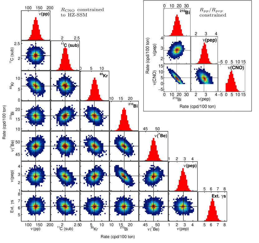
FIG. 5: The figure shows the distributions of the interaction rates (cpd/100 ton) of solar $\nu$ and of the background species as they result from the MC fit of pseudo-experiments simulated with the same exposure as the experimental data discussed in this paper. The fit is performed in the entire LER region and, as in the real data analysis, penalty terms are added in the likelihood to constrain the values of the ¹⁴C and pileup rates within the measured ones. It is interesting to note the correlation between the $pp$ and ⁸⁵Kr rates, physically driven by the fact that a not negligible portion of the ⁸⁵Kr spectrum lies in the energy region around about 200 keV where we are sensitive to the $pp$ $\nu$s signal. In the left plot, 6700 pseudo-experiments have been generated assuming the $R_{\rm CNO}$ according to HZ-SSM and fitted imposing a constraint on $R_{\rm CNO}$ to the same value. The same MC PDFs have been used to simulate and fit data, so these plots show only uncertainties due to statistical fluctuations and the effects of the correlations among the various components. The top right inset represents the results of the fit of 10000 pseudo-experiments fitted with the MC method while keeping the $R_{\rm CNO}$ free but constraining the $R_{pp}/R_{pep}$ ratio to (47.7 $\pm$ 0.8) (HZ-SSM Vinyoles et al. (2017), Esteban et al. (2017)). Constraining $R_{pp}$/$R_{pep}$ to the LZ-SSM prediction, 47.5 $\pm$ 0.8, gives consistent results. The study included all the background and neutrino species: here we only show those components that mostly influence the sensitivity to CNO neutrinos.

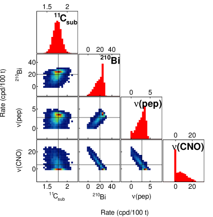
FIG. 6: This figure shows the results of the fit of MC simulated experiments obtained in the same conditions of Fig. 5 but, this time, removing all the constraints on $R_{\rm CNO}$ and $R_{pep}$. We only show here the correlation between $pep$, CNO, ¹¹C and ²¹⁰Bi, but the study included all the spectral components. The significant correlations among these species forbid to measure at the same time $R_{\rm CNO}$ and $R_{pep}$ and to determine the ²¹⁰Bi decay rate. As described in the text, we have constrained the CNO rate to get the $pep$ one and set a constraint on the ratio $R_{pp}$/$R_{pep}$ to obtain a limit on the CNO flux.

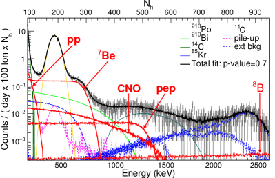
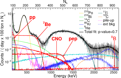
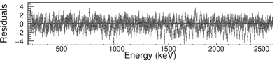
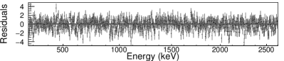
FIG. 7: Multivariate fit results (an example obtained with the MC method) for the TFC-subtracted (left) and the TFC-tagged (right) energy spectra, with residuals. The sum of the individual components from the fit (black lines) is superimposed on the data (grey points). The analysis has been performed using $N_{h}$ as energy estimator and the transformation to keV-energy scale was perfomed only for the plotting purposes. The residuals are calculated in every bin as the difference between the data counts and the fit result, divided by the square root of the data counts.

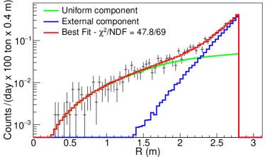
FIG. 8: An example of the multivariate fit showing the radial (top) and the PS-$\mathcal{L}_{\rm{PR}}$ (bottom) distributions of the events (black crosses) from the TFC-subtracted spectrum, in the energy intervals $N_{h}>290$ and $409<N_{h}<645$, respectively.

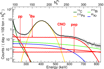
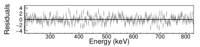
FIG. 9: Results of the fit for TFC-subtracted energy spectrum zoomed in to the lowest energy region (an example obtained with the analytical method) and residuals. The residual are calculated as in Fig. 7.

Solar $\nu$	Borexino experimental results		B16(GS98)-HZ		B16(AGSS09)-LZ
	Rate	Flux	Rate	Flux	Rate	Flux
	[cpd/100 ton]	$\rm{[cm^{-2}s^{-1}]}$	[cpd/100 ton]	$\rm{[cm^{-2}s^{-1}]}$	[cpd/100 ton]	$\rm{[cm^{-2}s^{-1}]}$
$pp$	$134\pm 10\;^{+6}_{-10}$	$(6.1\pm 0.5\;^{+0.3}_{-0.5})\times 10^{10}$	$131.1\pm 1.4$	$5.98\,(1\pm 0.006)\times 10^{10}$	$132.2\pm 1.4$	$6.03\,(1\pm 0.005)\times 10^{10}$
$\rm{{}^{7}Be}$	$48.3\pm 1.1\;^{+0.4}_{-0.7}$	$(4.99\pm 0.11\;^{+0.06}_{-0.08})\times 10^{9}$	$47.9\pm 2.8$	$4.93\,(1\pm 0.06)\times 10^{9}$	$43.7\pm 2.5$	$4.50\,(1\pm 0.06)\times 10^{9}$
$pep$ (HZ)	$2.43\pm 0.36\;^{+0.15}_{-0.22}$	$(1.27\pm 0.19\;^{+0.08}_{-0.12})\times 10^{8}$	$2.74\pm 0.04$	$1.44\,(1\pm 0.009)\times 10^{8}$	$2.78\pm 0.04$	$1.46\,(1\pm 0.009)\times 10^{8}$
$pep$ (LZ)	$2.65\pm 0.36\;^{+0.15}_{-0.24}$	$(1.39\pm 0.19\;^{+0.08}_{-0.13})\times 10^{8}$	$2.74\pm 0.04$	$1.44\,(1\pm 0.009)\times 10^{8}$	$2.78\pm 0.04$	$1.46\,(1\pm 0.009)\times 10^{8}$
$\rm{CNO}$	$<8.1\;(95\%\,\rm{C.L.})$	$<7.9\times 10^{8}\;(95\%\,\rm{C.L.})$	$4.92\pm 0.55$	$4.88\,(1\pm 0.11)\times 10^{8}$	$3.52\pm 0.37$	$3.51\,(1\pm 0.10)\times 10^{8}$

TABLE 2: Borexino Phase-II results on $pp$, ⁷Be (862 +384 keV), $pep$, and CNO solar $\nu$s: interaction rates and fluxes inferred assuming the MSW-LMA oscillation parameters Esteban et al. (2017). The first error is the statistical derived by profiling the likelihood under Wilks’ approximation. The interval extracted is consistent with the expectation from the MC sensitivity study. The second error is the systematic uncertainty. Different contributions to the systematic error are detailed in Table 4. The result on $pep$ $\nu$s depends on whether we assume HZ-SSM or LZ-SSM metallicity for CNO $\nu$s. The remaining columns show the theoretical interaction rates and fluxes predicted by the Standard Solar Model under the high and low metallicity assumptions Vinyoles et al. (2017).

Background		Rate
		[cpd/100  ton]
14C [Bq/100 t]		$\leavevmode\nobreak\ 40.0\pm 2.0$
85Kr		$\leavevmode\nobreak\ \leavevmode\nobreak\ 6.8\pm 1.8$
210Bi		$\leavevmode\nobreak\ 17.5\pm 1.9$
11C		$\leavevmode\nobreak\ 26.8\pm 0.2$
210Po		$260.0\pm 3.0$
Ext. 40K		$\leavevmode\nobreak\ \leavevmode\nobreak\ 1.0\pm 0.6$
Ext. 214Bi		$\leavevmode\nobreak\ \leavevmode\nobreak\ 1.9\pm 0.3$
Ext. 208Tl		$\leavevmode\nobreak\ \leavevmode\nobreak\ 3.3\pm 0.1$

TABLE 3: Best estimates for the total rates of the background species included in the fit with statistical and systematic uncertainties added in quadrature. These numbers are obtained by averaging the results of the fits with the HZ and LZ hypothesis.

	$pp$		7Be		$pep$
Source of uncertainty	$-\%$	$+\%$	$-\%$	$+\%$	$-\%$	$+\%$
Fit method (analytical/MC)	-1.2	1.2	-0.2	0.2	-4.0	4.0
Choice of energy estimator	-2.5	2.5	-0.1	0.1	-2.4	2.4
Pile-up modeling	-2.5	0.5	0	0	0	0
Fit range and binning	-3.0	3.0	-0.1	0.1	1.0	1.0
Fit models (see text)	-4.5	0.5	-1.0	0.2	-6.8	2.8
Inclusion of 85Kr constraint	-2.2	2.2	0	0.4	-3.2	0
Live Time	-0.05	0.05	-0.05	0.05	-0.05	0.05
Scintillator density	-0.05	0.05	-0.05	0.05	-0.05	0.05
Fiducial volume	-1.1	0.6	-1.1	0.6	-1.1	0.6
Total systematics ($\%$)	-7.1	4.7	-1.5	0.8	-9.0	5.6

TABLE 4: Relevant sources of systematic uncertainty and their contributions to the measured neutrino interaction rates. More details are in the text.

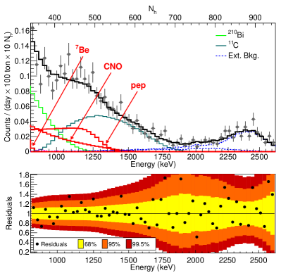
FIG. 10: TFC-subtracted energy spectrum zoomed between 800 keV and 2700 keV after applying stringent selection cuts on the radial distribution (R $\,<\,$ 2.4 m) and on the pulse-shape variable distribution (PS-$\mathcal{L}_{\rm{PR}}<\,$4.8) to better see features due to $pep$ $\nu$s interactions. The residuals (bottom plot) are the ratio between the data and the fit model.

VII Results

The interaction rates $R_{pp}$, $R_{\rm{Be}}$, $R_{pep}$ are obtained from the fit together with the decay rates of ⁸⁵Kr, ²¹⁰Po, ²¹⁰Bi, ¹¹C internal backgrounds, and the external backgrounds rates (²⁰⁸Tl, ²¹⁴Bi, and ⁴⁰K $\gamma$ rays).

In the MC approach, the MC-based pile-up spectrum Agostini et al. (2018b) is included in the fit with a constraint of (137.5 $\pm$ 2.8 cpd/100 ton) on the ¹⁴C–¹⁴C contribution based on an independent measurement of the ¹⁴C rate Bellini et al. (2014a). In the analytical approach, pile-up is taken into account with the convolution of each spectral component with the solicited-trigger spectrum Bellini et al. (2014a). Alternatively, the analytical fit uses a synthetic pile-up spectrum Bellini et al. (2014a) built directly from data. The differences between these methods are quoted in the systematic error (see Table  4).

In order to break the degeneracy between the ²¹⁰Bi and the CNO $\nu$ spectral shapes, we constrain the CNO $\nu$ interaction rate to the HZ-SSM predictions, including MSW-LMA oscillations (4.92 $\pm$ 0.56 cpd/100 ton) Vinyoles et al. (2017); Esteban et al. (2017) as anticipated in Sec. VI. The analysis is repeated constraining the CNO $\nu$ rate to the LZ-SSM predictions (3.52 $\pm$ 0.37 cpd/100 ton) and in case of difference, the two results are quoted separately. The contribution of ⁸B $\nu$s is small and its rate was constrained to the value obtained from the HER analysis Agostini et al. (2017a).

The interaction rates of solar neutrinos and the decay rates of background species, obtained by averaging the results of the analytical and MC approaches, are summarised in Tables 2 and 3, respectively.

An example of the multivariate fit (with the MC approach) is shown in Fig. 7 (TFC-subtracted and TFC-tagged energy spectra) and in Fig. 8 (radial distribution and PS-$\mathcal{L}_{\rm{PR}}$ pulse-shape distribution). The details of the fit at low energies (between $\sim$ 230 and 830 keV) can be appreciated in Fig. 9. In this example, obtained with the analytical fit procedure, the pile-up is not present as a separate fit component, since it is taken into account with the convolution method mentioned above.

To recognise the $pep$ $\nu$ contribution to the measured electron-recoil spectrum, the TFC-subtracted spectrum, zoomed into the highest energy region (between 800 and 2700 keV), is shown after applying stringent selection cuts on the radial distribution (R $<$ 2.4 m) and on the pulse-shape variable distribution (PS-$\mathcal{L}_{\rm{PR}}$ $<$4.8) (see Fig. 10): the CNO and pep neutrino interactions are clearly visible between 1250 and 1500 keV, and the spectrum is consistent with the Compton-like shoulder expected from the $pep$ line.

An extensive study of the systematic errors has been performed and the results are summarised in Table 4.

Differences between the results of the analytical and the MC fits are quoted as systematic errors. Further systematic uncertainties associated with the fitting procedure were studied by performing the fit in many different configurations by generating simulated data using a family of response functions whose parameters has been varied within calibration accuracy with respect to the nominal response function and by varying the energy estimator, the number and width of the bins, as well as the fit range).

Systematic uncertainties related to the fit models were evaluated using the method described in Sec. VI. Ensembles of pseudo-experiments were generated from a family of PDFs based on the full MC simulations and fitted using both the MC and analytical methods. PDFs including deformations due to possible inaccuracies in the modeling of the detector response (energy scale, uniformity of the energy response, shape of PS-$\mathcal{L}_{\rm{PR}}$) and uncertainties in the theoretical energy spectra (²¹⁰Bi) were considered. The magnitude of the deformation was chosen to be within the range allowed by the available calibration data.

In an additional systematic study, the fit was repeated taking into account the upper limit on the ⁸⁵Kr decay rate following the procedure described in Bellini et al. (2014b), which exploits the ⁸⁵Kr – ^85mRb delayed coincidences (⁸⁵Kr rate $<$ 7.5 cpd/100 ton at 95% C.L.).

The last three lines of Table 4 list the uncertainties associated with the determination of the exposure. The one about the fiducial volume is one of the dominant. Its value is the same as quoted in Bellini et al. (2011a) and it is estimated using calibration sources of known positions.

Fully consistent results are obtained when adopting a larger fiducial volume (R$\,<\,$3.02 m, $\lvert z\rvert$ $<$ 1.67 m). This FV contains more external background (critical for the $pep$ $\nu$s) which is, however, properly disentangled by the multivariate fit thanks to its energy shape and radial distribution. The previously published Borexino results regarding $pp$ $\nu$s Bellini et al. (2014a) and ⁷Be $\nu$s Bellini et al. (2011a) were obtained in this enlarged fiducial volume.

Finally, the analytical fit performed on a restricted energy range (not sensitive to $pp$ neutrinos) using the $N_{pe}$ energy estimator gives consistent results (within 2 $\sigma$) for $R_{\rm{Be}}$ and $R_{pep}$.

The ⁷Be solar $\nu$ flux listed in Table 2 is the sum of the two mono-energetic lines at 384 and 862 keV. It corresponds to a rate for the 862 keV line of 46.3 $\pm$ 1.1${}^{+0.4}_{-0.7}$ cpd/100 ton, fully compatible with the Borexino Phase-I measurement Bellini et al. (2011a). The ⁷Be solar $\nu$ flux is determined with a total uncertainty of 2.7 $\%$, which represents a factor of 1.8 improvement with respect to our previous result Bellini et al. (2011a) and is two times smaller than the theoretical uncertainty.

The present value of $R_{pp}$ is consistent with our previous result and the uncertainty is reduced by about 7.9 %.

The correlation between the CNO and $pep$ $\nu$ is broken by constraining the $R_{\rm{CNO}}$ in the fit. The values of $R_{\rm{Be}}$ and $R_{pp}$ are not affected by the hypothesis on CNO $\nu$s within our sensitivity. However, $R_{pep}$ depends on it, being 0.22 cpd/100 ton higher if the LZ hypothesis is assumed (see Table 2).

The $\Delta\chi^{2}$ profile obtained by marginalising the $pep$ rate is shown in Fig. 11 (left) for both the HZ and LZ assumptions on CNO $\nu$ rate. Both curves are symmetric and allow us to establish, for the first time, that the absence of the $pep$ reaction in the Sun is rejected at more than 5 $\sigma$.

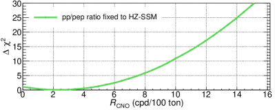
FIG. 11: $\Delta\chi^{2}$ profile for the $pep$ (top plot) and CNO (bottom plot) $\nu$ interaction rates.

As anticipated, the similarity between the $e^{-}$ recoil spectrum induced by the CNO neutrinos and the ²¹⁰Bi spectrum makes it impossible to disentangle the two contributions with the spectral fit without an external constraint on the ²¹⁰Bi rate. For this reason, we can only provide an upper limit on the CNO neutrinos interaction rate $R_{\rm{CNO}}$. In order to do so, we need further to break the correlation between the CNO and $pep$ contributions. In Phase-I, this was achieved by fixing the $pep$ $\nu$ rate to the theoretical value Bellini et al. (2012). In the current analysis, where $pp$ $\nu$s are included in the extended energy range of the fit, we place an indirect constraint on $pep$ $\nu$s by exploiting the theoretically well known $pp$ and $pep$ flux ratio. The interaction rate ratio $R_{pp}$/$R_{pep}$, is constrained to  (47.7 $\pm$ 0.8) (HZ) Vinyoles et al. (2017), Esteban et al. (2017). Constraining $R_{pp}$/$R_{pep}$ to the LZ hypothesis value 47.5 $\pm$ 0.8 gives identical results.

We carried out a sensitivity study by performing the analysis on thousands of data-sets simulated with the MC sensitivity tool: this study shows that under the current experimental conditions the total expected uncertainty (statistical plus systematical) is 3.4 cpd/100 ton. With this error, we expect the median 95% C.L. upper limit for $R_{\rm{CNO}}$ to be $\sim$ 9 cpd/100 ton and 10 cpd/100 ton, for low and high metallicity, respectively. On data, we obtain the upper limit on $R_{\rm{CNO}}$ = 8.1 cpd/100 ton (95 $\%$ C.L.) (see Table 2), which is slightly stronger than the median limit expected from the MC based sensitivity study. The $\Delta\chi^{2}$ profile for the CNO rate is shown in Fig. 11 (bottom). This result, using a weaker hypothesis on $pep$ $\nu$, confirms the current best limit on the flux of CNO $\nu$s previously obtained with Borexino Phase-I data Bellini et al. (2012).

VIII Conclusions

In summary, we have reported the details of the analyis and the results of the first simultaneous measurement of the $pp$, ⁷Be, and $pep$ components of the solar neutrino spectrum providing a comprehensive investigation of the main $pp$ chain in the Sun Agostini et al. (2018a). These results are in agreement with and improve the precision of our previous measurements. In particular, $R_{Be}$ is measured with an unprecedented precision of 2.7%. The absence of $pep$ neutrinos is rejected for the first time at more than 5$\,\sigma$. These data, together with our measurement about ⁸B $\nu$ flux in the HER Agostini et al. (2017a), provide a unique measurement of the interaction rates and thus of the fluxes of the different components of the solar neutrinos from the $pp$ chain with a single detector and a unified analysis approach.

The upper limit on $R_{\rm{CNO}}$ has the same significance as that of Borexino Phase-I and currently is providing the tightest bound on this component.

Several analysis methods and details here reported and discussed have a general interest which is going beyond the understanding of the Borexino results: as example the ¹¹C suppression, the multivariate fit, the analytical model of the energy response, the full MC description of the detector and the fitting procedures can be easily adapted to large volume liquid scintillator based detectors similar to Borexino Ciuffoli et al. (2013), Kraus (2006).

IX Acknowledgement

The Borexino program is made possible by funding from INFN (Italy), NSF (USA), BMBF, DFG, HGF, and MPG (Germany), RFBR (Grants 16-02-01026 A, 19-02-0097A, 16-29-13014 ofim, 17-02-00305 A)(Russia), RSF (grant 17-12-01009) (Russia), and NCN (Grant No. UMO 2013/10/E/ST2/00180-Grant No. UMO 2017/26/M/ST2/00915) (Poland). We acknowledge the computing services of Bologna INFN-CNAF data centre and LNGS Computing and Network Service (Italy), of Jülich Supercomputing Centre at FZJ (Germany), and of ACK Cyfronet AGH Cracow (Poland). We acknowledge also the generous hospitality and support of the Laboratori Nazionali del Gran Sasso (Italy).

References

- Fowler (1958) W. A. Fowler, The Astrophysical Journal 127, 551 (1958).
- Cameron (1958) A. W. G. Cameron, Annual Review of Nuclear Science 8, 299 (1958).
- Bahcall (2005) J. Bahcall, http://www.sns.ias.edu/j̃nb/SNdata (2005).
- Vinyoles et al. (2017) N. Vinyoles, A. M. Serenelli, F. L. Villante, S. Basu, J. Bergström, M. C. Gonzalez-Garcia, M. Maltoni, C. Peña-Garay, and N. Song, The Astrophysical Journal 835, 202 (2017).
- Anselmann et al. (1992) P. Anselmann et al. (GALLEX Collaboration), Physics Letters B 285, 376 (1992).
- Krauss (1992) L. M. Krauss, Nature 357, 437 (1992).
- Abdurashitov et al. (1994) J. N. Abdurashitov et al., Physics Letters B 328, 234 (1994).
- Cleveland et al. (1998) B. T. Cleveland et al., The Astrophysical Journal 496, 505 (1998).
- Fukuda et al. (1996) Y. Fukuda et al., Physical Review Letters 77, 1683 (1996).
- Abe et al. (2011) Y. Abe et al. (SuperKamiokande collaboration), Physical Review D 83, 052010 (2011).
- Ahmad et al. (2001) Q. R. Ahmad et al. (SNO collaboration), Physical Review Letters 87, 071301 (2001).
- Bellini et al. (2011a) G. Bellini et al. (Borexino Collaboration), Physical Review Letters 107, 141302 (2011a).
- Kajita and McDonald (2015) T. Kajita and A. B. McDonald, “The Nobel Prize in Physics 2015,” http://www.nobelprize.org/nobel_prizes/physics/laureates/2015 (2015).
- Jr. and Koshiba (2002) R. D. Jr. and M. Koshiba, “The Nobel Prize in Physics 2002,” http://www.nobelprize.org/nobel_prizes/physics/laureates/2002 (2002).
- Wolfenstein (1978) L. Wolfenstein, Physical Review D 17, 2369 (1978).
- Mikheev and Smirnov (1985) S. P. Mikheev and A. Y. Smirnov, Soviet Journal of Nuclear Physics 42, 913 (1985).
- Friedland et al. (2004) A. Friedland, C. Lunardini, and C. Peña-Garay, Physics Letters B 594, 347 (2004).
- Davidson et al. (2003) S. Davidson, C. Peña-Garay, N. Rius, and A. Santamaria, Journal of High Energy Physics 03 (2003).
- de Holanda and Smirnov (2004) P. C. de Holanda and A. Y. Smirnov, Physical Review D 49, 113002 (2004).
- Palazzo and Valle (2009) A. Palazzo and J. W. F. Valle, Physical Review D 80, 091301 (2009).
- Agostini et al. (2018a) M. Agostini et al. (Borexino Collaboration), Nature , 505 (2018a).
- Agostini et al. (2017a) M. Agostini et al. (Borexino Collaboration), https://arxiv.org/hep-ex/1709.00756 (2017a).
- Bellini et al. (2014a) G. Bellini et al. (Borexino Collaboration), Nature 512, 383 (2014a).
- Bellini et al. (2012) G. Bellini et al. (Borexino Collaboration), Physical Review Letters 108, 051302 (2012).
- Bellini et al. (2010) G. Bellini et al. (Borexino Collaboration), Physical Review D 82, 033006 (2010).
- Back et al. (2012) H. Back et al. (Borexino Collaboration), Journal of Instrumentation 7, P10018 (2012).
- Agostini et al. (2018b) M. Agostini et al. (Borexino Collaboration), Astroparticle Physics 97, 136 (2018b).
- Alimonti et al. (2009) G. Alimonti et al. (Borexino Collaboration), Nuclear Instruments and Methods A 600, 568 (2009).
- Bellini et al. (2014b) G. Bellini et al. (Borexino Collaboration), Physical Review D 89, 112007 (2014b).
- Bellini et al. (2011b) G. Bellini et al. (Borexino Collaboration), Journal of Instrumentation 6, P05005 (2011b).
- Franco et al. (2011) D. Franco, G. Consolati, and D. Trezzi, Physical Review C 83, 015504 (2011).
- Ding et al. (2018) X. F. Ding et al. (Borexino Collaboration), https://arxiv.org/abs/1805.11125 (2018).
- Agostinelli et al. (2003) S. Agostinelli et al., Nuclear Instruments and Methods A 506, 250 (2003).
- Agostini et al. (2017b) M. Agostini et al. (Borexino Collaboration), Astroparticle Physics 92, 21 (2017b).
- Agostini et al. (2015) M. Agostini et al. (Borexino), Phys. Rev. Lett. 115, 231802 (2015).
- Smirnov et al. (2016) O. Yu. Smirnov et al. (Borexino), Proceedings, 2nd International Workshop on Prospects of Particle Physics: Neutrino Physics and Astrophysics: Valday, Russia, February 1-8, 2015, Phys. Part. Nucl. 47, 995 (2016).
- Esteban et al. (2017) I. Esteban, M. C. Gonzalez-Garcia, M. Maltoni, I. Martinez-Soler, and T. Schwetz, Journal of High Energy Physics 01 (2017).
- Ciuffoli et al. (2013) E. Ciuffoli, J. Evslin, and X. Zhang, Phys. Rev. D 88, 033017 (2013).
- Kraus (2006) C. Kraus, Progress in Particle and Nuclear Physics 57, 150 (2006).