Polymer models with optimal good-solvent behavior

Abstract

We consider three different continuum polymer models, that all depend on a tunable parameter $r$ that determines the strength of the excluded-volume interactions. In the first model chains are obtained by concatenating hard spherocylinders of height $b$ and diameter $rb$ (we call them thick self-avoiding chains). The other two models are generalizations of the tangent hard-sphere and of the Kremer-Grest models. We show that, for a specific value $r^{*}$, all models show an optimal behavior: asymptotic long-chain behavior is observed for relatively short chains. For $r<r^{*}$, instead, the behavior can be parametrized by using the two-parameter model that also describes the thermal crossover close to the $\theta$ point. The bonds of thick self-avoiding chains cannot cross each other and, therefore, the model is suited for the investigation of topological properties and for dynamical studies. Such a model also provides a coarse-grained description of double-stranded DNA, so that we can use our results to discuss under which conditions DNA can be considered as a model good-solvent polymer.

I Introduction

In the last decades, a significant advancement in the theoretical understanding of polymeric systems has been possible thanks to the combination of simulative approaches Binder-96 , scaling arguments, and renormalization-group calculations deGennes-79 ; Freed-87 ; DE-88 ; dCJ-book ; Schaefer-99 . Most of the large-scale dynamic and static properties of synthetic homopolymers over a wide concentration range have been shown to be universal: the predictions of coarse-grained polymer models, often with only little connection to realistic systems, describe quite accurately the extensive experimental data collected from scattering, osmometric, and rheological experiments on chemically very different polymer solutions. This very successful approach has been applied to homopolymers of different topology and also extended to biopolymers; see, e.g., VFDLRRD-05 ; NYSK-13 ; TMDD-13 .

The physical appeal of the universal scaling picture relies on the possibility of formulating predictions invoking only a limited number of explanatory microscopic variables often connected to, and hence inferable from, experimentally accessible properties. For instance, the thermal crossover observed in dilute polymer solutions is typically parametrized using only a suitable combination of a microscopic excluded-volume parameter, expressing the average strength of the solvent-mediated monomer-monomer interaction, and the degree of polymerization deGennes-79 ; Freed-87 ; dCJ-book ; Schaefer-99 . This absence of tight constraints in the physical schematization of polymers has determined over the years the use, both in theory and simulations, of widely different coarse-grained chain models. Popular instances are the lattice self-avoiding walk model, the tangent hard-sphere (sometimes also named pearl-necklace) model DH-86 ; DH-88 and the Kremer-Grest GK-86 model. It is important to stress that only the large-scale behavior is universal, i.e., the behavior on length scales of the order of the radius of gyration $R_{g}$ or of de Gennes correlation length $\xi$ deGennes-79 , when they are significantly larger than any microscopic scale. Therefore, universality holds for long polymers in the dilute and semidilute regimes, but not for melts, in which the characteristic polymer length scales are in the microscopic domain (although in this case some scaling laws still hold). The universal behavior observed in the dilute and semidilute regimes can be rationalized using renormalization-group arguments, thanks to the de Gennes mapping deGennes-72 ; deGennes-79 ; dCJ-book of a polymer system onto a spin model, whose critical behavior is by now very well understood Wegner-76 ; PHA-91 ; PV-02 .

While universality is well established for the thermodynamic behavior of polymer solutions, the universality of the polymer dynamics is less clear. On general principles, one would expect a universal behavior on large time scales, i.e., for $t\gg\tau_{0}$, where $\tau_{0}$ is the Kuhn monomer relaxation time, which can be understood using the standard renormalization-group tools Oono-85 ; WDF-86 ; WF-86 ; SFO-85 ; SH-89 . However, any physical dynamics should include the condition of bond-noncrossability, which represents a nonlocal dynamical constraint. In the dilute regime, in which different polymers do not overlap, this constraint should not be crucial and thus universality is expected to hold. In the semidilute regime, the role of the constraint is less clear as polymers strongly overlap, although there is no entanglement as the monomer density is vanishingly small.

It must be noted that, although all models exhibit the same asymptotic behavior for a large number of monomeric units, when relatively short chains are used, they deviate systematically from each other, leading to a serious issue of interpretability of the results. A brute-force numerical solution of the problem consists in simulating long chains, which can be done quite efficiently for single isolated chains using clever algorithms developed in the years, see, e.g., Grassberger-97 ; Clisby-10-JSP . This is not feasible in finite-density simulations, in which typically the chain length never exceeds a few hundred monomeric units, making the quantitative comparison of different models rather difficult. For this reason, in the last years models rapidly approaching the universal large degree-of-polymerization limit have been proposed, see, for instance, BN-97 ; LK-99 ; CMP-06 ; DP-16 ; Clisby-17 . Alternatively, a number of first-principle coarse-grained approaches have been devised BLHM-01 ; MullerPlathe-02 ; PCH-07 ; PK-09 ; DPP-12-Soft ; DPP-12-JCP ; KVMP-12 ; Noid-13 , which reduce the complexity of the system by integrating out the short-scale degrees of freedom. Unfortunately, all these proposals, because of the lack of bond non-crossability, cannot be easily employed in dynamical studies (see PB-01 for an algorithmic way out), in which the topology or the concatenation properties of a chain must not change under any physical local dynamics. Beside the determination of polymer dynamical properties, this also represents a serious issue when looking at the knotting properties of macromolecules, which have gained a considerable attention in the last years OW-07 ; FSS-11 ; VRSWW-92 ; TRFM-13 ; EB-14 ; WC-86 ; VR-09 .

In this paper we wish to develop continuum polymer models that rapidly approach the universal scaling limit and that can, therefore, be used to investigate the thermodynamic properties of polymer solutions with a limited computational effort. It is important to note that the optimal interaction is obtained by studying the length dependence of specific observables for linear chains. However, the universality of subleading-amplitude ratios, which has been extensively verified in the context of spin systems AA-80 ; PV-02 ; PHA-91 , indicates that the cancellation of the leading finite-length corrections only depends on the specific nature of the interactions, while it is independent of the specific observable one is considering. Moreover, extensive numerical studies show that these finite-length corrections are not related to the polymer topology, and are always controlled by the same renormalization-group operator; for instance, the length dependence is specified by the same exponent $\Delta$ JRWM-90 ; FZ-11 ; HNG-04 ; RP-13 , which takes the value Clisby-10 $\Delta\approx 0.53$. Therefore, an optimal interaction for linear chains is also optimal when considering other types of polymer conformations. For star polymers this was explicitly verified in HNG-04 ; RP-13 . It should be noted that, for cyclic chains, renormalization-group theory guarantees the optimality of the models only if averages are taken over all chains, independently of the knot type. If one considers instead polymers of fixed knot type, the behavior is less clear, as new corrections might appear. This issue deserves additional investigations. The models we consider are also relevant for studies of mixtures of polymers and other nanoparticles, although in this case a fast convergence is only obtained by additionaly tuning the polymer-nanoparticle interactions DP-16 .

We will discuss three different models. First, we analyze the thick self-avoiding chain VLKFKC-92 ; RCV-93 ; VC-95 ; GM-99 ; SM-00 ; MPR-08 ; UD-15-17 ; PZC-16 , which has been studied at length in the past as a minimalistic model for double-stranded DNA filaments VLKFKC-92 ; RCV-93 ; VC-95 . Specifically, we determine the optimal thickness for which, under good-solvent (GS) conditions, the universal large degree-of-polymerization limit can be obtained for relatively short chains. As a byproduct of the calculation, we also determine the thickness crossover of the model, characterizing quantitatively the region between the ideal-chain limit and the GS behavior. The resulting behavior can be considered as representative of the one observed for DNA chains under various electrostatic screening conditions RCV-93 , at least in those cases in which the size of the chain is somewhat larger than the persistence length.

We also consider two popular models, often used to study the behavior of polymer solutions, the tangent hard-sphere model DH-86 ; DH-88 and the Kremer-Grest GK-86 model. We show that both of them exhibit very strong scaling corrections, so that results depend significantly on the number of monomers used. Both models can be easily generalized so that, by tuning a single parameter, one can obtain an optimal model, which approaches the asymptotic limit for small contour lengths. However, in the resulting optimal models bonds can cross each other. Therefore, they cannot be straightforwardly used in dynamical studies and whenever topology and concatenation are important.

The paper is organized as follows. In Sec. II we define the thick self-avoiding chains and discuss their relation with the models used in the description of double-stranded DNA and in the mathematical knot literature VLKFKC-92 ; RCV-93 ; VC-95 ; GM-99 ; MPR-08 . The thickness crossover and the behavior close to the GS regime are analyzed in Secs. III and IV, respectively. In Ref. V we extend the previous results to the tangent hard-sphere DH-86 ; DH-88 and to the Kremer-Grest GK-86 models. Finally, in Sec. VI we draw our conclusions. In the Appendix we compute the asymptotic expansion of an integral useful for the discussion of the Kremer-Grest model.

II Thick self-avoiding chains

Figure 1: The model. On the left, we show a typical chain of spherocylinders. We require that nonadjacent segments do not overlap, so $r_{\rm min}>d$, where $r_{\rm min}$ is the minimum distance between the axes of the two cylinders. Adjacent spherocylinders overlap, but the excluded-volume condition implies $\phi_{i}<\phi_{0}=\pi-2\arccos(d/2b)$.

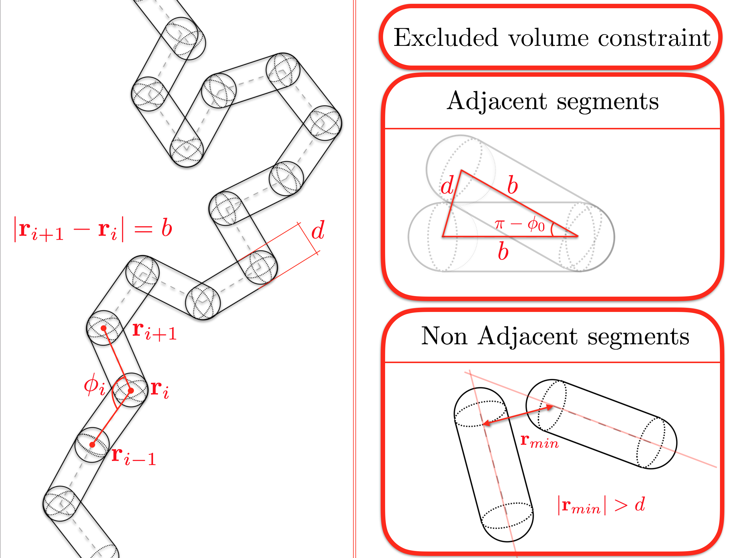We consider here a polymer model that has often been used to describe double-stranded DNA at a coarse-grained level VLKFKC-92 ; RCV-93 ; VC-95 . A polymer with $L$ monomers is modelled as a chain made by $L-1$ spherocylinders, see Fig. 1. Specifically, a chain is defined by $L$ points $\{{\bm{r}}_{1},\ldots,{\bm{r}}_{L}\}$ such that the distance between subsequent units is fixed, i.e., $|{\bm{r}}_{i}-{\bm{r}}_{i-1}|=b$. Excluded volume effects are accounted for by treating each segment connecting two successive points as the axis of a spherocylinder, i.e., of a hard cylinder of height $b$ and diameter (thickness) $d$, capped by two half spheres of radius $d/2$. Because of their steric encumbrance, nonadjacent spherocylinders cannot overlap. This condition is easily verified numerically, checking whether the minimum distance $r_{\rm min}$ between the axes of the two cylinders satisfies $r_{\rm min}>d$. Such distance can be computed using the fast algorithm of VL-94 . Successive spherocylinders can instead partly overlap. In the limit $d\to 0$ the excluded-volume constraint disappears and we obtain a freely-jointed chain.

The model we consider is very similar to that considered in the mathematical knot literature, see, e.g., GM-99 ; MPR-08 ; PZC-16 . The main difference concerns the local constraint between two successive units. A model that generalizes ours and that of GM-99 ; MPR-08 ; PZC-16 is obtained as follows. We define ${\bm{e}}_{i}={\bm{r}}_{i+1}-{\bm{r}}_{i}$ and the angle $\phi_{i}$ ($0\leq\phi_{i}\leq\pi$) as

$$\cos\phi_{i}={{\bm{e}}_{i}\cdot{\bm{e}}_{i+1}\over|{\bm{e}}_{i}||{\bm{e}}_{i+1}|}.$$ (1)

A more general model is obtained by requiring $\phi_{i}<\phi_{0}$, for some fixed $\phi_{0}$. In our model, the excluded volume requirement for nonadjacent spherocylinders implies $|{\bm{r}}_{i}-{\bm{r}}_{i-2}|>d$, so we have $\phi_{0}=\pi-2\arccos(d/2b)$. The model of GM-99 ; MPR-08 ; PZC-16 differs only in the value of $\phi_{0}$: they take $\phi_{0}=\pi-2\arccos(d/b)$.

Thick self-avoiding chains provide a coarse-grained model for double-stranded DNA, where $b$ may be identified with the Kuhn length RC-libro $l_{K}$ ($l_{K}$ is twice the persistence length), while $d$ is an effective thickness, that depends on the amount of salt (pH) present in the solution RCV-93 ; VC-95 . In principle, by tuning the angle $\phi_{0}$ defined above, we can also obtain a more accurate description in which $b<l_{K}$ and each spherocylinder represents a shorter DNA segment. Alternatively, one can introduce a bending energy $E_{b}=\alpha\sum_{i}(1-\cos\phi_{i})$, as in VLKFKC-92 ; RCV-93 ; VC-95 , depending on a bending parameter $\alpha$.

Depending on the value of $d$, finite-length polymers can exhibit a different behavior. For small values of the thickness $d$, i.e., for very small excluded-volume interactions, the behavior is very similar to that of $\theta$-point chains. As $d$ increases, excluded-volume interactions become more effective, and therefore the behavior becomes gradually closer to that expected for a GS polymer. Therefore, the thickness $d$ plays the same role as that of the temperature $T$ in the analysis of the thermal crossover between the $\theta$ and the GS regime of homopolymer solutions. In that context, solvent quality is usually parameterized by using the Zimm-Stockmayer-Fixmann variable ZSF-53 $z\sim(T-T_{\theta})L^{1/2}$, where $T_{\theta}$ is the $\theta$ temperature. The $\theta$ behavior is observed for $z\approx 0$, while the GS regime is reached in the limit $z\to\infty$. We will show here that an analogous quantity can be defined for thick chains, replacing the temperature difference with an appropriate function of $d$. This allows us to map the crossover due to the change of the steric encumbrance on the standard thermal crossover, for which a wealth of theoretical and numerical results are available Yamakawa-71 ; Schaefer-99 ; dCJ-book ; CMP-08 ; DPP-13-Thermal .

To study the crossover, we perform Monte Carlo simulations of isolated chains for values of $d/b$ ranging from 0.0125 to 0.7 and polymer lengths $L$ from $250$ to $8000$. We use a continuum generalization of the pivot algorithm MS-88 , implementing the Kennedy algorithm Kennedy-02 to speed up the self-intersection check. We compute the second virial coefficient $B_{2}$ and the radius of gyration $R_{g}$. Then, we consider the universal combination $A_{2}=B_{2}R_{g}^{-3}$, which vanishes in the noninteracting case ($d=0$) and takes the value CMP-06 ; DP-16 $A_{2,GS}\approx 5.501$ for polymers under GS conditions. The interpenetration ratio $\Psi$ often used in the experimental literature is defined Yamakawa-71 ; Schaefer-99 ; dCJ-book as $\Psi={1\over 4}\pi^{-3/2}A_{2}$. We also consider the expansion (swelling) ratio $\alpha^{2}_{g}$ defined as the ratio between $R_{g}^{2}$ and the corresponding value for a freely jointed (ideal) chain of $L$ sites:

$$R^{2}_{g,0}=\frac{Lb^{2}}{6}\left(1-\frac{1}{L^{2}}\right).$$ (2)

III Thickness crossover

Figure 2: Second-virial combination $A_{2}$ vs $d/b$ for several values of the chain length $L$. The horizontal line corresponds to the good-solvent value $A_{2,GS}=5.501$.

Figure 3: Plot of $\Delta\nu=\nu_{\rm eff}-\nu_{GS}$, for several values of the chain lengths ($L_{1}$, $L_{2}$).

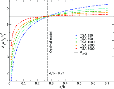
In Fig. 2 we report the second-virial combination $A_{2}$ versus the thickness $d$. The observed behavior is completely analogous to that observed in experimental systems (see, e.g., Berry-66 and the recent reanalysis presented in the supplementary material of DPP-14-GFVT ) or in Monte Carlo simulations of polymer models PH-05 , once we replace $d/b$ with $T-T_{\theta}$. At fixed $d\not=0$ the estimates of $A_{2}$ converge to the GS value as $L\to\infty$, with discrepancies that increase as $d$ decreases towards zero. For $d/b\approx 0.27$ we obtain GS behavior even for small values of $L$. For $d/b\mathrel{\hbox to0.0pt{\lower 3.0pt\hbox{$\mathchar 536\relax$}\hss}\raise 2.0pt\hbox{$\mathchar 316\relax$}}0.27$ the approach to the GS value is from below, while for larger values of $d/b$ the finite-$L$ estimates are larger than the asymptotic value. Finite-length corrections to the GS behavior are therefore both positive and negative, a phenomenon well documented in the thermal case Schaefer-99 ; KS-94 .

It is also interesting to discuss how the size of the chain changes with $L$ for different values of $d/b$. For this purpose, we define an effective Flory exponent $\nu_{\rm eff}$,

$$\nu_{\rm eff}(d/b;L_{1},L_{2})={\ln[R_{g}(d/b;L_{1})/R_{g}(d/b;L_{2})]\over\ln(L_{1}/L_{2})}.$$ (3)

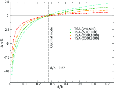
In the good-solvent limit we should find $\nu_{\rm eff}=\nu_{GS}$, where $\nu_{GS}$ is the universal good-solvent exponent, which is known with high accuracy Clisby-10 : $\nu_{GS}=0.587597(7)$. In Fig. 3 we report $\Delta\nu=\nu_{\rm eff}-\nu_{GS}$ for several pairs $(L_{1},L_{2})$. The results are analogous to those shown in Fig. 2. For $d/b<0.27$, the effective exponent is smaller than $\nu_{GS}$ and increases toward the good-solvent value as $L_{1}$ and $L_{2}$ increase. For $d/b>0.27$ the opposite occurs, while for $d/b\approx 0.27$, the radius of gyration scales quite precisely as $L^{\nu_{GS}}$.

We will now show that the crossover for $d/b\mathrel{\hbox to0.0pt{\lower 3.0pt\hbox{$\mathchar 536\relax$}\hss}\raise 2.0pt\hbox{$\mathchar 316\relax$}}0.27$, interpolating between ideal and GS behavior, can be parametrized by using the standard two-parameter model (TPM) scaling functions Yamakawa-71 ; dCJ-book ; Schaefer-99 . For this purpose we define the scaling variable $z$ as $z=av(d/b)L^{1/2}$, where the excluded-volume parameter $v(d/b)$ is identified with Hall-80 the adimensional microscopic virial coefficient—the one associated with the interaction of two isolated monomers. For pairs of identical spherocylinders we have Isihara-50 ; IH-51 ; Kihara-53

$$v(d/b)=\frac{2\pi}{3}{d^{3}\over b^{3}}\left(1+\frac{3b}{2d}+\frac{3b^{2}}{8d^{2}}\right).$$ (4)

The constant $a$ is fixed by the convention that $\Psi\approx z$ for $z\to 0$.

In order to determine $a$, we performed simulations for small values of $z$ for $L=1000$, corresponding to values of $A_{2}$ in the interval 0.5-1.5. We finally fitted the results (they are reported in Table 1) to the accurate TPM expression of CMP-08 :

$$A_{2}(z) = 4\pi^{3/2}zf_{2}(z)^{-1/4}$$ (5)

$$f_{2}(z) = 1+$$

$$268.96z^{4}+331.99z^{3}+126.783z^{2}+19.1187z.$$

We find $a\approx 0.647(2)$. As a consistency check we can compare the estimated $\alpha_{g}$ with the TPM prediction CMP-08 ,

$$\alpha_{g}(z)=(1+10.9288z+35.1869z^{2}+30.4463z^{3})^{0.0583867}.$$ (6)

The results are reported in Table 1: deviations are small, of less than approximately 1%.

Table 1: Monte Carlo estimates of $A_{2}$ and $\alpha^{2}_{g}$ for several values of $d$ and $L=1000$. For each $d/b$ and $L$ we compute $z$ using $z=0.647v(d/b)L^{1/2}$ and report the corresponding TPM predictions [we use Eqs. (5) and (6)].

$d/b$	$z$	$A_{2}$	$A_{2,TPM}$	$\alpha^{2}_{g}$	$\alpha^{2}_{g,TPM}$
0.00160	0.02582	0.516(1)	0.513	1.0302(3)	1.032
0.00253	0.04105	0.772(1)	0.767	1.0463(3)	1.049
0.00358	0.05838	1.024(1)	1.022	1.0640(3)	1.069
0.00476	0.07796	1.275(2)	1.276	1.0825(3)	1.089
0.00609	0.10031	1.524(2)	1.529	1.1036(3)	1.112

Figure 4: Second virial combination $A_{2}$ versus $\alpha^{2}_{g}$. We report the numerical results for several values of $L$, the extrapolations (see Table 2) of data at fixed $z$ and the TPM predictions from CMP-08 . In the inset we report $A_{2}$ versus $z=0.647v(d/b)L^{1/2}$.

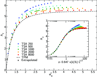In Fig. 4 we compare the TPM crossover curves with the whole set of Monte Carlo data. The results for $A_{2}$ are well reproduced up to $A_{2}\approx 5$, while larger discrepancies are observed for the swelling ratio, a phenomenon already observed in the analysis of the experimental data Berry-66 ; DPP-14-GFVT , which is due to the fact that the corrections to the GS behavior increase as $z\to\infty$.

Table 2: Crossover behavior in the spherocylinder model. We perform runs at values of $d/b$ such that $A_{2,TPM}(z)=1,2,3,4,5$, where $A_{2,TPM}(z)$ is given in Eq. (5) and $z=0.647v(d)L^{1/2}$. We report the estimates of $A_{2}$ and $\alpha_{g}^{2}$ for several values of $L$ and the corresponding large-$L$ extrapolation (we assume DJ-72 ; CMP-08 ; BN-97 $A_{2,L}=A_{2,\rm extr}+b_{1}L^{-1/2}+b_{2}/L$). Finally $\Delta=100(1-B_{\rm Extr}/B_{TPM})$, $B=A_{2}$ or $\alpha_{g}^{2}$.

$z$	$A_{2,TPM}(z)$	250	500	1000	2000	4000	Extr.	$\Delta\%$
0.056778	1	0.990(1)	0.992(2)	1.005(4)	1.002(8)	1.010(9)	1.03(2)	3
0.151493	2	1.958(2)	1.972(3)	1.994(6)	2.00(1)	2.00(1)	2.04(2)	2
0.331075	3	2.929(2)	2.936(2)	2.962(6)	2.97(1)	2.97(2)	3.03(3)	1.1
0.767908	4	3.934(3)	3.931(5)	3.944(8)	3.94(1)	3.96(2)	4.02(3)	0.4
3.01381	5	5.154(3)	5.045(5)	5.009(9)	4.97(2)	4.98(2)	4.99(3)	0.1
$z$	$\alpha^{2}_{g,TPM}(z)$	250	500	1000	2000	4000	Extr.
0.056778	1.0668	1.0572(2)	1.0604(4)	1.0616(7)	1.065(1)	1.061(2)	1.063(3)	0.35
0.151493	1.1602	1.1314(2)	1.1395(4)	1.1461(7)	1.149(1)	1.155(2)	1.1625(25)	0.2
0.331075	1.3020	1.2356(2)	1.2522(4)	1.2663(7)	1.276(1)	1.283(2)	1.304(3)	0.15
0.767908	1.5553	1.4028(2)	1.4364(4)	1.4627(7)	1.4859(1)	1.503(2)	1.544(3)	0.7
3.01381	2.2857	1.8237(3)	1.8913(5)	1.9538(9)	2.010(2)	2.057(2)	2.172(5)	5

A more detailed check is presented in Table 2. Here we consider five different values of $z$ such that $A_{2,TPM}(z)$ is 1,2,3,4,5, respectively, and several values of $L$. For each $z$ and $L$, we compute the corresponding value of $d/b$. Then, we perform simulations of chains of length $L$ with the computed $d/b$. As it can be seen from Table 2, results show only a tiny dependence on $L$. Moreover, the extrapolated large-$L$ values are consistent with the TPM predictions, both for $A_{2}$ and for the swelling ratio. Only in one case, the result for $\alpha^{2}_{g}$ at $z=3.01381$, do we observe a significant difference. This may be due to additional corrections to scaling that are not taken into account in the extrapolation (if we do not use the result for $L=250$, the extrapolated value becomes 2.190(7), which is closer to the TPM estimate) and to the inaccuracy of Eq. (6)—the interpolation should be accurate at the level of a few percent.

It is important to stress that, if we change the model by considering a different value of $\phi_{0}$ (the parameter that controls the interaction of two successive spherocylinders) or by adding a bending energy as in DNA models, only the constant $a$ entering the definition of $z$ changes. The TPM describes the crossover behavior of any large-scale quantity for any model parameter, provided the constant $a$ is appropriately chosen.

Figure 5: Estimates of the two-body potential as a function of $r/R_{g}$. We report Monte Carlo results (points) for spherocylinder chains with $L=4000$ monomers at values of $d/b$ such that $A_{2}(z_{n})=n$ and the results (lines) of DPP-13-Thermal obtained by using the lattice Domb-Joyce model. Data labelled “Optimal GS L=250” (points) correspond to simulations of $L=250$ chains for $d/b=0.275$ (the optimal model discussed in Sec. IV). The line that goes through these data was obtained in PH-05 , by extrapolating self-avoiding walk results.

Figure 6: Estimates of the three-body potential for equilateral configurations for the same values of $d/b$ and $L$ as in Fig. 5. In the main frame, the lines going through the points are only meant to guide the eye. The data labelled “SAW” in the inset were obtained in DPP-compressible by using the lattice Domb-Joyce model.

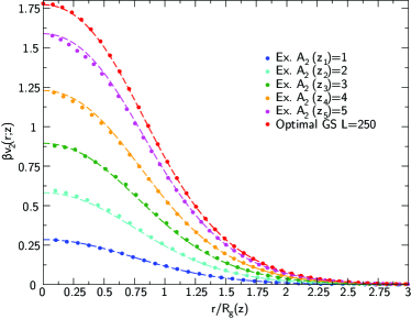
To verify the correctness of our parametrization of the steric crossover, we consider two other quantities, which characterize the intermolecular structure of a polymer solution in the dilute regime. We compute the effective center-of-mass two-body and three-body potential BLHM-01 ; Louis . In Fig. 5 we report our results for five different values of $d/b$ chosen so that $A_{2,TPM}(z_{n})=n$ (the same values of $z$ considered in Table 2) and compare them with those obtained in DPP-13-Thermal , using the lattice Domb-Joyce model DJ-72 . We observe a very good agreement, confirming that we have correctly identified the scaling variable $z$. In Fig. 6 we show the corresponding three-body center-of-mass potentials, which, as expected, converge to zero as $z$ goes to zero. Again, they agree with those obtained by using the lattice Domb-Joyce model DPP-compressible .

IV Good-solvent behavior and optimal model

In the previous section we have discussed the crossover behavior for small values of $d$, up to $d/b\approx 0.27$, where GS behavior is observed even for small values of $L$. We wish now to focus on the behavior close to this value of $d$. In general, for large values of $L$, any generic large-scale adimensional quantity $A$, which depends on $L$ and $d$, behaves as

$$A(L,d)=A_{GS}+a_{1,A}(d)/L^{\Delta}+a_{2,A}(d)/L^{\Delta_{2}}+\ldots$$ (7)

where $A_{GS}$ is universal, i.e., independent of $d$. The exponent $\Delta$ is also universal [simulations of self-avoiding walks give Clisby-10 $\Delta=0.528(12)$], and so is $\Delta_{2}\approx 1$. The amplitudes $a_{1,A}(d)$ and $a_{2,A}(d)$ depend instead on the model. However, given two different observables $A$ and $B$, the amplitude ratios $a_{1,A}(d)/a_{1,B}(d)$ are model independent AA-80 .

Finite-length corrections represent the main obstacle for a precise determination of the leading, universal behavior under GS conditions. However, one can exploit the model dependence of the corrections to identify optimal models for which the leading scaling corrections vanish. In our case, we wish to determine the value $d^{*}$ of the thickness parameter, for which the leading scaling corrections vanish. Note that, if $a_{1,A}(d^{*})=0$ for a given observable $A$, the universality of the amplitude ratios implies that $a_{1,B}(d^{*})=0$ for any other observable $B$.

Figure 7: Top: Scaling correction coefficient $a_{1}(d)$ versus $d/b$; the line is the linear interpolation. Bottom: $A_{2}(d,L)/A_{2,GS}$ versus $L^{-\Delta}$, $\Delta=0.528$, for several values of $d/b$.

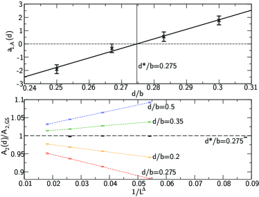To determine $d^{*}$, we consider $A_{2}(d,L)$. We fit $A_{2}(d,L)-A_{2,GS}$ to

$${a_{1}(d)\over L^{\Delta}}+{a_{2}(d)\over L^{\Delta_{2}}},$$ (8)

fixing $A_{2,GS}=5.500$, $\Delta=0.528$ and $\Delta_{2}=1$. We repeat the procedure for several values of $b$ in the interval $0.25\leq d/b\leq 0.30$, obtaining estimates of $a_{1}(d)$ that are fitted to $a_{1}(d)=c(d-d^{*})$. We obtain

$$d^{*}/b=0.275(2),$$ (9)

where the error takes into account the variation of the estimates if $\Delta$ varies by Clisby-10 0.012 and $\Delta_{2}$ by 0.1. We have then performed simulations for such a value of $d/b$. The results reported in Table 3 completely confirm the analysis. It is important to note that the estimate of $d^{*}/b$ is strictly model dependent, and therefore a different result would be obtained if the model is changed by adding, for instance, a bending interaction term or by considering a different value for the parameter $\phi_{0}$ that controls the interaction between two adjacent spherocylinders.

Table 3: Second-virial combination $A_{2}$, asphericity $A_{\rm sph}$, ratios $L_{3,1}$ and $L_{2,1}$ between the eigenvalues of the gyration tensor, and ratio $A_{ge}$, for $d/b=0.275$ and several values of $L$. The extrapolated ($L=\infty$) value of $A_{2}$ is taken from DP-16 , those for the shape factors are extrapolations of the results of Sciutto-96 , while the estimate of $A_{ge}$ is taken from Clisby-10 .

$L$	$A_{2}$	$A_{\rm sph}$	$L_{3,1}$	$L_{2,1}$	$A_{ge}$
100	5.478(1)	0.42962(3)	13.821(2)	2.9222(4)	0.16093(6)
250	5.494(1)	0.43054(3)	13.908(2)	2.9351(5)	0.16020(6)
500	5.497(2)	0.43062(5)	13.925(3)	2.9393(6)	0.16006(6)
1000	5.491(4)	0.4305(1)	13.923(7)	2.940(1)	0.1599(2)
$\infty$	5.5007(14)	0.4302(9)	13.92(6)	2.934	0.15991(5)

To verify that the leading scaling corrections are absent in any observable for $d/b\approx 0.275$, we consider other observables. First, we check that the radius of gyration scales as $L^{\nu_{GS}}$ with tiny corrections. If we use the numerical result $R_{g}=20.882(4)$ for $L_{1}=1000$ and Clisby-10 $\nu_{GS}=0.587597$, we predict for $L_{2}=100$

$$R_{g}(L_{2})=R_{g}(L_{1})\left({L_{2}\over L_{1}}\right)^{\nu_{GS}}\approx 5.397,$$ (10)

which is in excellent agreement with the direct numerical estimate $R_{g}(L_{2})=5.3901(4)$. At the optimal value of $d/b$, the scaling $R_{g}\sim L^{\nu_{GS}}$ holds therefore with a 0.1% error already for $L=100$. As an additional check, we have measured some adimensional quantities related to the polymer shape. If $\lambda_{1}\leq\lambda_{2}\leq\lambda_{3}$ are the eigenvalues of the gyration tensor, we consider Sciutto-96 ; shape ; Causo-02 the asphericity $A_{\rm sph}$

$$A_{\rm sph}=\left\langle{\lambda_{1}^{2}+\lambda^{2}_{2}+\lambda^{2}_{3}-\lambda_{1}\lambda_{2}-\lambda_{1}\lambda_{3}-\lambda_{2}\lambda_{3}\over(\lambda_{1}+\lambda_{2}+\lambda_{3})^{2}}\right\rangle$$ (11)

and the ratios $L_{12}=\langle\lambda_{2}\rangle/\langle\lambda_{1}\rangle$, $L_{13}=\langle\lambda_{3}\rangle/\langle\lambda_{1}\rangle$. Finally, we also consider the ratio $A_{ge}=R^{2}_{g}/R_{e}^{2}$, where $R^{2}_{e}$ is average squared end-to-end distance. Results are reported in Table 3. The $L$-dependence is tiny and significantly smaller than that observed for lattice self-avoiding walks (SAWs) Sciutto-96 ; shape ; Causo-02 , for which scaling corrections are large. Extrapolations give results that are consistent with the extrapolated SAW results. As a final check we have also computed the effective two-body and three-body center-of-mass effective potentials BLHM-01 ; Louis , see Figs. 5 and 6. The results for the two-body potentials can be compared with those obtained for SAWs (extrapolations of results for chains of length up to $L=4000$) BLHM-01 ; PH-05 , and with the ones DPP-compressible obtained by using the lattice Domb-Joyce model DJ-72 . We observe perfect agreement, already for chains of $L=250$ monomers. The same holds for the three-body potential on equilateral configurations.

V Comparison with other popular continuum models

Figure 8: Second-virial combination $A_{2}$ vs $L^{-\Delta}$, $\Delta=0.528$, for the KG model with $\beta\epsilon_{nb}=4$ (KG) and for the THSM with $d=b$ (THSM). For comparison, we also report results for the self-avoiding walk (SAW) model on a cubic lattice. The asymptotic estimate is $A_{2}^{*}=5.5007$ DP-16 . On the left we report the relative deviation $(A_{2}-A_{2}^{*})/A^{*}_{2}$ in %.

Figure 9: Crossover behavior of the generalized hard-sphere model. Top: $A_{2}$ versus $d/b$ for several values of $L$. Bottom: $A_{2}$ versus $\alpha^{2}_{g}$ and (inset) $A_{2}$ versus $z$. The same data in the spherocylinder case are shown in Figs. 2 and 4.

In the analysis of the behavior of polymer solutions, two other models are commonly used, the tangent-hard sphere model (THSM) DH-86 ; DH-88 , and the Kremer-Grest (KG) model GK-86 . As we shall show, these models exhibit very large finite-length corrections, so values of $L$ of the order of $10^{3}$ are required to obtain results that differ from the asymptotic ones by less than 10%. Both models can be generalized. By tuning a single parameter that plays the same role as the thickness $d$, one can define optimal models that show GS behavior for small values of $L$. Moreover, also these generalized models can be used to describe the thermal crossover. However, because different bonds can cross each other, they cannot be easily employed to study the polymer dynamics or topological properties.

V.1 Definition of the generalized models

The generalization of the THSM is defined as follows. A chain of $L$ monomers is a random walk $\{{\bm{r}}_{1},\ldots,{\bm{r}}_{L}\}$, such that $|{\bm{r}}_{i}-{\bm{r}}_{i+1}|=b$ ($b$ is therefore the bond length) for all successive monomers. Each monomer is modelled as a hard sphere of diameter $d$, so that $|{\bm{r}}_{i}-{\bm{r}}_{j}|>d$ if $|i-j|>1$. The THSM is obtained by setting $d=b$. In the generalized model, by decreasing $b/d$, one can increase the stiffness of the polymers. The angle $\phi_{i}$ defined in (1) is always smaller than $\phi_{0}$, with $\phi_{0}\to 180^{\circ}$ for $b/d\to\infty$ (completely flexible chains), $\phi_{0}=120^{\circ}$ for $b/d=1$ and $\phi_{0}\to 0$ as $b/d\to 1/2$ (rod limit). Because of this property, such a model has already been used to model semiflexible protein chains SHG-16 .

A generalization of the KG model is obtained by considering different Lennard-Jones potentials for the bonding and non-bonding interactions. To be precise, we define the truncated and shifted Lennard-Jones potential

$$V_{LJ}(r,\epsilon)=\begin{cases}\epsilon\left[\left({\sigma\over r}\right)^{12}-\left({\sigma\over r}\right)^{6}+{1\over 4}\right]&\qquad\mbox{for }{r\over\sigma}<2^{1/6},\\ 0&\qquad\mbox{for }{r\over\sigma}\geq 2^{1/6}\end{cases}$$ (12)

and

$$V_{\rm FENE}(r,\epsilon_{F})=\begin{cases}-\epsilon_{F}\left({b_{0}\over\sigma}\right)^{2}\ln\left(1-{r^{2}\over b_{0}^{2}}\right),&\qquad r<b_{0}\\ +\infty&\qquad r\geq b_{0}.\end{cases}$$ (13)

In the generalization of the KG model, bonded monomers interact with potential

$$V_{\rm bond}(r)=V_{LJ}(r,\epsilon_{b})+V_{\rm FENE}(r,\epsilon_{F}),$$ (14)

where $r=|{\bm{r}}_{i}-{\bm{r}}_{i+1}|$. Parameters $\epsilon_{b}$, $\epsilon_{F}$ and $b_{0}$ are chosen as in GK-86 : $\beta\epsilon_{b}=4$, $\beta\epsilon_{F}=15$, $b_{0}/\sigma=1.5$. This choice guarantees that the typical bond length $b$ is approximately $\sigma$ (simulations indicate that $b\approx 0.97\sigma$ for an isolated chain for all different nonbonded interactions we have considered). For nonbonded monomers we consider instead

$$V_{\rm nonbond}(r)=V_{LJ}(r,\epsilon_{nb}),$$ (15)

with the same $\sigma$, but with a different $\epsilon_{nb}$. The usual KG interaction is obtained for $\epsilon_{nb}=\epsilon_{b}$.

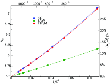
The THSM and the standard KG models show significant finite-length corrections, as it can be seen in Fig. 8, where we report $A_{2}$ as a function of $L$. The data clearly approach the asymptotic value CMP-06 ; DP-16 $A_{2,GS}\approx 5.50$. More quantitatively, if we fit the KG data at $\beta\epsilon_{nb}=4$ to $a+b/L^{\Delta}+c/L$, with $\Delta=0.528$, we obtain $a=5.498(15)$, in perfect agreement with the lattice result. However, in these models $A_{2}$ approaches the limiting value quite slowly: the relative difference $A_{2}/A_{2,GS}-1$ is less than 10% only for $L\mathrel{\hbox to0.0pt{\lower 3.0pt\hbox{$\mathchar 536\relax$}\hss}\raise 2.0pt\hbox{$\mathchar 318\relax$}}10^{3}$. Similar results are obtained for the THSM DP-16 . Note that, for a given value of $L$, the two models give very close estimates of $A_{2}$. This can be rationalized by using the Barker-Henderson BH-67 mapping of the KG model onto the THSM. In this approach the KG model is equivalent to the generalization of the THSM with $b\approx 0.97\sigma$ and hard-sphere diameter

$$d_{BH}=\int_{0}^{\infty}dr\,(1-e^{-\beta V_{LJ}(r,\epsilon_{nb})}).$$ (16)

For $\beta\epsilon_{nb}=4$ we obtain $d_{BH}=1.01\sigma\approx 1.04b$. The bond length and the hard-sphere diameter are approximately the same, so the KG model is essentially equivalenty to the THSM.

As $A_{2}(L)$ in both models is larger than $A_{2,GS}$, an optimal model is obtained by reducing the strength of the nonbonding potential, i.e., by increasing $b/d$ or decreasing $\beta\epsilon_{nb}$. This analysis will be presented below.

V.2 Generalized hard-sphere model

Table 4: Crossover behavior in the generalized hard-sphere model. We perform runs at values of $d/b$ such that $A_{2,TPM}(z)=1,2,3,4,5$, where $A_{2,TPM}(z)$ is given in Eq. (5) and $z=0.669v_{HS}(d)L^{1/2}$. We report the estimates of $A_{2}$ and $\alpha_{g}^{2}$ for several values of $L$ and the corresponding large-$L$ extrapolation (we assume DJ-72 ; CMP-08 ; BN-97 $A_{2,L}=A_{2,\rm extr}+b_{1}L^{-1/2}+b_{2}/L$). Finally $\Delta=100(1-B_{\rm Extr}/B_{TPM})$, $B=A_{2}$ or $\alpha_{g}^{2}$.

$z$	$A_{2,TPM}(z)$	250	500	1000	2000	4000	Extr.	$\Delta\%$
0.056778	1	1.011(1)	1.006(2)	0.993(4)	0.984(8)	0.991(3)	0.980(8)	2
0.151493	2	2.091(2)	2.055(3)	2.027(6)	2.02(1)	2.003(5)	1.98(1)	2
0.331075	3	3.253(3)	3.166(4)	3.108(7)	3.07(1)	3.037(6)	2.97(1)	3
0.767908	4	4.507(3)	4.340(4)	4.224(8)	4.146(15)	4.093(6)	3.96(2)	1
3.01381	5	5.854(3)	5.580(4)	5.388(8)	5.27(1)	5.187(6)	4.99(2)	0.2
	$\alpha^{2}_{g,TPM}(z)$	250	500	1000	2000	4000	Extr.
0.056778	1.0668	1.0627(2)	1.0638(3)	1.0659(6)	1.0668(13)	1.0673(6)	1.070(1)	0.32
0.151493	1.1602	1.1474(2)	1.1516(3)	1.1543(6)	1.1591(13)	1.1583(6)	1.163(1)	0.2
0.331075	1.3020	1.2785(2)	1.2865(3)	1.2916(7)	1.2937(13)	1.2967(6)	1.301(1)	0.1
0.767908	1.5553	1.5249(2)	1.5371(4)	1.5445(7)	1.5481(13)	1.5503(6)	1.555(1)	0.0
3.01381	2.2857	2.3201(3)	2.3222(5)	2.3233(8)	2.319(2)	2.3136(7)	2.303(5)	0.8

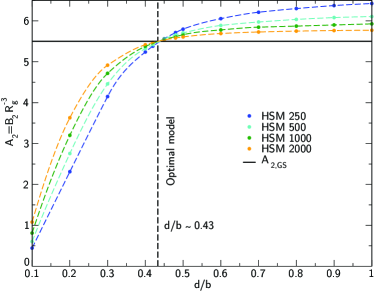
We consider first the hard-sphere model, repeating the analysis presented in Sec. IV. Simulations show different regimes, see the top panel of Fig. 9, which are completely analogous to those observed for spherocylinders. For $d/b\mathrel{\hbox to0.0pt{\lower 3.0pt\hbox{$\mathchar 536\relax$}\hss}\raise 2.0pt\hbox{$\mathchar 316\relax$}}0.43$, there is a clear crossover between the ideal and the GS behavior. For $d/b\approx 0.43$, the $L$ dependence is tiny, while, for $d/b\mathrel{\hbox to0.0pt{\lower 3.0pt\hbox{$\mathchar 536\relax$}\hss}\raise 2.0pt\hbox{$\mathchar 318\relax$}}0.43$, $A_{2}$ is larger than $A_{2,GS}$ for finite values of $L$. The crossover behavior for $d/b\mathrel{\hbox to0.0pt{\lower 3.0pt\hbox{$\mathchar 536\relax$}\hss}\raise 2.0pt\hbox{$\mathchar 316\relax$}}0.43$ can be parametrized by using the variable $z$, which is now defined as $z=a_{HS}v_{HS}(d/b)L^{1/2}$, where $v_{HS}(d/b)={2\pi\over 3}d^{3}/b^{3}$ is the adimensional monomer-monomer second-virial coefficient. The constant $a_{HS}$ is again fitted so as to reproduce the data for small values of $z$. Using data obtained from simulations of chains with $L=1000$, we obtain $a_{HS}=0.669(2)$. As in the spherocylinder case, the TPM curves describe quite well the crossover up to $A_{2}\approx 5$, see Fig. 9, while larger discrepancies are observed for larger values. We also perform a detailed check for a few selected values of $z$. The results, shown in Table 4, confirm the identification of the $z$ variable. In all cases, the extrapolated (large-$L$) results are consistent with the TPM predictions.

Figure 10: Top: Scaling correction coefficient $a_{1}(d)$ versus $d/b$ for the generalized hard-sphere model; the line is the linear interpolation. Bottom: $A_{2}(d,L)/A_{2,GS}$ versus $L^{-\Delta}$, $\Delta=0.528$, $A_{2,GS}=5.500$, for several values of $d/b$.

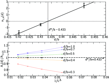We also determined the optimal model for which there are no leading finite-length corrections. For this purpose, we performed simulations of chains of length 250, 500, 1000, and 2000 for $d/b=0.42,0.43,0.45$. Fits to Eq. (8) give estimates of $a_{1}(d/b)$. Performing a linear interpolation, see Fig. 10, we obtain

$$d^{*}/b=0.433(1).$$ (17)

This result compares well with the estimate $d^{*}/b\approx 0.447$ of LK-99 .

Table 5: Second-virial combination $A_{2}$, asphericity $A_{\rm sph}$, ratios $L_{3,1}$ and $L_{2,1}$ between the eigenvalues of the gyration tensor, and ratio $A_{ge}$, for the optimal hard-sphere model with $d/b=0.433$ and several values of $L$. The extrapolated value of $A_{2}$ is taken from DP-16 , those for the shape factors are extrapolations of the results of Sciutto-96 , while the estimate of $A_{ge}$ is taken from Clisby-10 .

$L$	$A_{2}$	$A_{\rm sph}$	$L_{3,1}$	$L_{2,1}$	$A_{ge}$
100	5.430(3)	0.42757(5)	13.691(4)	2.9061(7)	0.16137(5)
250	5.475(4)	0.42930(7)	13.824(5)	2.9249(9)	0.16049(7)
500	5.478(4)	0.42994(9)	13.875(6)	2.9321(12)	0.16024(8)
1000	5.509(8)	0.4301(2)	13.890(11)	2.935(2)	0.1601(1)
$\infty$	5.5007(14)	0.4302(9)	13.92(6)	2.934	0.15991(5)

As we have already mentioned, in the optimal model any observable should not present scaling corrections decaying as $L^{-\Delta}$, guaranteeing a faster convergence to the infinite-length limit. To verify this cancellation, we consider again the shape factors. Results for the hard-sphere model are reported in Table 5. They should be compared with those appearing in Table 3 for the spherocylinder model. Also in the hard-sphere case do we observe a fast convergence (discrepancies are well explained by corrections decaying as $1/L$). As for the next-to-leading corrections, the optimal spherocylinder model performs better than the hard-sphere one.

Table 6: Estimates of $A_{2}$ as a function of the non-bonding LJ parameter $\beta\epsilon_{nb}$ and of $L$ for the generalized Kremer-Grest model. Here $d_{BH}$ is the Barker-Henderson effective diameter [for small values of $\epsilon_{nb}$, one can use the asymptotic expression $d_{BH}/\sigma\approx(\beta\epsilon_{nb})^{1/12}\Gamma(11/12)\approx 1.056(\beta\epsilon_{nb})^{1/12}$]. The column $L=\infty$ gives the estimates of $A_{2,GS}$ obtained by fitting the data to $A_{2,GS}+a/L^{\Delta}+b/L^{\Delta_{2}}$, fixing $\Delta=0.528$ and $\Delta_{2}=1$ (errors, in parentheses, take into account the uncertainty on these two exponents).

$\beta\epsilon_{\rm nb}$	$d_{BH}/\sigma$	$L=100$	$L=400$	$L=1000$	$L=4000$	$L=10000$	$L=\infty$
4.0	1.01	7.149(3)	6.216(3)	5.921(3)	5.696(8)	5.619(10)	5.498(15)
0.001	0.59	6.470(2)	5.963(2)	5.781(4)	5.633(6)		5.491(17)
0.0001	0.49	6.025(3)	5.774(2)	5.673(4)	5.579(7)		5.491(17)
0.00002	0.43	5.566(1)	5.556(2)	5.541(2)	5.523(4)		5.502(9)
0.00001	0.40	5.329(1)	5.433(2)	5.459(3)	5.484(5)		5.497(9)

Figure 11: $A_{2}(d,L)/A_{2}^{*}$ ($A_{2}^{*}=A_{2,GS}=5.500$) versus $L^{-\Delta}$, $\Delta=0.528$, for several values of $\beta\epsilon$ in the generalized KG model. Inset: Scaling correction coefficient $a_{1}(d)$ versus $\beta\epsilon$; the line is the linear interpolation.

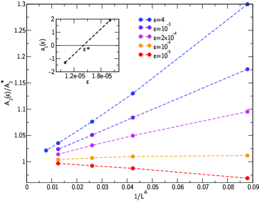V.3 Generalized Kremer-Grest model

The same analysis can be performed in the KG case. We first determine the optimal model, considering several values of $\epsilon_{nb}$ in the range $10^{-5}\leq\beta\epsilon_{nb}\leq 10^{-3}$ and values of $L$ in the range $100\leq L\leq 4000$. The results are reported in Table 6 and shown in Fig. 11. In the limit $L\to\infty$ all data converge to the same value, in agreement with universality. However, for finite $L$, deviations are typically large, except when $\beta\epsilon_{nb}$ is approximately $10^{-5}$. Repeating the analysis presented for the spherocylinder model, we obtain the optimal value, see Fig. 11,

$$\beta\epsilon_{nb}^{*}=1.41(6)\cdot 10^{-5},$$ (18)

where the error (in parentheses) takes also into account the uncertainties on $A_{2,GS}$, $\Delta$, and $\Delta_{2}$. It is interesting to compare this result with the one for the hard-sphere model using the Barker-Henderson mapping. As $\beta\epsilon_{nb}^{*}$ is very small, we can use the asymptotic behavior $d_{BH}/\sigma\approx(\beta\epsilon_{nb})^{1/12}\Gamma(11/12)\approx 1.056(\beta\epsilon_{nb})^{1/12}$ (see Appendix for the derivation). For the optimal model we obtain $d_{BH}\approx 0.416\sigma\approx 0.43b$, which is the value obtained above for the hard-sphere model.

The behavior of the generalized KG model for $\epsilon_{nb}<\epsilon_{nb}^{*}$ is again expected to be described by the TPM provided we define $z$ as $z=a_{KG}v(\epsilon_{nb})L^{1/2}$ with

$$v(\epsilon_{nb})={1\over 2\sigma^{3}}\int d^{3}r\,(1-e^{-\beta V_{LJ}(r,\epsilon_{nb})}).$$ (19)

Since we will be interested in values of $\epsilon_{nb}$ smaller than $\epsilon^{*}_{nb}$, we can replace the previous expression with its asymptotic behavior (see Appendix), $v(\epsilon_{nb})\approx(2\pi/3)(\beta\epsilon_{nb})^{1/4}\Gamma(3/4)\approx 2.567(\beta\epsilon_{nb})^{1/4}$. To compute $a_{KG}$, we take advantage of the Barker-Henderson mapping. Since we expect $z$ to be approximately equal to $a_{HS}v_{HS}(d_{BH}/b)L^{1/2}$, comparing the two expressions and using $b/\sigma\approx 0.97$, we obtain $a_{KG}\approx 0.70$. Therefore, we can simply define

$$z=1.80(\beta\epsilon_{nb})^{1/4}L^{1/2}.$$ (20)

To verify this prediction, we have performed simulations for $\beta\epsilon_{nb}=8\cdot 10^{-13}$. Using the TPM expression (5) we predict $A_{2}\approx 0.96$ for this value of the nonbonding parameter. Simulations for $L=1000$ give $A_{2}=0.992(3)$, in reasonable agreement.

VI Conclusions

One of the basic tenets of the theory of polymer solutions is the concept of universality deGennes-79 ; Freed-87 ; dCJ-book ; Schaefer-99 . The thermodynamic behavior and large-scale structure of these typical soft-matter systems can be described in a wide concentration range (the so-called dilute and semi-dilute regimes) by using a limited number of microscopic variables that depend on the specificities of the experimental system. Because of universality, theoretical predictions can be obtained by using simplified models, in which only a few of the properties of the original system are retained. Lattice self-avoiding walks have been extensively used and so have several continuum models, like the THSM and the KG model DH-86 ; DH-88 ; GK-86 . Although they all have the same behavior for long polymers, for chains of a few hundred monomers (this is the typical number in finite-density simulations) they give predictions that significantly differ from the asymptotic value. For instance, for $L=100$ the THSM and the KG model overestimate $A_{2}$ (or the equivalent interpenetration ratio $\Psi$) by 30%, while the self-avoiding walk is only slightly more accurate, with a discrepancy of 12%. Even worse, discrepancies increase as one enters the semidilute regime. For instance, if $Z=\beta P/\rho_{p}$ ($P$ is the pressure and $\rho_{p}$ the polymer number density) is the compressibility factor, JHGJM-12 reports $Z\approx 100$ for a polymer packing fraction $\phi_{p}=10$ if one uses the THSM with $L=100$. This is a factor of three larger than the result $Z\approx 34$ obtained by using an equation of state appropriate for very long good-solvent polymers Pelissetto-08 . It is therefore clear that in the semidilute region the THSM with such a number of monomers is far from the universality regime, and hence its predictions do not agree with what would be obtained in a different model or in an experimental system.

To overcome these problems, one can consider optimal models in which the approach to the universal limit is faster. The Domb-Joyce model DJ-72 is a simple generalization of the more common self-avoiding walk model, that allows one to obtain asymptotic results for small monomer numbers by appropriately choosing the value of the energy penalty BN-97 ; CMP-06 ; DP-16 ; Clisby-17 . There are, however, situations, in which a lattice model or a model in which self-intersections are allowed is not convenient. For instance, one cannot study solid phases (this is of interest for high-functionality star polymers star ) nor use it in all those contexts in which concatenation and topology are important.

In this paper we consider two continuum polymers models, which are simple generalizations of the THSM and of the KG model. By an appropriate choice of a single parameter, we obtain improved models which show a fast convergence. They can be conveniently used to study thermodynamics and phase diagrams, but, since in both cases bonds can cross, they are not appropriate for dynamical or topological studies. Thick self-avoiding chains, obtained by linking spherocylinders of length $b$ and diameter $d$, have none of these limitations. Bond intersections are strictly forbidden and there exists a value of the ratio $d/b$ ($d/b\approx 0.275$) for which the model is optimal. For $d/b>0.275$ corrections increase with $d/b$, so the largest $d/b$ is, the largest the number $L$ of monomers has to be in order to observe the universal asymptotic behavior. In the opposite regime we observe a crossover between ideal ($d/b\approx 0$) and good-solvent behavior, which can be described by using the two-parameter model Yamakawa-71 ; dCJ-book ; Schaefer-99 ; CMP-08 , which parametrizes the temperature dependence in the vicinity of the $\theta$ point.

It is important to stress that, although we have determined the optimal interaction by considering linear chains, the optimal models show a fast convergence to the asymptotic limit for any polymer topology. For instance, the optimal Domb-Joyce model determined by considering linear chains CMP-06 ; DP-16 ; Clisby-17 is also optimal when applied to star polymers, see the extensive analysis presented in RP-13 . Therefore, the results apply to any type of highly functionalized branched polymers. It is also interesting to investigate the behavior of cyclic chains. Renormalization-group arguments guarantee the optimality of the models as long as no constraint on the polymer topology is imposed, i.e., if one averages over all cyclic chains, independently of the knot type. If one considers instead polymers of fixed knot type, the behavior is less clear, as new corrections might appear. It must be noted, however, that all numerical simulations, see, e.g., BO-12 , indicate the presence of finite-size corrections decaying as $L^{-\Delta_{k}}$, with $\Delta_{k}\approx 0.5$ for all knot types. These results suggest that $\Delta_{k}$ coincides with the standard exponent $\Delta$, so that the corrections observed at fixed knot type are associated with the renormalization-group operator that controls the approach to the universal limit in any polymer model. If this is the case, the model with optimal interaction should be optimal also for chains of fixed knot type. This issue is presently under investigation.

Finally, it is tempting to use our results for thick self-avoiding chains to get some physical insight on the behavior of double-stranded DNA filaments. In particular, we can address the question under which conditions DNA can be considered as a model good-solvent polymer. The ratio $d/b$ can be effectively changed by varying the ionic strength $I$ of the solution. Using the results of Stigter-77 ; RCV-93 ; VC-95 and assuming that the effective diameter $d$ scales as $1/\sqrt{I}$, in analogy with the behavior of the Debye length that sets the scale for the electrostatic interactions, we obtain $d=d_{0}/\sqrt{I}$, where $d_{0}=1.6$-1.9 nm$\cdot$M^1/2 for a monovalent salt (Na⁺ for instance). For the Kuhn length $\ell_{K}$ several results are available in the literature, which all predict $\ell_{K}$ of the order of 100 nm for $I$ varying between 1 mM and 200 mM. We assume that our model provides a realistic description of DNA provided that $b$ is identified with $\ell_{K}$. Therefore, we predict that good-solvent behavior for relatively small values of $L$ should be observed for $d/\ell_{K}\approx 0.27$. Using the results reported above, we can correspondingly obtain the optimal ionic strengh: $I=3$-6 mM for a monovalent salt. The corresponding Kuhn length is $\ell_{K}=90$-110 nm, i.e., approximately 300 base pairs. Therefore, for values of $I$ in the optimal range, one should be able to observe good-solvent behavior by using DNA of 30000 base pairs.

The optimal value of $I$ is, however, well below physiological conditions ($I\sim 100$-200 mM). If we take $I=150$ mM, we predict $d/\ell_{K}\approx 0.05$. Also in this regime we can predict theoretically the observed behavior, as long as the DNA filaments are significantly longer than the Kuhn length. We can indeed use the wealth of results available for the TPM Yamakawa-71 ; Schaefer-99 ; dCJ-book ; CMP-08 ; DPP-13-Thermal . The only external input is the model-dependent constant $a$ entering the definition of the TPM variable $z$. If we assume that our model provides a reasonable description of DNA, we predict $z\approx z_{0}L^{1/2}$, where $z_{0}\approx 0.03$-0.04, and $L$ is the ratio between the length of the filament and the Kuhn length. Note that, for such small values of $d/b$, scaling corrections are large (see Fig. 2 for instance) and good-solvent behavior may be unattainable in practice, in agreement with the conclusions of TMDD-13 . Indeed, as good-solvent behavior is (very roughly) observed for $z\mathrel{\hbox to0.0pt{\lower 3.0pt\hbox{$\mathchar 536\relax$}\hss}\raise 2.0pt\hbox{$\mathchar 318\relax$}}5$ (see the supplementary material of DPP-14-GFVT ), DNA is close to the universal asymptotic regime only for $L\mathrel{\hbox to0.0pt{\lower 3.0pt\hbox{$\mathchar 536\relax$}\hss}\raise 2.0pt\hbox{$\mathchar 318\relax$}}20000$-30000, i.e., when the filament has at least $10^{6}$ base pairs.

G.D. thanks C. Micheletti and C. Pierleoni for fruitful discussions.

Appendix A Computation of integrals for the generalized Kremer-Grest model

In Section V.3 we use the asymptotic expansion of some integrals involving the Kremer-Grest potential. The general integral we consider is

$$I(s,\alpha)=\int_{0}^{a}dx\ x^{s}\left\{1-\exp\left[-\alpha\left({1\over x^{12}}-{1\over x^{6}}+b\right)\right]\right\},$$ (21)

where $-1<s<5$, $a$ is a positive finite number and $b$ is a second constant. We wish to compute the expansion of this integral for $\alpha\to 0$. First, we rewrite the integral as

$$I(s,\alpha) = (1-e^{-b\alpha})\int_{0}^{a}dx\ x^{s}$$ (22)

$$- e^{-b\alpha}\int_{a}^{\infty}dx\ x^{s}\left(1-e^{-\alpha/x^{12}+\alpha/x^{6}}\right)$$

$$+ e^{-b\alpha}\int_{0}^{\infty}dx\ x^{s}\left(1-e^{-\alpha/x^{12}+\alpha/x^{6}}\right).$$

The first term is obviously of order $\alpha$. In the second term, for $s<5$ we can expand the exponential to first order in $\alpha$, proving that this contribution is of order $\alpha$, too. Therefore, we obtain

$$I(s,\alpha)=\int_{0}^{\infty}dx\ x^{s}\left(1-e^{-\alpha/x^{12}+\alpha/x^{6}}\right)+O(\alpha).$$ (23)

Now, we change variable, defining $y=\alpha/x^{12}$. We obtain

$$I(s,\alpha)\approx{\alpha^{(s+1)/12}\over 12}\int_{0}^{\infty}dy\ y^{-(s+13)/12}(1-e^{-y+\sqrt{\alpha y}})$$

$$\quad\approx{\alpha^{(s+1)/12}\over 12}\int_{0}^{\infty}dy\ y^{-(s+13)/12}(1-e^{-y})$$

$$\quad=-{\alpha^{(s+1)/12}\over 12}\Gamma\left(-{1+s\over 12}\right)$$

$$\quad={\alpha^{(s+1)/12}\over s+1}\Gamma\left({11-s\over 12}\right)+O(\alpha^{(s+7)/12}),$$ (24)

where, in the last line, we have explicitly reported the order of the neglected terms.

References

- (1) Binder K (ed.) 1996 Monte Carlo and Molecular Dynamics Simulations in Polymer Science (Oxford, UK: Oxford University Press)
- (2) de Gennes P G 1979 Scaling Concepts in Polymer Physics (Ithaca, NY: Cornell University Press)
- (3) Freed K F 1987 Renormalization Group Theory of Macromolecules (New York: Wiley)
- (4) Doi M and Edwards S F 1988 The Theory of Polymer Dynamics (Oxford: Clarendon Press)
- (5) des Cloizeaux J and Jannink G 1990 Polymers in Solution: Their Modelling and Structure (Oxford: Clarendon Press)
- (6) Schäfer L 1999 Excluded Volume Effects in Polymer Solutions (Berlin: Springer).
- (7) Valle F, Favre M, De Los Rios P, Rosa A and Dietler G 2005 Scaling exponents and probability distributions of DNA end-to-end distance Phys. Rev. Lett. 95 158105
- (8) Nepal M, Yaniv A, Shafran E and Krichevsky O 2013 Structure of DNA coils in dilute and semidilute solutions, Phys. Rev. Lett. 110 058102
- (9) Tree D R, Muralidhar A, Doyle P S and Dorfman K D 2013 Is DNA a good model polymer? Macromolecules 46 8369
- (10) Dickman R and Hall C K 1986 Equation of state for chain molecules: Continuous-space analog of Flory theory J. Chem. Phys. 85 4108
- (11) Dickman R and Hall C K 1988 High-density Monte Carlo simulations of chain molecules: Bulk equation of state and density profile near walls J. Chem. Phys. 89 3168
- (12) Grest G S and Kremer K 1986 Molecular dynamics simulation for polymers in the presence of a heat bath Phys. Rev. A 33 3628
- (13) de Gennes P G 1972 Exponents for the excluded volume problem as derived by the Wilson method Phys. Lett. A 38 339
- (14) Wegner F J 1976 The Critical State, General Aspects Phase Transitions and Critical Phenomena Domb C and Green M S (eds) vol 6 (New York: Academic Press)
- (15) Privman V, Hohenberg P C and Aharony A 1991 Universal Critical-Point Amplitude Relations Phase Transitions and Critical Phenomena Domb C and Lebowitz J (eds) vol 14 (London: Academic Press)
- (16) Pelissetto A and Vicari E 2002 Critical phenomena and renormalization-group theory Phys. Rep. 368 549
- (17) Oono Y 1985 Statistical physics of polymer solutions: Conformation-space renormalization-group approach Adv. Chem. Phys. 61 301 (Sec. V)
- (18) Wang S Q, Douglas J F and Freed K F 1986 Corrections to preaveraging approximation within the Kirkwood-Riseman model for flexible polymers: Calculations to second order in with both hydrodynamic and excluded volume interactions J. Chem. Phys. 85 3674
- (19) Wang S Q and Freed K F 1986 Renormalization group study of Rouse-Zimm model of polymer dynamics through second order in J. Chem. Phys. 85 6210
- (20) Schaub B, Friedman B A and Oono Y 1985 Time-dependent correlations of a self-avoiding polymer chain Phys. Lett. A 110 136
- (21) Stepanow S and Helmis G 1989 Renormalization-group study of the dynamical viscosity of dilute solutions of self-avoiding polymer chains Phys. Rev. A 39 6037
- (22) Grassberger P 1997 Pruned-enriched Rosenbluth method: Simulations of theta polymers of chain length up to 1,000,000 Phys. Rev. E 56 3682
- (23) Clisby N 2010 Efficient implementation of the pivot algorithm for self-avoiding walks J. Stat. Phys. 140 349
- (24) Belohorec P and Nickel B G 1997 Accurate universal and two-parameter model results from a monte-carlo renormalization group study Guelph University report (unpublished) Belohorec P 1997 Renormalization group calculation of the universal critical exponents of a polymer molecule Guelph University PhD thesis (available at www.collectionscanada.gc.ca/obj/s4/f2/dsk3/ftp04/nq24397.pdf).
- (25) Lue L and Kiselev S B 1999 Crossover approach to scaling behavior in dilute polymer solutions: Theory and simulation J. Chem. Phys. 110 2684 Lue L and Kiselev S B 2001 Crossover behavior of star polymers in good solvents J. Chem. Phys. 114 5026
- (26) Caracciolo S, Mognetti B M and Pelissetto A 2006 Virial coefficients and osmotic pressure in polymer solutions in good-solvent conditions, J. Chem. Phys. 125 094903
- (27) D’Adamo G and Pelissetto A 2016 Improved model for mixtures of polymers and hard spheres J. Phys. A: Math Theor. 49 504006
- (28) Clisby N 2017 High resolution Monte Carlo study of the Domb-Joyce model arXiv:1705.01249 [cond-mat.stat-mech]
- (29) Bolhuis P G, Louis A A, Hansen J P and Meijer E J 2001 Accurate effective pair potentials for polymer solutions J. Chem. Phys. 114 4296
- (30) Müller-Plathe F 2002 Coarse-graining in polymer simulation: From the atomistic to the mesoscopic scale and back Chem. Phys. Chem. 3 754
- (31) Pierleoni C, Capone B and Hansen J P 2007 A soft effective segment representation of semidilute polymer solutions J. Chem. Phys. 127 171102
- (32) Peter C and Kremer K 2009 Multiscale simulation of soft matter systems — from the atomistic to the coarse-grained level and back Soft Matter 5 4357
- (33) D’Adamo G, Pelissetto A and Pierleoni C 2012 Coarse-graining strategies for polymer solutions Soft Matter 8 5151
- (34) D’Adamo G, Pelissetto A and Pierleoni C 2012 Consistent and transferable coarse-grained model for semidilute polymer solutions in good solvent J. Chem. Phys. 137 024901
- (35) Karimi-Varzaneh H A and Müller-Plathe F 2012 Coarse-grained modeling for macromolecular chemistry Multiscale Molecular Methods in Applied Chemistry, Kirchner B and Vrabec J (eds) Top. Curr. Chem. 307 (Berlin:Springer) 295-321
- (36) Noid W G 2013 Systematic methods for structurally consistent coarse-grained models, Methods Mol. Biol. 924 487Noid W G 2013 Perspective: Coarse-grained models for biomolecular systems J. Chem. Phys. 139 090901
- (37) Padding J T and Briels W J 2001 Uncrossability constraints in mesoscopic polymer melt simulations: Non-Rouse behavior of C120H242 J. Chem. Phys. 115 2846
- (38) Orlandini E and Whittington S G 2007 Statistical topology of closed curves: Some applications in polymer physics Rev. Mod. Phys. 79 611-642
- (39) Forgan R S, Sauvage J P and Stoddard J F 2011 Chemical Topology: Complex Molecular Knots, Links, and Entanglements Chem. Rev. 111 5434-5464
- (40) Janse van Rensburg E J, Sumners D A W, Wassermann E and Whittington S G 1992 Entanglement complexity of self-avoiding walks J. Phys. A: Math. Gen. 25 6557-6566
- (41) Tubiana L, Rosa A, Fragiacomo F and Micheletti C 2013 Spontaneous Knotting and Unknotting of Flexible Linear Polymers: Equilibrium and Kinetic Aspects Macromolecules 46 3669-3678
- (42) Evans N H and Beer P D 2014 Review Article: Progress in the synthesis and exploitation of catenanes since the Millennium Chem. Soc. Rev. 43 4658-4683
- (43) Wassermann S A and Cozzarelli N R 1986 Biochemical topology: Applications to DNA recombination and replication Science 232 951-960
- (44) Vologodskii A and Rybenkov V V 2009 Perspective: Simulation of DNA catenanes Phys. Chem. Chem Phys. 11 10543-10552
- (45) Aharony A and Ahlers G 1980 Universal ratios among correction-to-scaling amplitudes and effective critical exponents Phys. Rev. Lett. 44 782
- (46) Janse van Rensburg E J, Whittington S G and Madras N 1990 The pivot algorithm and polygons: results on the FCC lattice J. Phys. A: Math. Gen. 23 1589
- (47) Fuereder I and Zifferer G 2011 Monte Carlo simulation studies of ring polymers at athermal and theta conditions J. Chem. Phys. 135 184906
- (48) Hsu H-P, Nadler W and Grassberger P 2004 Scaling of star polymers with 1–80 arms Macromolecules 37 4658
- (49) Randisi F and Pelissetto A 2013 High-functionality star-branched macromolecules: Polymer size and virial coefficients J. Chem. Phys. 139 154902
- (50) Clisby N 2010 Accurate estimate of the critical exponent for self-avoiding walks via a fast implementation of the pivot algorithm Phys. Rev. Lett. 104 055702
- (51) Vologodskii A V, Levene S D, Klenin K V, Frank-Kamenetskii M D and Cozzarelli N R 1992 Conformational and Thermodynamic Properties of Supercoiled DNA J. Mol. Biol. 227 1224
- (52) Rybenkov V V, Cozzarelli N R and Vologodskii A V 1993 Probability of DNA knotting and the effective diameter of the DNA double helix, Proc. Natl. Acad. Sci. (USA) 90 5307-5311
- (53) Vologodskii A and Cozzarelli N R 1995 Modeling of long-range electrostatic interactions in DNA Biopolymers 35 289-296
- (54) Gonzalez O and Maddocks J H 1999 Global curvature, thickness, and the ideal shapes of knots Proc. Natl. Acad. Sci. (USA) 96 4769
- (55) Stasiak A and Maddocks J H 2000 Best packing in proteins and DNA Nature 406 251
- (56) Millet K C, Piatek M and Rawdon E 2008 Polygonal knot space near ropelength-minimized knots J. Knot Theory Ramifications 17 601-631
- (57) Uehara E and Deguchi T 2015 Characteristic length of the knotting probability revisited J. Phys.: Condens. Matter 27 354104 Uehara E and Deguchi T, Knotting probability and the scaling behavior of self-avoiding polygons under a topological constraint arXiv:1704.07510
- (58) Plunkett Zirbel L and Chapman K 2016 Off-lattice random walks with excluded volume: a new method of generation, proof of ergodicity and numerical results J. Phys. A: Math. Theor. 49 135203
- (59) Vega C and Lago S 1994 A fast algorithm to evaluate the shortest distance between rods Computers Chem. 18 55-59
- (60) Rubinstein M and Colby R H C 2003 Polymer Physics (Oxford: Oxford University Press)
- (61) Zimm B H, Stockmayer W H and Fixman M 1953 Excluded Volume in Polymer Chains J. Chem. Phys. 21 1716
- (62) Yamakawa H 1971 Modern Theory of Polymer Solutions (New York: Harper–Row)
- (63) Caracciolo S, Mognetti B M and Pelissetto A 2008 Two-parameter model predictions and -point crossover for linear-polymer solutions J. Chem. Phys. 128 065104
- (64) D’Adamo G, Pelissetto A and Pierleoni C 2013 Consistent coarse-graining strategy for polymer solutions in the thermal crossover from good to solvent J. Chem. Phys. 139 034901
- (65) Madras N and Sokal A D 1988 The pivot algorithm: A highly efficient Monte Carlo method for the self-avoiding walk J. Stat. Phys. 50 109
- (66) Kennedy T 2002 A faster implementation of the pivot algorithm for self-avoiding walks J. Stat. Phys. 106 407
- (67) Berry G C 1966 Thermodynamic and Conformational Properties of Polystyrene. I. Light-Scattering Studies on Dilute Solutions of Linear Polystyrenes J. Chem. Phys. 44 4550
- (68) D’Adamo G, Pelissetto A and Pierleoni C 2014 Phase diagram of mixtures of colloids and polymers in the thermal crossover from good to solvent J. Chem. Phys. 141 024902
- (69) Pelissetto A and Hansen J-P 2005 Corrections to scaling and crossover from good- to -solvent regimes of interacting polymers J. Chem. Phys. 122 134904
- (70) Krüger B and Schäfer L 1994 Long polymer chains in good solvent: beyond the universal limit J. Phys. I (France) 4 757
- (71) Hall C K 1980 Polymer scaling theories for general interaction potentials J. Chem. Phys. 73 1446
- (72) Isihara A 1950 Determination of molecular shape by osmotic measurement J. Chem. Phys. 18 1446
- (73) Isihara A and Hayashida T 1951 Theory of high polymer solution. I. Second virial coefficient for rigid ovaloids models J. Phys. Soc. Jpn. 6 40-45
- (74) Kihara T 1953 Virial coefficients and models of molecules in gases Rev. Mod. Phys. 25 831
- (75) Domb C and Joyce G S 1972 Cluster expansion for a polymer chain J. Phys. C 5 956-976
- (76) Bolhuis P G, Louis A A and Hansen J P 2001 Many-body interactions and correlations in coarse-grained descriptions of polymer solutions Phys. Rev. E 64 021801
- (77) D’Adamo G, Pelissetto A and Pierleoni C 2012 Polymers as compressible soft spheres J. Chem. Phys. 136 224905
- (78) Causo M S 2002 Universal shape ratios for polymers grafted at a flat surface J. Chem. Phys. 117 6789
- (79) Sciutto S J 1996 The shape of self-avoiding walks J. Phys. A: Math. Gen. 29 5455
- (80) Zifferer G 1999 Monte Carlo simulation studies of the size and shape of linear and star-branched polymers embedded in the tetrahedral lattice Macromol. Theory Simul. 8 433 Zifferer G and Preusser W 2001 Monte Carlo simulation studies of the size and shape of ring polymers Macromol. Theory Simul. 10 397
- (81) Škrbić T, Hoang T X and Giacometti A 2016 Effective stiffness and formation of secondary structures in a protein-like model J. Chem. Phys. 145 084904
- (82) Barker J A and Henderson D 1967 Perturbation theory and equation of state for fluids: The square-well potential J. Chem. Phys. 47 2856 Barker J A and Henderson D 1967 Perturbation theory and equation of state for fluids. II. A successful theory of liquids J. Chem. Phys. 47 4714
- (83) Jover J, Haslam A J, Galindo A, Jackson G and Müller E A 2012 Pseudo hard-sphere potential for use in continuous molecular-dynamics simulation of spherical and chain molecules J. Chem. Phys. 137 144505
- (84) Pelissetto A 2008 Osmotic pressure and polymer size in semidilute polymer solutions under good-solvent conditions J. Chem. Phys. 129 044901
- (85) Likos C N, Löwen H, Watzlawek M, Abbas B, Jucknischke O, Allgaier J and Richter D 1998 Star polymers viewed as ultrasoft colloidal particles Phys. Rev. Lett. 80 4450Watzlawek M, Likos C N and Löwen H 1999 Phase diagram of star polymer solutions Phys. Rev. Lett. 82 5289Laurati M, Stellbrink J, Lund R, Willner L, Richter D and Zaccarelli E 2005 Starlike micelles with starlike interactions: A quantitative evaluation of structure factors and phase diagram Phys. Rev. Lett. 94 195504Menichetti R, Pelissetto A and Randisi F 2017 Thermodynamics of star polymer solutions: A coarse-grained study J. Chem. Phys. 146 244908
- (86) Baiesi M and Orlandini E 2012 Universal properties of knotted polymer rings Phys. Rev. E 86 031805
- (87) Stigter D 1977 Interactions of highly charged colloidal cylinders with applications to double-stranded DNA Biopolymers 16 1435
- (88) Dobrynin A V and Carrillo J-M Y 2009 Swelling of biological and semiflexible polyelectrolytes J. Phys. Condens. Matter 21 424112
- (89) Brunet A, Tardin C, Salomé L, Rousseau P, Destainville N and Manghi M 2015 Macromolecules 48 3641