Continuous-Variable Sampling from Photon-Added or Photon-Subtracted Squeezed States

Abstract

We introduce a new family of quantum circuits in continuous variables and we show that, relying on the widely accepted conjecture that the polynomial hierarchy of complexity classes does not collapse, their output probability distribution cannot be efficiently simulated by a classical computer. These circuits are composed of input photon-subtracted (or photon-added) squeezed states, passive linear optics evolution, and eight-port homodyne detection. We address the proof of hardness for the exact probability distribution of these quantum circuits by exploiting mappings onto different architectures of sub-universal quantum computers. We obtain both a worst-case and an average-case hardness result. Hardness of Boson Sampling with eight-port homodyne detection is obtained as the zero squeezing limit of our model. We conclude with a discussion on the relevance and interest of the present model in connection to experimental applications and classical simulations.

I Introduction

In the recent years we have witnessed an increasing interest in quantum circuits that define sub-universal models of quantum computation Aaronson and Arkhipov (2013); Bremner et al. (2010, 2016); Farhi and Harrow (2016); Morimae et al. (2014). These models lie somewhere in-between classical and universal quantum computing, in the sense that, although not possessing the full computational power of a universal quantum computer, they allow for the outperformance of classical computational capabilities with respect to specific problems. Beyond their conceptual relevance, the reason for this interest is that these models require less experimental resources than universal quantum computers do. Therefore, they may allow next future experimental demonstration of quantum advantage, i.e. the predicted speed-up of quantum devices over classical ones for some computational tasks.

These models are often associated with sampling problems for which the task is to draw random numbers according to a specific probability distribution. Some of these probability distributions are likely to be hard to sample for classical computers, assuming widely accepted conjectures in computer science, for example with the celebrated Boson Sampling Aaronson and Arkhipov (2013).

In parallel, Continuous-Variable (CV) systems are being recognized as a promising alternative to the use of qubits, as they allow for the deterministic generation of unprecedented large quantum states, of up to one-million elementary systems Yokoyama et al. (2013); Yoshikawa et al. (2016), and also offer detection techniques, such as homodyne, with high efficiency and reliability.

Any given CV quantum circuit is defined by (i) a specific input state, (ii) a unitary evolution and (iii) measurements. An important theorem Bartlett et al. (2002); Mari and Eisert (2012) states that if all these elements are described by positive Wigner functions, then there exists a classical algorithm able to efficiently simulate this circuit. Hence, including a negative Wigner function element is mandatory in order to design a CV sub-universal quantum circuit that cannot be efficiently simulated by a classical device. By virtue of the Hudson theorem Soto and Claverie (1983), this necessarily corresponds to the use of non-Gaussian resources.

Therefore, if one aims at minimal extensions of Gaussian models, three different families of non trivial sub-universal quantum circuits can be defined, depending on whether the element yielding the Wigner function negativity is provided by the input state, the unitary evolution, or the measurement. Although Wigner negativity allows stepping outside the range of applicability of the theorem in Ref. Mari and Eisert (2012), it is by itself not sufficient to imply classical hardness Rahimi-Keshari et al. (2016). The classical hardness of circuits of the latter kind, corresponding to Gaussian Boson Sampling (GBS), was proven in Ref. Lund et al. (2014); Hamilton et al. (2016). These circuits are composed of input squeezed states, passive linear optics evolution, and photon counters. Circuits of the second kind are for instance related to the CV implementation of Instantaneous Quantum Computing – another sub-universal model, where input states and measurements are Gaussian, while the evolution contains non-Gaussian gates Douce et al. (2017); Douce et al (2017). First definitions of the former class of CV circuits, i.e. that display non-Gaussian input state and Gaussian operations and measurements, have been very recently considered Chakhmakhchyan and Cerf (2017); Lund et al. (2017). However, the measurement considered in Lund et al. (2017) is effectively a non-Gaussian measurement . Furthermore, the non-Gaussian input state considered in both references is a collection of single photons, that is still reminiscent of the standard Boson Sampling approach .

In this work, we define a new family of quantum circuits that take non-Gaussian input states and use Gaussian evolution and measurement. The circuits family that we consider has a further “CV flavor” with respect to Refs. Chakhmakhchyan and Cerf (2017); Lund et al. (2017), in that the non-Gaussian input states are single photon-subtracted (or single photon-added) squeezed states, and the measurement is Gaussian, namely eight-port homodyne detection Leonhardt (2010) . This model therefore is analog to the Photon-Added or photon-Subtracted Squeezed Vacuum (PASSV) sampling model of Ref. Olson et al. (2015) but with eight-port homodyne detection replacing photon counting. For this reason, we may refer to our model as to PASSV with CV Sampling. For brevity, however, we will use the acronym CVS in the remainder of our paper. This architecture is inspired by recent experiments performed at Laboratoire Kastler Brossel (LKB), where mode-selective single photon subtraction from a collection of multi-mode squeezed states has been recently demonstrated Ra et al. (2017), and where simultaneous detection of all the optical modes can also be implemented by means of multi-pixel homodyne detection Beck (2000); Ferrini et al. (2013).

Importantly, in contrast to Refs. Chakhmakhchyan and Cerf (2017); Lund et al. (2017), we are able to construct our proof as an “average-case” statement: we show that if two conjectures hold true then the underlying problem is hard with high probability. More specifically, we exhibit a construction that allows one to draw at random hard to sample circuits with high probability.

In Sec. II we define the model we are interested in, focusing on photon subtraction at the input, and in Sec. III we outline the proof of hardness of the corresponding output probability distribution, detailing the mappings needed to establish it. We give the detail of this proof in Sec. IV. In Sec. V we show that the proof can be easily extended to the case of input photon-added squeezed states, and we discuss other relevant extensions, such as the zero squeezing limit, and the choice of the measurement quadrature. Sec. VI is dedicated to discussing possible experimental implementations of our model. Conclusions and perspectives are presented in Sec. VII.

II Definition of the circuit family

Figure 1: A representation of a CVS circuit. In input are vacuum squeezed states and photon-subtracted vacuum squeezed states. The passive linear optics evolution is associated with the unitary matrix $Q$ defined in Eq.(1). Measurement is performed by eight-port homodyne detection.

CVS circuits, for which classical hardness will be proven in this paper, are defined as follows. Let $M$ be the total number of optical modes. We define the squeezing operator with squeezing parameter $s$ as $\hat{S}(s)=e^{-\frac{i}{2}(\ln{s})(\hat{q}\hat{p}+\hat{p}\hat{q})}$. The input is made of vacuum squeezed states $\ket{s}\equiv\hat{S}(s)\ket{0}$, and the squeezing is uniform over all the modes. We adopt the convention $[\hat{q},\hat{p}]=i$ for the quadratures commutation relation, i.e. $\Delta_{0}=1/2$ for the vacuum fluctuations. Given the corresponding action on the quadratures $\begin{pmatrix}\hat{q}\\ \hat{p}\end{pmatrix}\rightarrow\begin{pmatrix}s&0\\ 0&1/s\end{pmatrix}\begin{pmatrix}\hat{q}\\ \hat{p}\end{pmatrix},$ $s>1$ results in $p$-squeezing while $s<1$ in $q$-squeezing.

The first $m$ modes are single photon-subtracted squeezed states denoted by $\hat{a}\ket{s}$. The remaining $M-m$ modes are just squeezed states $\ket{s}$. We assume that the squeezing parameter $s$ is constant and does not depend on the number of modes $m$. We require that $m$ is even and that $M\geq 2m$.

The input modes undergo a passive linear evolution that is described by the unitary matrix $Q$ that belongs to the set of matrices of the form

$$Q=\Theta e^{-i\phi\Sigma}$$ (1)

with $\phi\in\mathbb{R},\Theta\in\mathcal{O}(M)$ and $\Sigma\in\mathcal{O}_{S}(M)$, i.e., $\Theta$ is a real orthogonal matrix and $\Sigma$ is a real symmetric orthogonal matrix, and hence satisfies $\Sigma^{2}=1$. This choice of matrices will allow us to derive a convenient expression for the output probability distribution of CVS circuits in Sec. IV.

Finally, the mode quadratures are measured by eight-port homodyne detection, i.e. by projecting the output states onto displaced squeezed states $\ket{\alpha_{i},r}=\hat{D}(\alpha_{i})\hat{S}(r)\ket{0}$. The arbitrary parameter $r>0$ is constant with the number of modes and $\alpha_{i}=\sqrt{(1+r^{2})/2}(q_{i}+ip_{i}/r)$ corresponds to the displacement value of the $i^{th}$ mode. $q_{i}$ and $p_{i}$ are the measured outcomes at the (distinct) output modes of the eight-port homodyne detector. $\hat{D}(\alpha)$ is the displacement operator $\hat{D}(\alpha)=e^{\alpha\hat{a}^{\dagger}-\alpha^{*}\hat{a}}$. This modelization is presented in detail in Appendix A (see also Ref.Leonhardt (2010)) . The limit of perfect or zero reflectivity (corresponding to projection onto infinitely squeezed states) yields back the case of standard homodyne detection. As already considered in Refs. Douce et al. (2017); Chakhmakhchyan and Cerf (2017), in order to give meaning to the obtained probability distribution, that must be defined on discrete values, we assume a finite binning of size $\eta$ for the output probability density of CVS circuits Paris et al. (2003). This allows for the definition of a set of indices $\bar{b}=(b^{(q)}_{1},\ldots,b^{(q)}_{M},b^{(p)}_{1},\ldots,b^{(p)}_{M})$ that corresponds to bins for the ${q}$ and ${p}$ quadratures. We denote $\text{Pr}_{\rm CVS}^{\eta}(\bar{b}|\bar{n})$ as the discrete probability that the $i^{th}$-mode measurement outcome $(x_{i},x_{i+M})=(q_{i},p_{i})$ falls into the boxes $(B^{(q)}_{i},B^{(p)}_{i})=[({b}^{(q)}_{i}-\frac{1}{2})\eta,(b^{(q)}_{i}+\frac{1}{2})\eta],[({b}^{(p)}_{i}-\frac{1}{2})\eta,(b^{(p)}_{i}+\frac{1}{2})\eta]$ for all $i\in\{1,\ldots,M\}$, given the input $\bar{n}=(n_{1},\ldots,n_{M})\in\{0,1\}^{M}$, where the ones correspond to photon-subtracted squeezed states and the zeros to squeezed states. Note that this probability distribution is related to the real-valued probability density associated with CVS circuits, $\text{Pr}_{\text{CVS}}(\bar{x}|\bar{n})$, by

$$\text{Pr}^{\eta}_{\text{CVS}}(\bar{b}|\bar{n})\equiv\prod_{i=1}^{M}{\left[\int_{B^{(q)}_{i}}\int_{B^{(p)}_{i}}{\mathrm{d}{q}_{i}\mathrm{d}{p}_{i}\text{Pr}_{\text{CVS}}(\bar{x}|\bar{n})}\right]}$$ (2)

where $\bar{x}=(x_{1},\ldots,x_{2M})=(q_{1},\dots,q_{M},p_{1},\dots,p_{M})$ is the continuously distributed measurement outcome. This model of detection is equivalent to perfect eight-port homodyne detection, followed by a binning of the outcome results performed at the stage of post-processing. We assume a scaling of the window size $\eta$ with the number of modes, namely $\eta=2^{-poly(M)}$, analogous to what has been done in Ref. Chakhmakhchyan and Cerf (2017).

Our aim is to prove that the probability distribution $\text{Pr}^{\eta}_{\text{CVS}}(\bar{b}|\bar{m})$, where $\bar{m}=(1,\ldots,1,0,\ldots,0)$ describes the input photon subtractions, is hard to sample for a classical computer, both in the worst case scenario and in the average case scenario. In the next section we outline the proof.

III Auxiliary models and structure of the proof of hardness

Figure 2: An alternative representation of a CVS circuit. The input has been rewritten using the mapping of single photon subtraction onto squeezing applied to single photons. $S(s)$ is the unitary associated to a squeezing with parameter $s$, while $Q$ is a passive linear optics transformation. The output is measured using eight-port homodyne detection.

In order to prove the hardness of the model that we are interested in, we define auxiliary computational models that we address as intermediate steps. First, we note that the input photon-subtracted squeezed states can be mapped onto single photon states, followed by squeezing. Indeed the squeezing operator $\hat{S}(s)$ satisfies $\hat{S}^{{\dagger}}(s)\hat{a}\hat{S}(s)=c_{s}\hat{a}-s_{s}\hat{a}^{\dagger}$ with $c_{s}=\cosh(\ln s)$ and $s_{s}=\sinh(\ln s)$. Therefore we obtain

$$\hat{a}\ket{s}=c_{s}\hat{S}(s)\hat{a}\ket{0}-s_{s}\hat{S}(s)\hat{a}^{{\dagger}}\ket{0}=-s_{s}\hat{S}(s)\ket{1},$$ (3)

where the factor $s_{s}$ stems from the normalization of the left hand side of Eq.(3). As a consequence, the circuit represented in Fig.1 is fully equivalent to a circuit with input single photon states in correspondence with the photon-subtractions, followed by a squeezing operator $\hat{S}(s)$ applied to all the modes (Fig.2). By virtue of the identity in Eq.(3), the two architectures share the same probability distribution of the measurement outcomes $\text{Pr}^{\eta}_{\text{CVS}}(\bar{b}|\bar{m})$ in Eq.(2), and therefore we refer to both configurations by CVS.

Next, we use time-reversal, i.e. the symmetry of Born’s rule, in order to relate the probability distribution of CVS circuits to a matrix permanent. Because of the symmetry of Born’s rule, the role of measurements and input states can be interchanged, while the probability distribution remains identical: input single photon states correspond to detection of single photons in the output modes and eight-port homodyne detection corresponds to input squeezed states, with a squeezing parameter $k\equiv 1/r$. The unitary evolution in between the input state and the output measurement is conjugated. Therefore, in the time-reversed version of the circuit in Fig.(2), squeezing occurs in the opposite quadrature, i.e. with parameter $l\equiv 1/s$, and is preceded by the passive linear optics evolution $T=Q^{\dagger}$.

We define this model as “Time-Reversed-Continuous-Variable Sampling” (TR-CVS). Its structure is outlined in Fig. 3. By virtue of the symmetry of Born’s rule,

$$\text{Pr}_{\text{CVS}}(0,\ldots,0|\bar{m})=\text{Pr}_{\text{TR-CVS}}(\bar{m})$$ (4)

where $\text{Pr}_{\text{TR-CVS}}(\bar{m})$ is the probability of detecting the output pattern $\bar{m}$ in the TR-CVS circuit, and corresponds in the original circuit to the presence of $m$ single-photons (in turn related to single photon-subtractions in the original CVS model), while $\text{Pr}_{\text{CVS}}(0,\ldots,0|\bar{m})$ is the probability density function of the corresponding CVS circuit, evaluated at $(0,\ldots,0)$. This allows us to establish a link between the output probability distribution of TR-CVS circuits and a matrix permanent.

Figure 3: A representation of a TR-CVS circuit. The unitary matrix $T=Q^{\dagger}$ corresponds to a passive linear optics evolution, $Q$ as defined in Eq.(1), while $S(l)$ and $S(k)$ are the unitary matrices associated to the squeezing transformations with parameters $l=1/s$ and $k=1/r$ respectively.

The proof of classical hardness for the probability distribution $\text{Pr}^{\eta}_{\text{CVS}}(\bar{b}|\bar{m})$ in Eq.(2), then, is structured according to the following steps, that retrace the mappings outlined above:

1. We relate the probability distribution of TR-CVS circuits to a matrix hafnian. We then use time reversal symmetry Eq.(4) to connect the probability distribution of TR-CVS circuits to the value $\text{Pr}_{\text{CVS}}(0,\ldots,0|\bar{m})$ of the probability density of CVS circuits. In addition to the properties of the matrix $\Sigma$ in Eq.(1), and to the relation between hafnian and permanent, it yields that approximating multiplicatively $\text{Pr}_{\text{CVS}}(0,\ldots,0|\bar{m})$ is #P-hard (Theorem 1).

2. We then show that sampling from $\text{Pr}^{\eta}_{\text{CVS}}(\bar{b}|\bar{m})$ allows for a multiplicative approximation of $\text{Pr}_{\text{CVS}}(0,\ldots,0|\bar{m})$ in the third level of the polynomial hierarchy. This will require making use of a Taylor expansion of the probability $\text{Pr}^{\eta}_{\text{CVS}}(\bar{b}|\bar{m})$, around $\bar{b}_{0}=(0,\ldots,0)$, for small $\eta$, as well as invoking the Stockmeyer’s counting algorithm. Together with the previous point and standard complexity theory arguments – see, e.g. Aaronson and Arkhipov (2013); Bremner et al. (2016), this allows us to claim the hardness of the original model in Fig. 1. The claim can then be made as an average statement (Theorem 2) using two conjectures.

IV Proof of Hardness for CVS circuits

We now explain in detail the proof of hardness sketched in the previous section. Let us first introduce our notations.

Any $M$-mode Gaussian state can be described by a $2M\times 2M$ covariance matrix $\sigma$ whose coefficients are defined for $k,l\in\{1,\ldots,2M\}$ by $\sigma_{kl}=\frac{1}{2}\left<\left\{R_{k}R_{l}\right\}\right>-\left<R_{k}\right>\left<R_{l}\right>$ where $\vec{R}=({\hat{q}}_{1},\ldots,\hat{q}_{M},\hat{p}_{1},\ldots,\hat{p}_{M})$  Dutta et al. (1995). Alternatively and more conveniently, one can describe covariance matrices and evolutions in the complex basis $\vec{\Gamma}={(\hat{a}}_{1},\ldots,{\hat{a}}_{M}{,\hat{a}}_{1}^{{\dagger}}{,\ldots,\hat{a}}_{M}^{{\dagger}})$, where ${\hat{a}}_{j}=\frac{1}{\sqrt{2}}({\hat{q}}_{j}+i{\hat{p}}_{j})$ and ${\hat{a}}_{j}^{{\dagger}}=\frac{1}{\sqrt{2}}({\hat{q}}_{j}-i{\hat{p}}_{j})$ for all $j\in\{1,\ldots,M\}$. The evolution of the covariance matrix during a Gaussian evolution (excluding displacements) is then described by the complex symplectic transformation

$$\sigma\rightarrow S\sigma S^{{\dagger}},$$ (5)

where a complex symplectic matrix $S$ satisfies

$$S\Omega_{0}J\Omega_{0}^{\dagger}S^{{\dagger}}=\Omega_{0}J\Omega_{0}^{\dagger}$$ (6)

with $J=\begin{pmatrix}0_{M}&{{1}_{M}}\\ {-{1}_{M}}&0_{M}\end{pmatrix}$ and $\Omega_{0}=\frac{1}{\sqrt{2}}\begin{pmatrix}1_{M}&{i{1}_{M}}\\ {{1}_{M}}&-i1_{M}\end{pmatrix}$. We will use the notations

$${S}_{\xi}\equiv\begin{pmatrix}D_{c}(\xi)&D_{s}(\xi)\\ D_{s}(\xi)&D_{c}(\xi)\end{pmatrix}$$ (7)

with $D_{c}(\xi)=\text{Diag}(\cosh(\ln\xi_{1}),\ldots,\cosh(\ln\xi_{M}))$ and $D_{s}(\xi)=\text{Diag}(\sinh(\ln\xi_{1}),\ldots,\sinh(\ln\xi_{M}))$ for the symplectic matrices that implement squeezing and

$$S_{U}\equiv\begin{pmatrix}U&0_{M}\\ 0_{M}&U^{*}\end{pmatrix}$$ (8)

with $U\in\mathcal{U}(M)$ for the symplectic matrix associated with passive linear evolutions.

Finally, for any symmetric $2M\times 2M$-matrix $A=(a_{kl})_{1\leq k,l\leq 2M}$, its hafinian is defined in Ref. Caianiello (1953) as

$$\text{Haf}(A)=\sum_{\left\{{i}_{1},{i}_{2}\right\},\dots,\left\{{i}_{2M-1},{i}_{2M}\right\}}{{a}_{{i}_{1}{i}_{2}}\dots a_{{i}_{2M-1}{i}_{2M}}},$$ (9)

where the sum is over the perfect matchings of the set $\{1,\dots,2M\}$.

We can now state our first result.

Theorem 1.

Approximating multiplicatively the output probability density value ${\rm Pr}_{\rm CVS}(0,\ldots,0|\bar{m})$ of CVS circuits is #P-hard.

Proof: The proof will be rather technical, and will rely on a series of results that we develop below.

(i) Firstly, we rely on the analytic expression of the output probability of a measurement outcome $\bar{n}$ for TR-CVS circuits. It can be expressed as a function of the output covariance matrix $\sigma_{\rm out}$. Namely we have:

$${\rm Pr}_{\text{TR-CVS}}(\bar{n})=\frac{{\rm Haf}(A_{S})}{\bar{n}!\sqrt{{\rm det}({\sigma}_{\rm out}+1_{2M}/2)}},$$ (10)

where $A_{S}$ is a submatrix of

$$A=\begin{pmatrix}0_{M}&1_{M}\\ 1_{M}&0_{M}\end{pmatrix}\left[1_{2M}-{({\sigma}_{\rm out}+\frac{1}{2}1_{2M})}^{-1}\right]$$ (11)

obtained by keeping the $j^{th}$ and $M+j^{th}$ rows and the $j^{th}$ and $M+j^{th}$ columns only if a photon has been detected in the $j^{th}$-mode. For the sake of clarity of the present manuscript, we refer to Hamilton et al. (2016) for the detailed derivation of this expression.

(ii) Secondly, we focus on the output probability density of CVS circuits. Using Eq.(4), this requires in turn deriving an expression for the matrix $A$ in Eq.(10).

For TR-CVS circuits, the symplectic matrix describing the evolution reads

$${S}_{\text{TR-CVS}} =S_{l}S_{T}S_{k}$$ (12)

$$=\begin{pmatrix}D_{c}(l)&D_{s}(l)\\ D_{s}(l)&D_{c}(l)\end{pmatrix}\begin{pmatrix}T&0_{M}\\ 0_{M}&T^{*}\end{pmatrix}\begin{pmatrix}D_{c}(k)&D_{s}(k)\\ D_{s}(k)&D_{c}(k)\end{pmatrix}$$

where $T$ is a $M\times M$ unitary matrix. The covariance matrix evolves according to

$${\sigma}_{\rm out}={S}_{\text{TR-CVS}}{\sigma}_{\rm in}{S}_{\text{TR-CVS}}^{{\dagger}}.$$ (13)

The input being a vacuum product state, ${\sigma}_{in}={\sigma}_{vacuum}=1_{2M}/2$, we obtain

$${\sigma}_{\rm out}=\frac{1}{2}{S}_{\text{TR-CVS}}{S}_{\text{TR-CVS}}^{{\dagger}}.$$ (14)

From Eqs.(11) and (14) we obtain

$$A=B^{*}\oplus B,$$ (15)

where

$$B= [D_{c}(l)TD_{s}(k)+D_{s}(l)T^{*}D_{c}(k)]$$ (16)

$$\times[D_{c}(l)T^{*}D_{c}(k)+D_{s}(l)TD_{s}(k)]^{-1}.$$

Eq.(16) can be conveniently derived by using the Bloch-Messiah decomposition, which allows showing that the TR-CVS symplectic evolution in Eq.(12) is equivalent to squeezing followed by a unitary transformation. Let us introduce the notations $c_{\chi}=\cosh(\ln\chi)$, $s_{\chi}=\sinh(\ln\chi)$ and $t_{\chi}=\tanh(\ln\chi)$ for all $\chi\in\mathbb{C}$. With the equal squeezing assumptions, $D_{c}(\chi)=c_{\chi}{1}_{M}$ and $D_{s}(\chi)=s_{\chi}{1}_{M}$ for $\chi=k,l$, the matrix $B$ from the previous equation simply reads

$$B=(c_{l}s_{k}T+s_{l}c_{k}T^{*})(c_{l}c_{k}T^{*}+s_{l}s_{k}T)^{-1}.$$ (17)

The matrix $T$ describing the linear optics evolution of TR-CVS circuits and defined as the conjugate of the matrix in Eq.(1) can be rewritten considering that

$$T = Q^{\dagger}=e^{i\phi\Sigma}O$$ (18)

$$= \cos\phi O+i\sin\phi\Sigma O$$

with $O=\Theta^{T}\in\mathcal{O}(M)$, and $\Sigma\in\mathcal{O}_{S}(M)$, where we have used $\Sigma^{2}=1_{M}$.

We can take advantage of the specific structure in Eq.(18) of the matrices $T$ in order to obtain the following developed expression for Eq.(17):

$$B =\frac{\left(l^{4}-k^{4}\right)\sin^{2}\phi+\left(k^{4}l^{4}-1\right)\cos^{2}\phi}{\left(k^{2}+l^{2}\right)^{2}\sin^{2}\phi+\left(k^{2}l^{2}+1\right)^{2}\cos^{2}\phi}{1}_{M}$$ (19)

$$+i\frac{\left(k^{4}-1\right)l^{2}\sin 2\phi}{\left(k^{2}+l^{2}\right)^{2}\sin^{2}\phi+\left(k^{2}l^{2}+1\right)^{2}\cos^{2}\phi}\Sigma.$$

Note that the hafnian of a matrix does not depend on its diagonal entries. Since the submatrix $A_{S}$ is obtained by removing rows and columns with the same indices, its diagonal entries are diagonal entries of the matrix $A$. Hence we may subtract any diagonal matrix to $A$ and still obtain the same output probability distribution. In particular subtracting $\frac{\left(l^{4}-k^{4}\right)\sin^{2}\phi+\left(k^{4}l^{4}-1\right)\cos^{2}\phi}{\left(k^{2}+l^{2}\right)^{2}\sin^{2}\phi+\left(k^{2}l^{2}+1\right)^{2}\cos^{2}\phi}{1}_{2M}$ yields

$$A^{\prime}=if(k,l,\phi)(-\Sigma\oplus\Sigma)$$ (20)

with $f(k,l,\phi)$ given by:

$$f(k,l,\phi)=\frac{\left(k^{4}-1\right)l^{2}\sin 2\phi}{\left(k^{2}+l^{2}\right)^{2}\sin^{2}\phi+\left(k^{2}l^{2}+1\right)^{2}\cos^{2}\phi}.$$ (21)

We restrict now the attention to the configurations $\bar{n}=\bar{m}$, i.e. single photon detections in the first $m$ modes. Using Eq.(10) and noting that $\bar{m}!=1$, we finally obtain

$$\text{Pr}_{\text{TR-CVS}}(\bar{m})=\frac{f(k,l,\phi)^{m}}{\sqrt{\text{det}({\sigma}_{\rm out}+1_{2M}/2)}}\text{Haf}(\Sigma_{m})^{2},$$ (22)

where we have also used that, for $m$ even,

$$\text{Haf}(if(k,l,\phi) (-\Sigma_{m}\oplus\Sigma_{m}))$$

$$=\text{Haf}(-if(k,l,\phi)\Sigma_{m})\text{Haf}(if(k,l,\phi)\Sigma_{m})$$

$$=f(k,l,\phi)^{m}\text{Haf}(\Sigma_{m})^{2}.$$ (23)

$\Sigma_{m}$ indicates the $m\times m$ submatrix of $\Sigma$ at the upper left corner.

We can now use the time-reversal symmetry to obtain the expression for the output probability density of CVS circuits evaluated at $(0,...,0)$. Injecting Eq.(22) in Eq.(4) we get

$${\rm Pr}_{\rm CVS}(0,\ldots,0|\bar{m})=\frac{f(k,l,\phi)^{m}}{\sqrt{{\rm det}({\sigma}_{\rm out}+1_{2M}/2)}}{\rm Haf}(\Sigma_{m})^{2}.$$ (24)

Thus we have shown that the output probability density for the specific input $\bar{m}$ is, at the origin, directly proportional to the hafnian squared of the upper left submatrix of a matrix describing the linear optical network.

(iii) Next, we want to relate the output probability of CVS circuits to the permanent of a real matrix. Specifically, we provide an explicit construction holding for any $m/2\times m/2$ real square matrix $X$: for all $M\geq 2m$ and $\nu\leq 1/||X||$ there exists a matrix $\Sigma\in\mathcal{O}_{S}(M)$ such that its top-left $m\times m$ submatrix is

$$\Sigma_{m}=\nu\begin{pmatrix}0&X\\ X^{T}&0\end{pmatrix}.$$ (25)

In order to show this result, we define $Y=\nu X$. Observe that $1_{m/2}-Y^{T}Y$ is symmetric positive semidefinite since $\left\|Y\right\|\leq 1$. Thus it has a Cholesky decomposition $1_{m/2}-Y^{T}Y=Z^{T}Z$ for some square matrix $Z$. The columns of the $m\times\frac{m}{2}$ matrix $W=\begin{pmatrix}Y\\ Z\end{pmatrix}$ are then forming an orthonormal family that can be completed into an orthonormal basis of $\mathbb{R}^{r}$, for any $r\geq m$. The matrix obtained with these columns is orthogonal by construction and reads

$$\begin{pmatrix}Y&C\\ B^{T}&D\end{pmatrix}$$ (26)

where $B,C$ are $m/2\times(r-m/2)$ matrices and $D$ is a $(r-m/2)\times(r-m/2)$ square matrix. Finally, by choosing $M\geq 2r$ and

$$\Sigma=\begin{pmatrix}0&Y&0&C&0\\ Y^{T}&0&B&0&0\\ 0&B^{T}&0&D&0\\ C^{T}&0&D^{T}&0&0\\ 0&0&0&0&1_{M-2r}\end{pmatrix}$$ (27)

we obtain an $M\times M$ symmetric orthogonal matrix (its columns are orthonormal by construction) which top left $m\times m$ submatrix is precisely given by Eq.(25), with the constraint $M\geq 2m$.

(iv) Finally, recall that a specific relation holds between the hafnian and the permanent. For any square matrix $X$ we have:

$$\text{Perm}(X)=\text{Haf}\begin{pmatrix}0&X\\ X^{T}&0\end{pmatrix}.$$ (28)

Using Eq. (24) and the construction leading to Eq.(25), we get that for any square matrix $X$ there exists a CVS circuit which probability density at the origin reads:

$$\text{Pr}_{\text{CVS}}(0,\ldots,0|\bar{m})=\frac{f(k,l,\phi)^{m}\nu^{m}}{\sqrt{\text{det}({\sigma}_{\rm out}+1_{2M}/2)}}\text{Perm}(X)^{2}.$$ (29)

It was shown in Aaronson and Arkhipov (2013) that multiplicative approximation of ${\rm Perm}(X)^{2}$ is a #P-hard problem for real square matrices. It implies that multiplicative approximation of ${\rm Pr}_{\rm CVS}(0,\ldots,0|\bar{m})$ is also, provided the multiplying factor is finite and non-vanishing. The determinant can be derived using the same technique as for Eq.(16), yielding

$$\text{det}({\sigma}_{\rm out}+\frac{1}{2}1_{2M})=\left[\frac{\left(k^{2}+l^{2}\right)^{2}\sin^{2}(\phi)+\left(k^{2}l^{2}+1\right)^{2}\cos^{2}(\phi)}{4k^{2}l^{2}}\right]^{M}.$$ (30)

Using $f(k,l,\phi)$ given by Eq.(21), we have overall an explicit expression for the coefficient that appears in Eq. (29) that only depends on $k,l$ and $\phi$. It is clear that it is finite and non-vanishing for some values of $k,l$ and $\phi$. This concludes the proof of Theorem 1.∎

We stress that the matrix $\Theta$ appearing in the definition of the CVS circuit Eq.(1) (and consequently the matrix $O$ in Eq.(18)) does not contribute to the output probability distribution Eq.(29). It provides additional degrees of freedom that can be particularly useful for experimental considerations – see also the discussion in Section VI.

This statement is a“worst-case” statement, in the sense that, as we have shown, for each matrix $X$ it is possible to find an instance of a CVS circuit $\mathcal{C}_{X}$ where the probability density evaluated at zero is a multiplicative approximate of $\text{Perm}(X)^{2}$. Hence this result states that it is the estimation of possibly all the output probabilities of the CVS circuits which is a $\#$P-hard problem.

In order to strengthen our results and identify which fraction of CVS circuits are hard, we define the Real Gaussian Permanent Estimation problem:

Problem 1.

(RGPE) Given as input a matrix $X\sim\mathcal{N}(0,1)_{\mathbb{R}}^{p\times p}$ of i.i.d. Gaussians together with error bounds $\epsilon,\delta>0$, estimate ${\rm Perm}(X)$ to within error $\pm\epsilon\cdot|{\rm Perm}(X)|$, with probability at least $1-\delta$ over $X$, in ${\rm poly}(p,1/\epsilon,1/\delta)$ time.

Recall that we can use the construction developed in (iii) of the proof of Theorem 1 for the particular case of i.i.d. Gaussian matrices: for any $X\sim\mathcal{N}(0,1)_{\mathbb{R}}^{p\times p}$ of i.i.d. Gaussians, we obtain a CVS circuit $\mathcal{C}_{X}$ such that Eq. (29) holds. Hence every instance of the RGPE is associated with a specific CVS circuit. In relation to the problem above, we assume the Permanent-of-Real-Gaussians Conjecture, or PRGC :

Conjecture 1.

RGPE is #P-hard.

We will also need a second conjecture which is precisely the same Permanent Anti-Concentration Conjecture as in Aaronson and Arkhipov (2013) that we will apply to real matrices:

Conjecture 2.

There exists a polynomial $P$ such that for all $n$ and $\delta>0$,

$${\rm Pr}_{X\sim\mathcal{N}(0,1)_{\mathbb{C}}^{p\times p}}\left[|{\rm Perm}(X)|<\frac{\sqrt{n}!}{P(n,1/\delta)}\right]<\delta.$$ (31)

This leads us to our second and more important result.

Theorem 2.

1. Assuming Conjecture 2 is true, CVS circuits can be used to solve RGPE in the third level of the Polynomial Hierarchy.

2. Assuming Conjecture 1 is also true, then an efficient classical simulation of CVS circuits would imply a collapse of the Polynomial Hierarchy to its third level.

Proof: (a) As we have seen, the eight-port homodyne detections that enter the definition of CVS circuits are characterized by a finite resolution $\eta$. We will show that sampling from the probability distribution ${\rm Pr}_{\rm CVS}^{\eta}$ enables multiplicative approximation of the value of the probability density ${\rm Pr}_{\rm CVS}(0,\ldots,0|\bar{m})$ hence solving Problem 1.

The probability distribution for finite resolution, given in Eq.(2), reads or the input state described by $\bar{m}$

$$\text{Pr}^{\eta}_{\text{CVS}}(\bar{b}|\bar{m})\equiv\prod_{i=1}^{M}{\left[\int_{B^{(q)}_{i}}\int_{B^{(p)}_{i}}{\mathrm{d}{q}_{i}\mathrm{d}{p}_{i}\text{Pr}_{\text{CVS}}(\bar{x}|\bar{m})}\right]}.$$ (32)

As an intermediate step of the proof, we focus on the discrete outcome $\bar{b}_{0}=(0,\ldots,0)$. Following the approach of Ref. Chakhmakhchyan and Cerf (2017), we perform a Taylor expansion of the multivariate function

$$f:\bar{x}=(x_{1},\ldots,x_{2M}),\mapsto f(\bar{x})=\text{Pr}_{\text{CVS}}(\bar{x}|\bar{m})$$ (33)

where $\bar{x}=(q_{1},\ldots,q_{M},p_{1},\dots,p_{M})$, around the value $\bar{x}_{0}=(0,\dots,0)$. This allows the finite resolution probability $\text{Pr}^{\eta}_{\text{CVS}}(\bar{b}_{0}|\bar{m})$ to be related to the expression $\text{Pr}_{\text{CVS}}(0,\ldots,0|\bar{m})$. Assuming that $\eta$ is sufficiently small, we keep terms up to the second order in the series expansion of $\text{Pr}_{\text{CVS}}^{\eta}(\bar{b}|\bar{m})$. After integration we get

$$\text{Pr}^{\eta}_{\text{CVS}}(\bar{b}_{0}|\bar{m}) =\eta^{2M}f(\bar{x}_{0})$$ (34)

$$+\frac{\eta^{2M+2}}{24} \sum_{i,j=1}^{2M}{\frac{\partial^{2}f}{\partial{x}_{i}\partial x_{j}}(\bar{x}_{0})}+O(\eta^{2M+4}).$$

Now we make use of Stockmeyer’s approximate counting algorithm Stockmeyer (1985). It is a classical algorithm that yields multiplicative estimates of a probability based on samples of the global probability distribution (a clear and compact explanation is provided e.g. in Ref. Lund et al. (2017)). It is contained within the third level of the polynomial hierarchy Lautemann (1983).

Having at our disposal an oracle that samples from the probability distribution $\text{Pr}^{\eta}_{\text{CVS}}(\bar{b}|\bar{m})$ allows for the approximation of the probability $\text{Pr}^{\eta}_{\text{CVS}}(\bar{b}_{0}|\bar{m})$ to within a multiplicative error by making use of Stockmeyer’s algorithm, in the third level of the polynomial hierarchy. The resolution $\eta$ must be small enough to ensure that higher order terms are negligible compared to the term of order zero in the Taylor expansion. However, Stockmeyer’s algorithm fails if the probability it is supposed to estimate is too small. Thus, $\eta$ must also be large enough to ensure that Stockmeyer’s algorithm does not fail. Using Conjecture 2, it is shown in Ref. Lund et al. (2017) that a scaling $\eta=2^{-poly(M)}$ is fulfilling both requirements. While the Taylor expansion is slightly different in our case, the same argument holds, and assuming $\eta=2^{-poly(M)}$ implies that Stockmeyer’s algorithm leads to a multiplicative error estimate for $f(\bar{x}_{0})=\text{Pr}_{\text{CVS}}(0,\ldots,0|\bar{m})$ with an algorithm still in the third level of the polynomial hierarchy.

We now have all the ingredients to conclude on the classical hardness of our model. We follow the same reasoning as in Ref. Aaronson and Arkhipov (2013); Chakhmakhchyan and Cerf (2017). Assume there exists an oracle $\mathcal{O}$ which, given the description of the CVS circuit and a random string $r$ (as its only source of randomness), outputs a sample $\bar{b}$ according to the distribution $\text{Pr}^{\eta}_{\text{CVS}}(\bar{b}|\bar{m})$. For the above arguments, this would allow one to approximate $\text{Pr}_{\text{CVS}}(0,\ldots,0|\bar{m})$ to within a multiplicative error by means of Stockmeyer algorithm, i.e. in the third level of the polynomial hierarchy.

Let $X\sim\mathcal{N}(0,1)_{\mathbb{R}}^{\frac{m}{2}\times\frac{m}{2}}$ a square matrix which entries are i.i.d. Gaussians. We saw while proving Theorem 1 that we could construct a matrix $\Sigma_{m}$, and thus a linear optical network for a CVS circuits, such that ${\rm Pr_{CVS}}(0,\ldots,0|\bar{m})$ is proportional to ${\rm Perm}(X)^{2}$. Then for any matrix $X$ satisfying the hypotheses of Problem 1 we may design a CVS circuit $\mathcal{C}_{X}$ to use as an oracle, and a classical algorithm such that we could approximate ${\rm Perm}(X)^{2}$ to within multiplicative error in the third level of the polynomial hierarchy.

Problem 1 however refers to estimating the permanent of i.i.d. real Gaussians itself. It is easy to see that a multiplicative approximation of the permanent squared can be turned into a multiplicative approximation of the modulus of the permanent. Then in the case of real matrices only the sign of the permanent remains to be determined. A more general version of this question was already addressed in Aaronson and Arkhipov (2013) where they gave an elaborate reduction from multiplicative approximation of the permanent to additive approximation of the permanent squared based on Conjecture 2. To do so they showed that Conjecture 2 allowed one to estimate the phase of ${\rm Perm}(X)$ from multiplicative approximation of $|{\rm Perm}(X)|^{2}$, for $X$ i.i.d. complex Gaussian matrix. It means in particular that Conjecture 2 also allows one to determine the sign of ${\rm Perm}(X)$ from ${\rm Perm}(X)^{2}$ if $X$ is i.i.d. real Gaussian matrix. So assuming Conjecture 2, RGPE can actually be solved in the third level of the polynomial hierarchy using a cleverly designed CVS circuit as an oracle.

(b) Assuming Conjecture 1 is true, Problem 1 is #P-hard. The existence of an efficient classical algorithm to approximate multiplicatively the output distribution of CVS circuits would immediately imply the existence of a classical algorithm sitting in the third level of the polynomial hierarchy able to solve a #P-hard problem. This in turn would yield a collapse of the polynomial hierarchy to the third level, thanks to Toda’s theorem Toda (1991). This concludes the average-case hardness proof. ∎

Given that the collapse of the polynomial hierarchy is considered highly unlikely, this provides a strong evidence for the classical hardness of simulatability of CVS circuits. Note that worst-case hardness follows directly from Theorem 1 using the Taylor expansion and Stockmeyer’s algorithm arguments developed in this section, without the use of the two conjectures.

V Consequences and extensions

In this section we list some relevant consequences of the results previously presented, and we consider some possible extensions as well as limiting cases of the sampling model. The discussion will be based on the expression of the pre-factor appearing in Eq.(20) and following ones, that relate the value of the probability density $\text{Pr}_{\text{CVS}}(0,\ldots,0|\bar{m})$ to the permanent square of the submatrix $X$. Let us consider $\phi=\pi/4$ for simplicity. For this value we obtain

$$\kappa(k,l) =\frac{f(k,l,\frac{\pi}{4})^{m}}{\sqrt{\text{det}({\sigma}_{\rm out}+1_{2M}/2)}}$$

$$=\frac{2^{m+\frac{3M}{2}}\left(k^{4}-1\right)^{m}l^{2m}\left(kl\right)^{M}}{\left(k^{4}l^{4}+k^{4}+l^{4}+4k^{2}l^{2}+1\right)^{m+\frac{M}{2}}}.$$ (35)

Remark that Eq.(V) is symmetric in $l\rightarrow 1/l$ and $k\rightarrow 1/k$, which physically corresponds to taking the opposite squeezing quadrature either at the input or for the output measurements, respectively.

V.1 Photon-added squeezed states

Input photon-subtracted squeezed states can be replaced by photon-added squeezed states, maintaining the non-Gaussian character of the input state, and resulting in the circuit of Fig.4. The full hardness proof that we have established in the previous sections goes through even in this case. Indeed one would obtain analogously to before $\hat{S}^{{\dagger}}(s)\hat{a}^{{\dagger}}\hat{S}(s)=-s_{s}\hat{a}+c_{s}\hat{a}^{\dagger}$, i.e.

$$\hat{a}^{{\dagger}}\ket{s}=-s_{s}\hat{S}(s)\hat{a}\ket{0}+c_{s}\hat{S}(s)\hat{a}^{{\dagger}}\ket{0}=c_{s}\hat{S}(s)\ket{1},$$ (36)

which shows that the same mapping onto single photon states followed by squeezing can be performed, yielding back the circuit of Fig.2.

Figure 4: Alternative family of CVS circuits, where single photon-subtraction on input squeezed states is replaced by single photon-addition.

V.2 Role of the squeezing parameter $s=1/l$ and limit of zero squeezing: Boson Sampling with eight-port homodyne detection

We want here to discuss the role of the input squeezing parameter $s=1/l$. In the proof that we have presented, the only thing that depends on the squeezing degree $l$ is the prefactor in Eq.(V). As long as the parameter $l$ is constant with respect to the number of modes, like in the definition of our model, this pre-factor does not play any role for the argument yielding the hardness of CVS circuits. In particular, due to symmetry of Eq.(V), the hardness result still holds considering opposite input squeezing quadratures, i.e. changing $l\rightarrow 1/l$ in the equations.

Our arguments also hold in the special configuration of zero squeezing $l=1$. Taking this limit in Eq.(3) we obtain

$$-\frac{1}{s_{l}}\hat{a}\ket{l}\underset{l\rightarrow 1}{\longrightarrow}\ket{1}$$ (37)

where the state on the rhs is the single photon Fock state $n=1$. In accordance to our previous notation, the ket on the lhs $\ket{l}$ is a squeezed state whose squeezing parameter goes to $1$. Therefore we obtain, as a limiting case of our model, a hardness result for Boson Sampling with eight-port homodyne detection, and with unitary evolutions specified by Eq.(1). Analogous models with input single-photon states have been demonstrated to be hard to sample: in Ref. Chakhmakhchyan and Cerf (2017) with a distinct subclass of unitary matrices, and in Ref. Lund et al. (2017), with so-called CV-n measurements, that involve mixing the output modes with a $\ket{n}$ Fock state prior detection.

Figure 5: In the limit of zero squeezing, our model in Fig.1 yields Boson Sampling with eight-port homodyne detection and unitary evolutions specified by Eq.(1).

As can be seen in Eq.(20), the prefactor is maximized by the choice $l=1$, that corresponds to the case of zero input squeezing. The input squeezing therefore reduces the value of $\kappa(k,l)$, with respect to the case of Boson Sampling with eight-port homodyne detection.

V.3 Detection quadrature and projection over finitely squeezed states

In a similar way to the preceding discussion, we may study the impact of the parameter $k$ on our proof. Recall that $k$ corresponds to the amount of squeezing of the basis states of the eight-port homodyne detection.

First, we can see that for $k=1$, i.e. when projecting onto coherent states via balanced eight-port homodyne detection, the pre-factor $\kappa(1,l)=0$. This implies that our proof does not hold anymore, and in general we cannot infer the hardness of the CVS circuits when based upon balanced eight-port homodyne detection. Similarly, we cannot infer the hardness of our model for standard homodyne detection, that corresponds to a projection onto infinitely squeezed states and is parameterized by $k\rightarrow\infty$ or $k=0$.

Nevertheless $\kappa(k,l)$ is non-vanishing for every finite $k>1$ (or $0<k<1$, since $\kappa$ is invariant under $k\rightarrow 1/k$). So our conclusion regarding the hardness of the CVS model remains valid for every unbalanced eight-port homodyne detection.

For completeness, we study the maximum value of $\kappa$ seen as a function of $k$. In general, the maximum itself is a function of $l$. Taking for simplicity $l=1$, the maximum of Eq.(V) for $k>1$ is obtained for

$$k_{0}=\sqrt{1+\frac{2m+2\sqrt{m(m+M)}}{M}}.$$ (38)

Thus we showed that $\kappa(k,l)$ is optimal for a very specific unbalancing of the eight-port homodyne detection.

VI Link with experiments

We would like to discuss here briefly the experiments Ra et al. (2017); Roslund et al. (2014); de Araújo et al. (2014), which are relevant to the model studied in the present paper. In that experimental configuration, several squeezed states are simultaneously available in the same optical cavity. Photon subtraction can be implemented mode-selectively, and detection can be performed simultaneously on all the optical models by means of multi-pixel homodyne detection Beck (2000); Ferrini et al. (2013). The class of unitary transformations that can be implemented in the current version of the experiment has been characterized in Ref. Ferrini et al. (2013), and amounts to unitary matrices of the form

$$U_{\text{exp}}=O_{\text{post}}\Delta_{\text{LO}}O_{\text{change}}\Delta_{\text{OPO}}$$ (39)

with $O_{\text{post}}$ and $O_{\text{change}}$ real orthogonal matrices, and $\Delta_{\text{OPO}}$ and $\Delta_{\text{LO}}$ diagonal matrices with modulo $1$ complex elements. The first two matrices $O_{\text{post}}$ and $\Delta_{\text{LO}}$ are arbitrarily tunable, while in the current version of the experiment $\Delta_{\text{OPO}}=\text{diag}(1,-1,\ldots,1,-1)$ and $O_{\text{change}}$ is also fixed. Physically, the matrix $\Delta_{\text{OPO}}$ means that the input squeezed states are squeezed on alternating quadratures. $O_{\text{change}}$ is implemented by detecting the optical modes in a mode basis that is different from the one in which the modes are individually squeezed.

In order to establish a connection with this experiment, we rewrite the linear optics matrix of our model Eq.(18) in yet another form, that renders transparent the comparison with Eq.(39). Since any real symmetric matrix can be orthogonally diagonalized thanks to the spectral theorem, and since the eigenvalues of a symmetric orthogonal matrix are either $1$ or $-1$, the matrix $\Sigma$ in Eq.(18) can be written as

$$\Sigma=\omega\Delta\omega^{T}$$ (40)

with $\omega\in\mathcal{O}(M)$ and $\Delta$ a diagonal matrix of $\pm 1$’s. Let $p$ be the multiplicity of the eigenvalue $1$ of $\Sigma$ and $P$ the permutation matrix such that $P^{T}\Delta P=\begin{pmatrix}{1}_{p}&{0}\\ {0}&-{1}_{M-p}\end{pmatrix}$. We have $PP^{T}=1_{M}$ and then Eq. (18) reads

$$T =\cos\phi\omega PP^{T}\Omega^{T}O+i\sin\phi\omega\Delta\omega^{T}O$$ (41)

$$=\omega(\cos\phi PP^{T}+i\sin\phi\Delta)\omega^{T}O$$

$$=O_{1}\begin{pmatrix}{e}^{i\phi}1_{p}&{0}\\ {0}&{e}^{-i\phi}1_{M-p}\end{pmatrix}O_{2}$$

where $O_{1}=\omega P\in\mathcal{O}(M)$ and $O_{2}=P^{T}\omega^{T}O\in\mathcal{O}(M)$. Eq.(41) explicits the gap (in terms of degrees of freedom) between the full unitary group and the class of matrices defined in our model. Indeed, any special unitary matrix can be decomposed according to the so-called $KAK$ decomposition Helgason (1978) as $U=O_{1}\delta O_{2}$, with $\delta$ a general diagonal matrix of unit modulo complex elements.

Comparing Eqs.(39) and (41), we can readily see that if the matrix $\Delta_{\text{OPO}}$ was the identity, then the structure of experimentally implementable matrices would match the one defined in our model. Indeed, one could use the experimentally tunable degrees of freedom $O_{\text{post}}\Delta_{\text{LO}}$ to achieve any chosen $O_{1}\begin{pmatrix}{e}^{i\phi}1_{p}&{0}\\ {0}&{e}^{-i\phi}1_{M-p}\end{pmatrix}$ (which is fixed by the choice of $\Sigma$), and then adjust the matrix $O_{2}$ to recover $O_{\text{change}}$, yielding equivalence between Eq.(39) and Eq.(41).

The presence of alternating squeezing quadratures modeled by $\Delta_{\text{OPO}}$ forbids a straightforward application of our model in these experiments, and renders desirable an extension of our proof of hardness to the case of arbitrary input squeezing quadratures on each single mode. Although in actual experiments so far squeezing levels are not uniform, there are techniques for stabilizing them so that they can be made reasonably flat in the first, say, 50 modes Arzani et al (2017). We expect therefore that (upon generalization to arbitrary input squeezing quadrature in each mode and homodyne detection) proofs of principle of our model could soon be implemented in that experiment.

VII Conclusions and perspectives

We have proven the computational hardness of a sampling problem that stems from a family of CV quantum circuits composed of photon-subtracted or photon-added squeezed states, linear optics evolution, and eight-port homodyne detection. Mapping to other sub-universal architectures, we could establish a worst-case proof that does not require any other conjecture than the fact that the polynomial hierarchy does not collapse. The average-case proof has required introducing two additional conjectures: the real version of the Permanent of Gaussian Conjecture and the Permanent Anti-Concentration Conjecture, both already present in standard Boson Sampling.

The main motivation to study this model comes from recent experimental results Ra et al. (2017); Roslund et al. (2014), which extensions could allow a proof of principle of the model outlined in this paper in the short-term. Furthermore, it is an interesting question to explore whether the use of squeezed states can bring some advantage with respect to the use of single photons. From the computational point of view, we have shown that this is not the case: squeezing is even unnecessary for classical hardness, in the sense that, as we have shown, the zero squeezing limit of our model reduces to Boson Sampling with eight-port homodyne detection, and such a model is still hard to sample.However, it would be interesting to investigate whether monitoring this squeezing could be used in order to lower the requirements to reach a regime where classical simulation cannot be achieved Rahimi-Keshari et al. (2016), that is nowadays still prohibitive in standard Boson Sampling experiments Neville et al. (2017); Clifford and Clifford (2017).

An important extension of the result presented in this work, that is especially necessary in view of the connection to experiments, is to provide a hardness proof for sampling from an approximate probability distribution. We leave this extension to future work. Furthermore, we expect that the hardness of the scattershot version of our model Lund et al. (2014), corresponding to choosing randomly at each run of the sampling how the $m$ photon-subtractions are distributed among the $M$ optical modes, can also be proven.

Finally, given the plethora of architectures which hardness has been demonstrated already, it becomes crucial to understand the general conditions required for a quantum advantage. Does the hardness result presented in this work still hold if we replace the input single-photon-subtracted states with other non-Gaussian states? In the spirit of the discussion formulated at the end of Ref. Seshadreesan et al. (2015), we believe that it is fundamental to formulate a general sufficient condition.

VIII Acknowledgements

We kindly acknowledge L. Chakhmakhchyan and N. Cerf for having shared with us Ref. Chakhmakhchyan and Cerf (2017) prior to its submission as well as for interesting discussions, and F. Arzani, V. Parigi, N. Treps, T. Ralph and S. Rahimi-Keshari for useful discussions. This work was supported by the ANR COMB project, grant ANR-13-BS04-0014 of the French Agence Nationale de la Recherche, and by the DAAD-Campus France project Procope N^∘ 35465RJ. G. F. acknowledges support from the European Union through the Marie Sklodowska-Curie grant agreement No 704192.

Appendix A eight-port homodyne detection

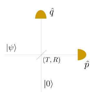
Figure 6: Schematic representation of eight-port homodyne measurement. The $\hat{p}$ and $\hat{q}$ measurement are each performed by standard homodyne detection.

In this appendix we present the modelization of the eight-port homodyne detection. The input state is mixed with vacuum at a beam splitter characterized by reflectivity $R$ and transmittivity $T$, with $R^{2}+T^{2}=1$. We are interested in showing that this procedure results in projecting the state onto finitely squeezed states. More precisely, we compute the POVM elements

$$\Pi=\frac{1}{c}\ket{\psi(q_{1},p_{2})}\bra{\psi(q_{1},p_{2})}$$ (42)

with

$$\ket{\psi(q_{1},p_{2})}=\frac{1}{N}\bra{0}U_{\text{BS}}\ket{q_{1},p_{2}},$$ (43)

where $\ket{q_{1}}$ and $\ket{p_{2}}$ are the position and momentum eigenstates

$$\hat{q}_{1}\ket{q_{1}}=\hat{q}_{1}\ket{q_{1}}$$ (44)

$$\hat{p}_{2}\ket{p_{2}}=\hat{p}_{2}\ket{p_{2}}$$ (45)

and the symplectic action of a beam splitter is given by

$$U_{\text{BS}}\begin{pmatrix}\hat{q}_{1}\\ \hat{q}_{2}\end{pmatrix}U_{\text{BS}}^{\dagger}=\begin{pmatrix}T&-R\\ R&T\end{pmatrix}\begin{pmatrix}\hat{q}_{1}\\ \hat{q}_{2}\end{pmatrix}$$ (46)

$$U_{\text{BS}}\begin{pmatrix}\hat{p}_{1}\\ \hat{p}_{2}\end{pmatrix}U_{\text{BS}}^{\dagger}=\begin{pmatrix}T&-R\\ R&T\end{pmatrix}\begin{pmatrix}\hat{p}_{1}\\ \hat{p}_{2}\end{pmatrix}.$$ (47)

$N$ is a normalization constant. Eq.(43) can be directly computed by Fourier transforming the ket $\ket{p_{2}}=\int dq_{2}e^{iq_{2}p_{2}}\ket{q_{2}}$, yielding

$$\ket{\psi(q_{1},p_{2})} =\frac{1}{N}e^{iq_{2}p_{2}}\int\mathrm{d}q_{2}\bra{0}U_{\text{BS}}\ket{q_{1},q_{2}}$$ (48)

$$=\frac{1}{N}\int\mathrm{d}q_{2}e^{iq_{2}p_{2}}\bra{0}Tq_{1}+Rq_{2},-Rq_{1}+Tq_{2}\rangle$$

$$=\frac{1}{N}\int\mathrm{d}q_{2}e^{-\frac{(-Rq_{1}+Tq_{2})^{2}}{2}+iq_{2}p_{2}}\ket{Tq_{1}+Rq_{2}},$$

where we have used that the wave function of the vacuum state in the position representation is

$$\bra{q}0\rangle=\frac{e^{-\frac{s^{2}}{2}}}{\pi^{1/4}},$$ (49)

and we have absorbed the factor $\pi^{1/4}$ in the normalization constant. We use now the change of variables

$$\frac{T}{R}q=-Rq_{1}+Tq_{2},$$ (50)

from which, using $Tq_{1}+\frac{R^{2}}{T}q_{1}+q=q+\frac{q_{1}}{T}$, we obtain

$$\ket{\psi(q_{1},p_{2})} =\frac{e^{i\frac{R}{T}q_{1}p_{2}}}{N}\int\mathrm{d}qe^{-\frac{1}{2}\left(\frac{T}{R}\right)^{2}\hat{q}^{2}}e^{+i\frac{p_{2}}{R}\hat{q}}\ket{q+\frac{q_{1}}{T}}$$

$$\propto e^{i\frac{p_{2}}{R}\hat{q}}e^{-i\frac{q_{1}}{T}\hat{p}}\int\mathrm{d}qe^{-\frac{1}{2}\left(\frac{T}{R}\right)^{2}\hat{q}^{2}}\ket{q}$$ (51)

where we have used $\ket{q+\frac{q_{1}}{T}}=e^{-i\frac{q_{1}}{T}\hat{p}}\ket{q}$. In Eq.(A) we recognize (apart from an irrelevant global phase factor) a squeezed state $\hat{S}(\frac{R}{T})\ket{0}\propto\int dqe^{-\frac{1}{2}\left(\frac{T}{R}\right)^{2}\hat{q}^{2}}\ket{q}$, to which the displacement $\hat{D}\left(\frac{1}{\sqrt{2}}\left(\frac{q_{1}}{T}+i\frac{p_{2}}{R}\right)\right)\propto e^{i\frac{p_{2}}{R}\hat{q}}e^{-i\frac{q_{1}}{T}\hat{p}}$ is applied. This shows that indeed eight-port homodyne detection results in projection onto displaced squeezed states $\hat{D}(x)\hat{S}(r)\ket{0}$ with $x=\frac{1}{\sqrt{2}}\left(\frac{q_{1}}{T}+i\frac{p_{2}}{R}\right)$ and $r=R/T$.

References

- Aaronson and Arkhipov (2013) S. Aaronson and A. Arkhipov, Theory of Computing 9, 143 (2013).
- Bremner et al. (2010) M. J. Bremner, R. Josza, and D. Shepherd, Proc. R. Soc. A 459, 459 (2010).
- Bremner et al. (2016) M. J. Bremner, A. Montanaro, and D. J. Shepherd, Phys. Rev. Lett. 117, 080501 (2016).
- Farhi and Harrow (2016) E. Farhi and A. W. Harrow, arXiv:1602.07674 (2016).
- Morimae et al. (2014) T. Morimae, K. Fujii, and J. F. Fitzsimons, Phys. Rev. Lett. 112, 130502 (2014).
- Yokoyama et al. (2013) S. Yokoyama, R. Ukai, S. C. Armstrong, C. Sornphiphatphong, T. Kaji, S. Suzuki, J.-i. Yoshikawa, H. Yonezawa, N. C. Menicucci, and A. Furusawa, Nature Photonics 7, 982 (2013).
- Yoshikawa et al. (2016) J.-i. Yoshikawa, S. Yokoyama, T. Kaji, C. Sorphiphatphong, Y. Shiozawa, K. Makino, and A. Furusawa, arXiv:1606.06688 (2016).
- Bartlett et al. (2002) S. D. Bartlett, B. C. Sanders, S. L. Braunstein, and K. Nemoto, Phys. Rev. Lett. 88, 097904 (2002).
- Mari and Eisert (2012) A. Mari and J. Eisert, Phys. Rev. Lett. 109, 230503 (2012).
- Soto and Claverie (1983) F. Soto and P. Claverie, Journal of Mathematical Physics 24, 97 (1983).
- Rahimi-Keshari et al. (2016) S. Rahimi-Keshari, T. C. Ralph, and C. M. Caves, Phys. Rev. X 6, 021039 (2016).
- Lund et al. (2014) A. P. Lund, A. Laing, S. Rahimi-Keshari, T. Rudolph, J. L. O’Brien, and T. C. Ralph, Phys. Rev. Lett. 113, 100502 (2014).
- Hamilton et al. (2016) C. S. Hamilton, R. Kruse, L. Sansoni, S. Barkhofen, C. Silberhorn, and I. Jex, arXiv:1612.01199v1 (2016).
- Douce et al. (2017) T. Douce, D. Markham, E. Kashefi, E. Diamanti, T. Coudreau, P. Milman, P. van Loock, and G. Ferrini, Phys. Rev. Lett. 118, 070503 (2017).
- Douce et al (2017) T. Douce et al, in preparation (2017).
- Chakhmakhchyan and Cerf (2017) L. Chakhmakhchyan and N. Cerf, arXiv:1705.05299 (2017).
- Lund et al. (2017) A. P. Lund, S. Rahimi-Keshari, and T. C. Ralph, Phys. Rev. A 96, 022301 (2017).
- Leonhardt (2010) U. Leonhardt, Essential Quantum Optics (Cambridge University Press, Cambridge, UK, 2010), 1st ed.
- Olson et al. (2015) J. P. Olson, K. P. Seshadreesan, K. R. Motes, P. P. Rohde, and J. P. Dowling, Phys. Rev. A 91, 022317 (2015).
- Ra et al. (2017) Y.-S. Ra, C. Jacquard, A. Dufour, C. Fabre, and C. Treps, arXiv:1702.02082 (2017).
- Beck (2000) M. Beck, Phys. Rev. Lett. 84, 5748 (2000).
- Ferrini et al. (2013) G. Ferrini, J. P. Gazeau, T. Coudreau, C. Fabre, and N. Treps, New J. Phys. 15, 093015 (2013).
- Paris et al. (2003) M. G. A. Paris, M. Cola, and R. Bonifacio, Phys. Rev. A 67, 042104 (2003).
- Dutta et al. (1995) B. Dutta, N. Mukunda, R. Simon, et al., Pramana 45, 471 (1995).
- Caianiello (1953) E. R. Caianiello, Il Nuovo Cimento (1943-1954) 10, 1634 (1953).
- Stockmeyer (1985) L. Stockmeyer, SIAM Journal on Computing 14, 849 (1985).
- Lautemann (1983) C. Lautemann, Information Processing Letters 17, 215 (1983).
- Toda (1991) S. Toda, SIAM Journal on Computing 20 (1991).
- Roslund et al. (2014) J. Roslund, R. Medeiros de Araújo, S. Jiang, C. Fabre, and N. Treps, Nature Photonics 8, 109 (2014).
- de Araújo et al. (2014) R. M. de Araújo, J. Roslund, Y. Cai, G. Ferrini, C. Fabre, and N. Treps, Phys. Rev. A 89, 053828 (2014).
- Helgason (1978) S. Helgason, Differential geometry, Lie groups, and Symmetric spaces (Academic Press, 1978).
- Arzani et al (2017) F. Arzani et al, in preparation (2017).
- Neville et al. (2017) A. Neville, C. Sparrow, R. Clifford, E. Johnston, P. M. Birchall, A. Montanaro, and A. Laing, arXiv:1705.00686 (2017).
- Clifford and Clifford (2017) P. Clifford and C. Clifford, arXiv:1706.01260 (2017).
- Seshadreesan et al. (2015) K. P. Seshadreesan, J. P. Olson, K. R. Motes, P. P. Rohde, and J. P. Dowling, Phys. Rev. A 91, 022334 (2015).
- Rohde et al. (2015) P. P. Rohde, K. R. Motes, P. Knott, J. Fitzsimons, J. Munro, and J. P. Dowling, Phys. Rev. A 91, 012342 (2015).