Strongly correlated one-dimensional Bose-Fermi quantum mixtures: symmetry and correlations

Abstract

We consider multi-component quantum mixtures (bosonic, fermionic, or mixed) with strongly repulsive contact interactions in a one-dimensional harmonic trap. In the limit of infinitely strong repulsion and zero temperature, using the class-sum method, we study the symmetries of the spatial wave function of the mixture. We find that the ground state of the system has the most symmetric spatial wave function allowed by the type of mixture. This provides an example of the generalized Lieb-Mattis theorem. Furthermore, we show that the symmetry properties of the mixture are embedded in the large-momentum tails of the momentum distribution, which we evaluate both at infinite repulsion by an exact solution and at finite interactions using a numerical DMRG approach. This implies that an experimental measurement of the Tan’s contact would allow to unambiguously determine the symmetry of any kind of multi-component mixture.

1 Introduction

Ultracold atom experiments allow to engineer and probe, with an incredible and always-improving precision, a yet inaccessible variety of many-body quantum systems [1]. One-dimensional (1D) models, which display several unique features associated to the reduced dimensionality [2], are the object of intense theoretical and experimental interest. Quantum gases in one dimension can be realized in actual experiments by trapping atoms in tight optical waveguides [3, 4, 5, 6]. Moreover, these experiments offer the possibility to tune the interactions between the atoms [1, 7], and hence to access the strongly correlated regime for various kinds of quantum mixtures. For instance, a strongly repulsive two-component 1D Fermi gas was realized in [8], and a mixture with up to six fermionic components was realized using Ytterbium atoms [6]. Other experiments with Ytterbium isotopes offer promising perspectives for the realization of strongly interacting 1D Bose-Fermi mixtures [9].

In multi-component Bose-Fermi quantum mixtures, the exchange symmetry between identical particles is fixed by their bosonic or fermionic nature, but not between distinguishable particles. Thus, a natural question is to find how to characterize, both theoretically and experimentally, the global exchange symmetry of the many-body wave-function. This fundamental property is directly related to the magnetic properties of the system [10, 11, 12]. Therefore, strongly interacting 1D atomic mixtures appear to be a perfect experimental and theoretical playground for studying quantum magnetism [13]. They also offer the opportunity to study itinerant magnetism phases, i.e. magnetism without a lattice [14].

A typical feature in strongly interacting gases is the so-called fermionization: at increasing repulsive interactions, particles which are not subjected to the Pauli principle tend to avoid each other. In the limit of infinite repulsion, contact interactions mimic the Pauli exclusion principle, e.g. they induce zeros in the many-body wave function when two particles meet. This phenomenon allows the construction of an exact solution for any type of quantum mixture through a mapping onto a non-interacting spinless Fermi gas [15, 16, 17, 18, 11, 19].

In this work, we focus on 1D multi-component Bose-Fermi quantum mixtures with strongly repulsive contact interactions, taking the experimentally relevant case of a harmonic external confinement. In the limit of infinite interactions, we provide an exact solution of the multi-component mixture with arbitrary number of components using the method developed in [11, 19]. In order to address the symmetry of the many-body wave function of the ground and excited states we use the class-sum method. We show that the mixtures obey a generalized version of the Lieb-Mattis theorem [20]. Namely, as obtained for multi-component fermions in [21], the spatial ground state wave function of each system is the most symmetric one. Our analysis of the symmetries also confirms the ordering of the excited states recently obtained in [22] for fermionic mixtures and extends this concept to the case of Bose-Fermi mixtures. Furthermore, we explore how symmetry affects the properties of the system in coordinate and momentum space by studying density profiles and momentum distributions. For this purpose we combine the exact solution at infinite interactions with numerical Density Matrix Renormalization Group (DMRG) calculations at finite interactions. This allow us to analyze the symmetry structure of the mixture in the fermionization process. In particular, we show that a precise measurement of the asymptotic momentum distribution would allow to probe the symmetry of the mixture, thus generalizing our previous result on multi-component fermions [23].

The paper is organized as follows: In Section 2, we give a description of our model and of its solution. Then, in Section 3, we provide a detailed description of the class-sum method that we use to extract the exchange symmetry of the many-body wave function. In Section 4, we provide our results for the density profiles and momentum distributions. Finally, Sec. 5 gives our concluding remarks and perspectives.

2 Model and general solution

We consider a mixture of $N_{B}=N_{1}^{B}+\ldots+N_{b}^{B}$ bosons and $N_{F}=N_{1}^{F}+\ldots+N_{f}^{F}$ fermions, with $N=N_{B}+N_{F}$, divided in $b$ and $f$ flavors (e.g. spin components), all having the same mass $m$. For a Bose-Fermi mixture this is always an approximation, which is appropriate e.g. for mixtures of isotopes. This type of mixtures is experimentally accessible with Ytterbium atoms [9] for instance. The particles are confined in a tight atomic waveguide so that their motion can be considered one-dimensional. Their positions are given by the coordinates $x_{1}^{B,1},\ldots,x_{N_{B}}^{B,b},x_{N_{B}+1}^{F,1},\dots,x_{N}^{F,f}$. For the sake of simplicity of notations, the exponents specifying the type and flavor of the particle will be from now on omitted. All the particles are also subjected to the same one-dimensional confinement $V(x)=\frac{1}{2}m\omega^{2}x^{2}$, which could be realized e.g. in cigar-shaped optical traps. The interactions between the particles are modelled via the pseudo-potential $V_{\mathrm{int}}(x,y)=g\delta(x-y)$. Here $g=-2\hbar^{2}/ma_{1D}$, and $a_{1D}$ is the 1D effective scattering length [7], which accurately describes the $s$-wave scattering dominated collisions in a restricted geometry at low enough energies and densities [1]. We assume that the boson-boson, boson-fermion and fermion-fermion interactions are characterized by the same interaction strength $g$. In the fermionic case, no $s$-wave collisions occur among fermions belonging to the same flavor. The Hamiltonian describing the system is then given by

$$H=\sum_{i=1}^{N}\left(-\frac{\hbar^{2}}{2m}\frac{\partial^{2}}{\partial x_{i}^{2}}+\frac{1}{2}m\omega^{2}x_{i}^{2}\right)\ +g\sum_{1\leq i<j\leq N}\delta(x_{i}-x_{j}).$$ (1)

The interaction term in $H$ is equivalent to imposing the cusp condition on the many-body wave function $\Psi=\Psi(x_{1},\ldots,x_{N})$,

$$\partial_{x}\Psi(x=0^{+})-\partial_{x}\Psi(x=0^{-})=\frac{mg}{\hbar^{2}}\,\Psi(x=0)\ ,$$ (2)

where $x=x_{i}-x_{j}$.

2.1 Exact many-body wave function at infinite repulsion

As a consequence of the cusp condition, in the strongly correlated limit $g\to\infty$, the many-body wave function vanishes whenever $x_{i}=x_{j}$, leading to fermionization features. In this limit one can build an exact many-body wave function satisfying the cusp condition by taking [11, 16]

$$\Psi(x_{1},\ldots,x_{N})=\sum_{P\in S_{N}}a_{P}\theta_{P}(x_{1},\ldots,x_{N})\Psi_{A}(x_{1},\ldots,x_{N}),$$ (3)

where $S_{N}$ is the permutation group of $N$ elements, $\theta_{P}(x_{1},\ldots,x_{N})$ is equal to $1$ if $x_{P(1)}<\cdots<x_{P(N)}$ (coordinate sector, later indicated as $(P(1),P(2),...P(N))$) and $0$ otherwise, and $\Psi_{A}$ is the fully antisymmetric fermionic wave function $\Psi_{A}(x_{1},\ldots,x_{n})=\frac{1}{\sqrt{N!}}\mathrm{det}[\phi_{i-1}(x_{j})]_{i,j=1,\ldots,N}$ where $\phi_{0},\ldots,\phi_{N-1}$ are the eigenfunctions of the single particle Hamiltonian $H_{1}=-(\hbar^{2}/2m)\partial_{x}^{2}+V(x)$. The coefficients $a_{P}$ in Eq.(3) corresponding to exchange of particles belonging to the same bosonic (fermionic) component of the mixture are such that $a_{P}=1$ ($a_{P}=-1$) respectively. Hence, the number of independent coefficients is reduced to $D_{N,\mathrm{b+f}}=\frac{N!}{N_{1}!\ldots N_{\mathrm{b+f}}!}$. This allows to extremely reduce the cost of calculations, by identifying sectors that are equal modulo permutations of identical particles. This smaller basis is often called the snippet basis [16, 18]. In this paper, we will switch from one formalism to the other depending on whether a distinction between identical bosons is necessary or not.

In order to find the coefficients $a_{P}$ we use the variational approach developed in [11]. This is based on a strong-coupling expansion of the energy to order $1/g$, i.e. by setting $E=E_{A}-K/g$ where $E_{A}$ is the fermionic energy associated with $\Psi_{A}$. Using the Hellmann-Feynman theorem together with (2) we obtain

$$K=g\left<H_{\mathrm{int}}\right>=\sum_{P,Q\in S_{N}}(a_{P}-a_{Q})^{2}\alpha_{P,Q},$$ (4)

where $\alpha_{P,Q}=\int\mathrm{d}x_{1}\ldots\mathrm{d}x_{N}\theta_{\mathrm{Id}}(x_{1},\ldots,x_{N})\delta(x_{k}~{}-~{}x_{k+1})\left[\partial\Psi_{A}/\partial x_{k}\right]^{2}\equiv\alpha_{k}$ if $P$ and $Q$ are equal up to a transposition $\tau_{k}$ of two consecutive particles that are either distinguishable particles or indistinguishable bosons at positions $k$ and $k+1$, and $0$ otherwise (see [21, 10] for computational methods). Note that the spatial parity of the trap implies that $\alpha_{k}=\alpha_{N-k}$ for all $k$. Then, the variational condition $\partial K/\partial a_{P}=0$ is shown to be equivalent to a simple diagonalization problem $V\mathbf{a}_{\mathrm{snip}}=K\mathbf{a}_{\mathrm{snip}}$, where $\mathbf{a}_{\mathrm{snip}}$ is the vector of the $D_{N,\mathrm{b+f}}$ independent $a_{i}$ coefficients and $V$ is a $D_{N,\mathrm{b+f}}\times D_{N,\mathrm{b+f}}$ matrix defined in the snippet basis by

$$V_{ij}=\left\{\begin{array}[]{ll}-\alpha_{i,j}&\mbox{if }i\neq j\\ \sum_{\mathrm{d},k\neq i}\alpha_{i,k}+2\sum_{\mathrm{b},k\neq i}\alpha_{i,k}&\mbox{if }i=j\end{array}\right.,$$ (5)

where the index $\mathrm{d}$ means that the sum has to be taken over snippets $k$ that transpose distinguishable particles as compared to snippet $i$, while $\mathrm{b}$ means that the sum is taken over sectors that transpose identical bosons. The highest eigenvalue of $V$ yields the ground state of the system, whereas the other eigenvalues correspond to all the excited states that belong to the same $D_{N,\mathrm{b+f}}$-degenerate manifold at $g\rightarrow\infty$.

3 Symmetry of the mixture

In this section, we study the spatial symmetry of our solution under exchange of particles. To this purpose we use the class-sum method, inspired from nuclear physics [24, 25], and previously used in [18, 21, 23].

3.1 General method

We consider a $N$-particle wave function $\Psi(x_{1},\dots,x_{N})$, identified by a vector $\mathbf{a}_{\mathrm{sect}}=(a_{1},\dots,a_{N!})$ as in Eq. (3). We want to determine its permutational symmetry, i.e. find to which irreducible representation(s) of the permutation group $S_{N}$ it belongs. Each irreducible representation can be labeled by a Young diagram, where, according to the standard notation, boxes in the same column (resp. row) correspond to an antisymmetric (resp. symmetric) exchange of particles [26]. Examples of Young diagrams and their corresponding symmetries for $N=4$ are given in Table 1. Using the Young diagrams, it is possible to know a priori, given a configuration $N_{1}^{B}+\ldots+N_{b}^{B}+N_{1}^{F}+\ldots+N_{f}^{F}$, which irreducible representations are possible for $\Psi$, compatible with the antisymmetrization of fermions belonging to the same component, and symmetrization for same-component bosons. More precisely, in order to build the standard Young tableaux for a given mixture, we index by a letter the particles of each given species. We therefore order the species by decreasing order and label them alphabetically. We then label the boxes of the Young diagrams imposing that the entries of each row and column are always increasing (in weak sense), and with the symmetry constraint that no more than one same-component bosonic/fermionic label can be present in one column/row. Examples are provided for $4$-particle mixtures in Table 1.

Exchange symmetry	Young diagram(s)
symmetric
antisymmetric
mixed

Mixture	Young tableaux
$2^{B}(a)+2^{B}(b)$	$a$ $a$ $b$ $b$     $a$ $a$ $b$     $b$     $a$ $a$     $b$ $b$
$2^{F}(a)+2^{F}(b)$	$a$     $a$     $b$     $b$     $a$ $b$     $a$     $b$     $a$ $b$     $a$ $b$
$2^{B}(a)+2^{F}(b)$	$a$ $a$ $b$     $b$     $a$ $a$     $b$     $b$

Table 1: Young diagrams and standard Young tableaux for different two-component mixtures with $N=4$. The particles of the species are labeled $a$ resp. $b$, and can be either bosonic or fermionic.

We also recall that the number of standard Young tableaux corresponding to a given Young diagram is equal to the dimension of the associated irreducible representation [27]. The number $d_{\lambda}$ of possible standard Young tableaux associated with a Young diagram $\lambda$ is given by the Hook-length formula

$$d_{\lambda}=\prod_{(i,j)\in\mu}\frac{N!}{h_{\lambda}(i,j)},$$ (6)

where $h_{\lambda}(i,j)$ is equal to the number of cells below the box $(i,j)$ + the number of cells at the right of the box $(i,j)$ + 1. Interestingly, the dimension $d_{\lambda}$ counts the number of energy eigenstates having the symmetry $\lambda$ [28, 29].

In order to obtain the symmetry associated with a given wave function $\Psi(x_{1},\dots,x_{N})$ belonging to the degenerate manifold, we define a set of $N!\times N!$ matrices whose eigenvalues are directly connected to the irreducible representations of $S_{N}$, namely the conjugacy class-sums [27, 30]. Considering cycles $\sigma$ of length $|\sigma|=p$, which permute $p$ elements of $\{1,\dots,N\}$ in a cyclic way, the $p$-cycle class-sum $\Gamma^{(p)}$ is represented in the coordinate-sector basis of $N$ non-interacting fermions as

$$\Gamma^{(p)}=\sum_{\sigma,|\sigma|=p}M_{\sigma}.$$ (7)

$M_{\sigma}$ is an $N!\times N!$ matrix whose elements are $\left(M_{\sigma}\right)_{PQ}=(-1)^{|\sigma|-1}\delta_{P,\sigma\circ Q}$, and the factor $(-1)^{|\sigma|-1}$ is due to the inherent antisymmetry of the basis. As an example, for $N=3$, taking as basis $\left((1,2,3),(1,3,2),(2,1,3),(2,3,1),(3,1,2),(3,2,1)\right)$, one has

$$\Gamma^{(2)}=\begin{pmatrix}0&-1&-1&0&0&-1\\ -1&0&0&-1&-1&0\\ -1&0&0&-1&-1&0\\ 0&-1&-1&0&0&-1\\ 0&-1&-1&0&0&-1\\ -1&0&0&-1&-1&0\\ \end{pmatrix},$$ (8)

and

$$\Gamma^{(3)}=\begin{pmatrix}0&0&0&1&1&0\\ 0&0&1&0&0&1\\ 0&1&0&0&0&1\\ 1&0&0&0&1&0\\ 1&0&0&1&0&0\\ 0&1&1&0&0&0\\ \end{pmatrix}.$$ (9)

The key point of our method is that the class-sum eigenvalues $\gamma^{(p)}$ are directly related to the irreducible representations of $S_{N}$: given a Young diagram $\lambda=[\lambda_{1},\ldots,\lambda_{n}]$, where $\lambda_{i}$ is the number of boxes in row $i$, the following relation holds [31]:

$$\gamma^{(p)}=\frac{1}{p}\sum_{i=1}^{n}\mu_{i}(\mu_{i}-1)\ldots(\mu_{i}-p+1)\prod_{j\neq i}\frac{\mu_{i}-\mu_{j}-p}{\mu_{i}-\mu_{j}}.$$ (10)

where $\mu_{i}=\lambda_{i}-i+n$. The fundamental reason behind the above connection (10) between class sums and Young tableaux is that there is a one-to-one correspondence of the eigenvalues of a class-sum and the characters of the irreducible representations of $S_{N}$ [25, 30]. Once one considers the relation between the irreducible representations of $S_{N}$ and the ones of $SU(\kappa)$ (for the case of $\kappa$-species mixtures) [26], it is possible to connect the eigenvalues of the class-sum operators and those of the $SU(\kappa)$ Casimir operators. The latter are the ones that, roughly speaking, describe the character of $SU(\kappa)$ irreps. and thus generalise the $SU(2)$ concept of spin length.

Using the above properties, in order to determine the symmetry of the wave function $\Psi$ of a given mixture we proceed as follows: first, we determine the matrix $\Gamma^{(2)}$ on the coordinate-sector basis and compute its eigenvalues $\gamma^{(2)}$. Then, we list all the Young diagrams allowed within the given type of mixture, and using Eq. (10), we associate each eigenvalue $\gamma^{(2)}$ to a given Young diagram. If different diagrams correspond to the same $\gamma^{(2)}$, we repeat this operation to higher order in the size $p$ of the cycles until there are no longer degeneracies. Finally, we expand the wave function $\Psi$, represented in the same basis as the vector $\mathbf{a}_{\mathrm{sect}}=(a_{1},\dots,a_{N!})$, on the basis of the eigenvectors of $\Gamma^{(p)}$ in order to determine the weights of the different irreducible representations, and hence the symmetry content of the wave function.

Finally, we would like to comment that the class-sum method has been here adapted to the ansatz (3), but it can be used as well for other ansatz, e.g. the Bethe ansatz [32, 12], as long as the $M_{\sigma}$ matrices in Eq. (7) are defined correspondingly.

3.2 Results and discussion

The case of fermionic mixtures has already been studied in [21, 23], and the case of simple Bose-Fermi mixtures $N_{1}^{B}+N_{1}^{F}$ with $N_{1}^{B}=N_{1}^{F}$ was studied in [18]. In this work, we extend these results to the more complex and general case of Bose-Fermi mixtures with more than one bosonic/fermionic components. In particular, we study the cases $2^{B}+2^{F}$, $3^{B}+3^{F}$, $2^{B}+2^{B}+2^{F}$ and $2^{B}+2^{F}+2^{F}$. Note that we only need $p_{\mathrm{max}}=3$ in order to discriminate between                            and                       or between                                 and                            , which are degenerate in $\Gamma^{(2)}$. We focus on the ground states of a given symmetry configuration, in the sense that, given a symmetry $S$, they have the highest eigenvalue of $V$ denoted $K(S)$, corresponding to the the lowest energy $E(S)$. Our results are shown in Table 2.

Mixture	Symmetry	$\gamma^{(2)}$	$K(S)/(\hbar^{2}\omega^{2}a_{ho})$
$2^{B}+2^{F}$		2	10.66
		-2	7.08
$3^{B}+3^{F}$		3	30.37
		-3	24.43

(a) Two-component mixtures.

Mixtures	Symmetry	$\left(\gamma^{(2)},\gamma^{(3)}\right)$	$K(S)/(\hbar^{2}\omega^{2}a_{ho})$
$2^{B}+2^{B}+2^{F}$		$\left(9,16\right)$	33.35
$2^{B}+2^{F}+2^{F}$		$\left(5,0\right)$	32.16
		$\left(3,-8\right)$	30.63
		$\left(3,4\right)$	30.37
		$\left(0,-5\right)$	28.96
		$\left(-3,-8\right)$	24.97
		$\left(-3,4\right)$	24.43
		$\left(-5,0\right)$	22.69
		$\left(-9,16\right)$	14.60

(b) Three-component mixtures: Young tableaux in black are the possible ones for both mixtures whereas the blue (red) ones are restricted to the $2^{B}+2^{B}+2^{F}$ ($2^{B}+2^{F}+2^{F}$) mixture.

Table 2: (Color online) Symmetries diagrams obtained for different states and different mixtures, with their corresponding class-sum eigenvalues $\left(\gamma^{(2)},\gamma^{(3)},\ldots,\gamma^{(p_{\mathrm{max}})}\right)$ and their energy slopes $K(S)$ in units of $\hbar^{2}\omega^{2}a_{ho}$.

First, we observe that, as in the case of Fermi mixtures [21], these states have a pure symmetry, i.e. they belong to a unique irreducible representation. Moreover, a direct comparison of Table 2(a) and Table 2(b) shows that Bose-Fermi mixtures with more than two components have much complex symmetric structures than the two-component ones, the latter having always only two possible symmetries [18]. Another interesting observation is that a given symmetry $S$ corresponds to the same ground state energy slope $K(S)$, independently of the mixture. In that sense, the symmetry of the mixture appears to be a deeper physical characterization than the actual choice of the mixture.

Furthermore, it is clear in Table 2 that diagrams with higher $K(S)$ or, equivalently, lower $E(S)$, are more “horizontal”, or more “symmetric”. In the context of a two-spin component fermionic mixture, this observation is known as the Lieb-Mattis theorem and has very strong implications in the theory of ferromagnetism [20]. It states that the mixture with the lowest total spin, and therefore the most symmetric spatial wave-function, will display the lowest ground-state energy, which implies that the ground state is unmagnetized. On the other hand, it was proven in [33] that the ground state of an interacting bosonic mixture is always fully polarized, which again is equivalent to the property that the spatial wave function is the most symmetric. Our results show that the ground state corresponds to the most symmetric spatial configuration allowed by the Bose-Fermi mixture, generalizing the results obtained in the case of purely fermionic mixtures in [21, 23], in agreement with the second Lieb-Mattis Theorem (LMT II) [20].

The notion that a state $S$ is “more symmetric” than $S^{\prime}$ is usually understood in the sense of the so-called pouring principle, which in terms of Young diagrams means that the diagram corresponding to $S$ can be poured into the diagram corresponding to $S^{\prime}$ by moving boxes up and right [20]: e.g.                       can be poured into                       . The LMT II claims that $E(S)>E(S^{\prime})$ if $S$ can be poured in $S^{\prime}$. Nevertheless the pouring principle has its limitations: clearly                            and                       can not be compared according to this principle. Here, we show that these symmetries display different interaction energies and are therefore comparable (e.g. $K\left({\tiny\hbox{}\vbox{\vbox{\offinterlineskip\vbox{\hrule height=0.3pt\hbox{\vrule height=4.37334pt,width=0.3pt,depth=1.0933pt\hbox to5.46666pt{\hfil}\vrule height=4.37334pt,width=0.3pt,depth=1.0933pt\hbox to5.46666pt{\hfil}\vrule height=4.37334pt,width=0.3pt,depth=1.0933pt\hbox to5.46666pt{\hfil}\vrule height=4.37334pt,width=0.3pt,depth=1.0933pt\hbox to5.46666pt{\hfil}\vrule height=4.37334pt,width=0.3pt,depth=1.0933pt} \hrule height=0.3pt}\vspace{-\y@linethick} \vbox{\hrule height=0.3pt\hbox{\vrule height=4.37334pt,width=0.3pt,depth=1.0933pt\hbox to5.46666pt{\hfil}\vrule height=4.37334pt,width=0.3pt,depth=1.0933pt} \hrule height=0.3pt}\vspace{-\y@linethick} \vbox{\hrule height=0.3pt\hbox{\vrule height=4.37334pt,width=0.3pt,depth=1.0933pt\hbox to5.46666pt{\hfil}\vrule height=4.37334pt,width=0.3pt,depth=1.0933pt} \hrule height=0.3pt}\vspace{-\y@linethick} }}}\right)<K\left({\tiny\hbox{}\vbox{\vbox{\offinterlineskip\vbox{\hrule height=0.3pt\hbox{\vrule height=4.37334pt,width=0.3pt,depth=1.0933pt\hbox to5.46666pt{\hfil}\vrule height=4.37334pt,width=0.3pt,depth=1.0933pt\hbox to5.46666pt{\hfil}\vrule height=4.37334pt,width=0.3pt,depth=1.0933pt\hbox to5.46666pt{\hfil}\vrule height=4.37334pt,width=0.3pt,depth=1.0933pt} \hrule height=0.3pt}\vspace{-\y@linethick} \vbox{\hrule height=0.3pt\hbox{\vrule height=4.37334pt,width=0.3pt,depth=1.0933pt\hbox to5.46666pt{\hfil}\vrule height=4.37334pt,width=0.3pt,depth=1.0933pt\hbox to5.46666pt{\hfil}\vrule height=4.37334pt,width=0.3pt,depth=1.0933pt\hbox to5.46666pt{\hfil}\vrule height=4.37334pt,width=0.3pt,depth=1.0933pt} \hrule height=0.3pt}\vspace{-\y@linethick} }}}\right)$), confirming the ordering observed in [22] in the case of a Fermi gas and extending the analysis to the case of Bose-Fermi mixtures.

4 Density profiles and momentum distributions

This section is dedicated to the study of the effect of symmetries on the one-body density matrix $\rho_{\nu}(x,y)$ in the strongly interacting regime. For any component $\nu\in{1,\ldots,\mathrm{b+f}}$, $\rho_{\nu}(x,y)$ is defined by

$$\rho_{\nu}(x,y)=N_{\nu}\int\mathrm{d}x_{2}\ldots\mathrm{d}x_{N}\Psi^{*}(x,x_{2},\ldots,x_{N})\Psi(y,x_{2},\ldots,x_{N}),$$ (11)

where the first coordinate of $\Psi$ is chosen to belong to species $\nu$. The one-body density matrix measures the first-order spatial coherence among two particles of species $\nu$ in positions $x$ and $y$ respectively. From the knowledge of the one-body density matrix one can obtain the density profile, according to

$$n_{\nu}(x)=\rho_{\nu}(x,x).$$ (12)

This quantity measures the probability of finding a particle of species $\nu$ in position $x$. It is accessible in cold-atom experiments via in situ imaging [1].

The momentum distribution $n_{\nu}(k)$ of species $\nu$ is also directly extracted from the one-density matrix by Fourier transform, according to

$$n_{\nu}(k)=\frac{1}{2\pi}\iint\mathrm{d}x\,\mathrm{d}y\,\rho_{\nu}(x,y)e^{-ik(x-y)}.$$ (13)

The momentum distribution is one of the most common observables in cold-atom experiments. All the components of a mixture can be separately measured using spin-resolved time-of-flight techniques [1, 34]. The large-momentum tails of the momentum distribution for each component of a mixture follow a universal $k^{-4}$ law, as first proven for the bosonic Tonks-Girardeau gas in [35, 36]. The weights $\mathcal{C}_{\nu}=\lim_{k\to\infty}k^{4}n_{\nu}(k)$, known as Tan’s contacts, are of primary importance because of their relations to many other physical quantities, as the two-point correlators or the interaction energy, in various quantum mixtures and trapping potential [37, 38, 39, 40, 23]. One of these relations allows to link $\mathcal{C}_{\nu}$ to the interaction energy, and more specifically to the part of the interaction energy to which species $\nu$ contributes. More precisely, if we denote $H_{\mathrm{int},\nu\nu^{\prime}}$ the interaction energy between species $\nu$ and $\nu^{\prime}$, the following relation holds

$$\mathcal{C}_{\nu}=\frac{m^{2}g}{\pi\hbar^{4}}\sum_{\nu^{\prime}}(1+\delta_{\nu\nu^{\prime}})H_{\mathrm{int},\nu\nu^{\prime}}.$$ (14)

4.1 Exact results at infinite interactions

In order to compute the one-body density matrix in the infinitely repulsive case $g\to\infty$, we start from the exact solution for the many-body wave function (3). Few derivation steps allow to reduce the many-body integration in (11) to the calculation of single-particle integrals: we label the $N!$ permutations $P\in S_{N}$ by an index $i_{k}$, where $i\in\{1,\dots,N\}$ denotes the position of the first particle, and $k\in\{1,\dots,(N-1)!\}$ labels the permutations of the $N-1$ other particles. Then, choosing $x\leq y$, Eq. (11) becomes

$$\rho_{\nu}(x,y)=N_{\nu}\sum_{1\leq i\leq j\leq N}R_{\nu}^{(ij)}(x,y),$$ (15)

where

$$R_{\nu}^{(ij)}(x,y)=\int_{S^{(ij)}}\mathrm{d}x_{2}\ldots\mathrm{d}x_{N}\Psi(x,x_{2},\ldots,x_{N})\Psi(y,x_{2},\ldots,x_{N}),$$ (16)

with $S^{(ij)}=\{x_{2}<\dots<x_{i-1}<x<x_{i+1}<\ldots<x_{j-1}<y<x_{j+1}<\ldots<x_{N}\}$. Noticing that $\int\mathrm{d}x_{2}\ldots\mathrm{d}x_{N}\theta_{P_{i_{k}}}(x,\ldots,x_{N})\theta_{P_{i_{l}}}(y,\ldots,x_{N})\propto\delta_{kl}$, we obtain after some algebra [41, 21]:

$$R_{\nu}^{(ij)}(x,y)=C_{ij}\sum_{P,Q\in S_{N-1}}\epsilon(P)\epsilon(Q)\displaystyle{\prod_{l=2}^{N}}\int_{L_{ij}}^{U_{ij}}\mathrm{d}x_{l}(x_{l}-x)(x_{l}-y)\phi_{P(l)-1}(x_{l})\phi_{Q(l)-1}(x_{l}),$$ (17)

where $C_{ij}=\frac{2^{N-1}}{\sqrt{\pi}N!(N-1)!}\cdot\frac{\sum_{k=1}^{(N-1)!}a_{i_{k}}a_{j_{k}}}{(i-1)!(j-i)!(N-j)!}$, and where the integration limits $(L_{ij},U_{ij})$ are given by

$$(L_{ij},U_{ij})=\left\{\begin{array}[]{lll}(-\infty,x)&\mbox{if }l\leq i,\\ (x,y)&\mbox{if }i<l\leq j,\\ (y,+\infty)&\mbox{if }l>j.\end{array}\right.$$ (18)

The density profile is readily obtained as $n_{\nu}(x)=N_{\nu}\sum_{i}R_{\nu}^{(ii)}(x,x)$, and the momentum distribution is obtained by numerically evaluating the Fourier transform (13) for the specific case of Eq.(15).

The exact solution allows also for an independent evaluation of the Tan’s contact using the Tan relation on the interaction energy. Using Eq. (4), we find that the interaction energy $H_{\mathrm{int},\nu\nu^{\prime}}$ is given by

$$H_{\mathrm{int},\nu\nu^{\prime}}=\left\{\begin{array}[]{ll}\frac{\hbar^{4}}{2m^{2}g}\sum_{k=1}^{N-1}\sum_{P\in\sigma_{N}(\nu,\nu^{\prime},k)}(a_{P}-a_{\tau_{k}\circ P})^{2}\alpha_{k}&\mbox{if }\nu\neq\nu^{\prime},\\ \frac{\hbar^{4}}{2m^{2}g}\sum_{k=1}^{N-1}\sum_{1\leq i<j\leq N_{\nu}}\sum_{P\in\sigma_{N}(i,j,k)}(a_{P}-a_{\tau_{k}\circ P})^{2}\alpha_{k}&\mbox{if }\nu=\nu^{\prime},\end{array}\right.$$ (19)

where $\sigma_{N}(\mu,\nu,k)$ is the set of all permutations such that particles in $k$ and $k+1$ positions are from the species $\mu$ and $\nu$ (or are particles $i$ and $j$ for $\sigma_{N}(i,j,k)$), and $\tau_{k}$ is the transposition of these two particles. Note that $H_{\mathrm{int},\nu\nu}=0$ if species $\nu$ is fermionic. The calculation of the interaction energy allows to obtain the Tan’s contact using Eq.(14).

4.2 Numerical solution at arbitrary interactions

In realistic experimental conditions, the interactions are tunable, allowing to explore all the interactions regime from small to large values. In particular, a relevant question is to what extent the density profiles and the momentum distributions evaluated from the exact solution at $g\rightarrow\infty$ describe accurately the ground states at large but finite interaction. In order to tackle the arbitrary interaction regime, we have performed numerical calculations using a two-site optimization scheme, according to the Density-Matrix Renormalization-Group (DMRG) method, based on matrix product states (MPS). The code allows the exploitation of Abelian symmetries (here particle-number conservation for each species). To address the continuous problem, we discretized the relevant region of the trap and calculated properties of the resulting lattice model. The continuum results were then obtained by increasing the number of lattice points in consecutive simulations (thereby decreasing the lattice spacing) and finite-size scaling the quantities of interest. Density distributions were measured as site-occupations in the discretized model; the Tan contacts were determined through the interaction part of the energy. The momentum distributions were obtained from Fourier-transformed two-point correlators $n_{\nu}(k)=\frac{1}{L}\sum_{j,l=1}^{L}e^{i(j-l)k}\langle c_{\nu,j}^{\dagger}c_{\nu,l}\rangle$, where $c_{\nu,j}^{(\dagger)}$ are the annihilation (creation) operators for the species $\nu$ in the lattice model. The maximal number of lattice sites considered was 216, covering a region of 12 harmonical trap lengths. The virtual bond-dimension of the MPS was $m\approx 150$ which appears of be sufficient for the very low density of particles we consider here.

4.3 Density profiles

The density profiles of a multi-component mixture display a wealth of information concerning the intercomponent interactions as well as the magnetic structure.

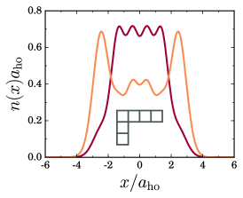
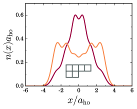
Figure 1: (Color online.) Exact solution for the bosonic (brown) and fermionic (orange) ground state density profiles (in unit of $a_{ho}^{-1}$) in the limit $g\to\infty$, as functions of the spatial coordinate $x/a_{ho}$. From left to right, the mixtures are $3^{B}+3^{F}$, $2^{B}+2^{F}+2^{F}$ and $2^{B}+2^{B}+2^{F}$. For the case of ternary mixtures, the density profiles of the two components with the same statistics and same particle number coincide.

At mean-field level, by increasing the strength of repulsive intercomponent interactions [42] the system is predicted to undergo spatial separation. However, for strong interactions mean-field theory loses its validity due to the change of equation of state and the increased effect of quantum fluctuations. Luttinger liquid theory for a homogeneous system also predicts an instability towards spatial separation [43]. For a binary mixture in a harmonic trap, an analysis based on the local-density approximation of the exact equation of state was performed in [44, 45], yielding a partial spatial separation of the two components at strong interactions. For small particle numbers, and finite interactions, spatial separation was found within some parameter regimes using mapping to a spin model and exact diagonalization in [46], and for finite interactions an exact solution showing spatial separation was obtained in [19].

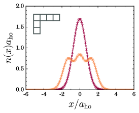
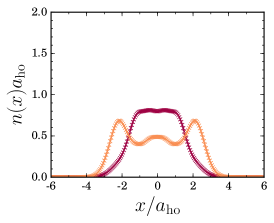
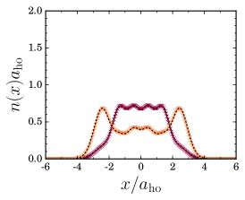
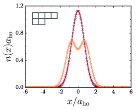
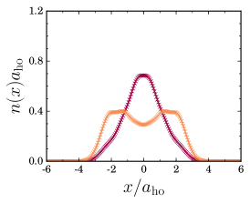
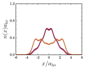
Figure 2: (Color online.) Bosonic (brown) and fermionic (orange) ground state density profiles of a $3^{B}+3^{F}$ mixture (top row) and $2^{B}+2^{F}+2^{F}$ mixture (bottom row) with interactions $g=0.0\,\hbar\omega a_{ho}$ (left), $g=10.0\,\hbar\omega a_{ho}$ (center), and $g=100.0\,\hbar\omega a_{ho}$ (right). In the right panel, the exact solution for $g\rightarrow\infty$ in also shown in dashes.

We present in Figs. 1-2 our results for both binary and ternary multi-component mixtures made of six particles. The results for the binary mixtures agree with [19, 46] in showing spatial separation, with the bosonic component occupying the center of the trap and the fermionic component pushed towards the edges.

The results on spatial separation can be seen as a direct consequence of the generalized Lieb-Mattis theorem. Indeed, if the ground state is the most symmetric configuration allowed by the type of mixture, then it is built in such a way to minimize the number of anti-symmetric exchanges, which is the case if the fermions are on the edges.

For ternary mixtures, at fixed numbers of particles in each component, we find that the details of the density profiles depend on the type of mixture. This shows that the spatial separation is not only an effect of the interactions but also of the symmetry. Also, we remark that the results at finite interactions display the same features as the strongly-correlated regime already at intermediate interactions. This suggests that the spatial symmetry is already present for finite interactions.

4.4 Momentum distributions and Tan’s contact

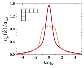
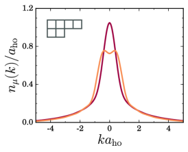
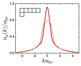
Figure 3: (Color online) Exact solution for bosonic (brown) and fermionic (orange) ground-state momentum distributions (in unit of $a_{ho}$) and as functions of $ka_{ho}$ for $g\to\infty$. From left to right, the mixtures are $3^{B}+3^{F}$, $2^{B}+2^{F}+2^{F}$ and $2^{B}+2^{B}+2^{F}$.

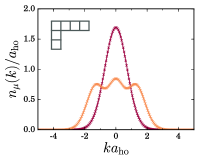
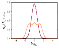
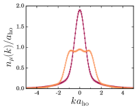
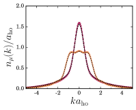
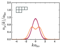
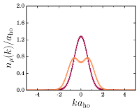
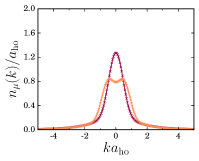
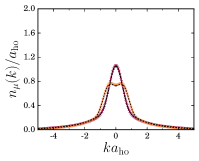
Figure 4: (Color online) Bosonic (brown) and fermionic (orange) ground state momentum profiles of a $3^{B}+3^{F}$ mixture (top row) and a $2^{B}+2^{F}+2^{F}$ mixture (bottom row) with interactions $g=0.0\,\hbar\omega a_{ho}$, $g=1.0\,\hbar\omega a_{ho}$, $g=10.0\,\hbar\omega a_{ho}$ and $g=100.0\,\hbar\omega a_{ho}$ (from left to right). In the right panel, the exact solution for $g\rightarrow\infty$ in also shown in dashes.

We now turn to the discussion of our results for the momentum distribution. Fig. 3 shows our predictions for the regime of infinite interaction strength. The momentum distribution of the bosonic components display one central peak, whereas the fermionic components display as many peaks as the number of the fermions in the corresponding species. This feature, typical of non-interacting spinless fermions in harmonic confinement [47], has also been reported for multi-component interacting fermionic mixtures in harmonic traps [48]. The occurrence of different peaks in the fermionic momentum distribution can be seen as a consequence of the Pauli principle for fermions belonging to the same species.

Fig. 4 shows the dependence of the momentum distributions on interaction strength. At increasing interactions we notice that the number of peaks in each distribution is conserved, and the shape of both fermionic and bosonic momentum distributions looks qualitatively the same. However, a detailed analysis shows that both bosonic and fermionic momentum distributions shrink in their central part. This is complementary to the coordinate space description, where repulsive interactions tend to broaden the profiles. Furthermore, the tails of the momentum distribution become more and more important at increasing interactions, as it is visible on Fig. 4. These tails are shown in Fig. 5 for a finite value of the interaction parameter $g=10.0\,\hbar\omega a_{ho}$ and in Fig. 6 for the limiting case $g\rightarrow\infty$. All the mixtures analysed exhibit the $k^{-4}$ behavior with the expected Tan’s contact coefficients. The asymptotic behaviour of the tails (dashed lines) has been obtained from Eq.(14), where the interaction energy for the mixtures at $g=10.0\,\hbar\omega a_{ho}$ has been numerically calculated (Fig. 5), while for the mixtures at $g\rightarrow\infty$ has been evaluated from the exact solution via Eq. (19) (Fig. 6). For balanced mixtures with the same number of particles in each component we notice that Tan’s contact are not equal for bosonic and fermionic species, at difference from the case of multi-component fermionic mixtures [23]. This properties readily follows from Eq. (19), showing that in the bosonic case there is an additional term corresponding to intracomponent boson-boson interactions.

Finally, we notice that the knowledge of the Tan’s contacts $\mathcal{C}_{\nu}$ for each component of the mixture allows to deduce the symmetry of the mixture, since the total contact $\mathcal{C}_{\mathrm{tot}}=\sum_{\nu=1}^{\mathrm{b+f}}\mathcal{C}_{\nu}$ is linked to the energy slope $K$ via Eq. (4) and (14) through

$$\mathcal{C}_{\mathrm{tot}}=\frac{m^{2}}{\pi\hbar^{4}}K,$$ (20)

and each $K(S)$ corresponds to a unique symmetry $S$ (see Table 2 in Sec. 3). Thus, an experimental measurement of Tan’s contact, e.g. through spin-resolved time-of-flight measurements, or through the energy, would allow a symmetry spectroscopy of the Bose-Fermi mixture [49]. This generalizes our previous results on fermionic mixtures [23].

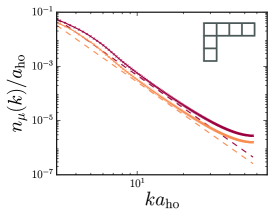
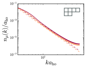
Figure 5: (Color online) Tails of the momentum distributions (brown: bosons, orange: fermions) in a $3^{B}+3^{F}$ mixture (left) and in a $2^{B}+2^{F}+2^{F}$ mixture (right), with interactions $g=10.0\,\hbar\omega a_{ho}$. The dashed lines show the Tan contacts as determined through the interaction energies in Eq. (14). The bending of the momentum curves for very large momenta is an artifact originating from the discretization procedure.

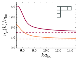
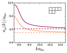
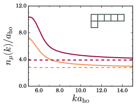
Figure 6: (Color online) Bosonic (brown) and fermionic (orange) ground state $k^{4}n_{\nu}(k)$ functions in unit of $a_{ho}^{-3}$ and as functions of $ka_{ho}$. From left to right, the mixtures are $3^{B}+3^{F}$, $2^{B}+2^{F}+2^{F}$ and $2^{B}+2^{B}+2^{F}$. The horizontal lines are obtained from the exact solution via Eq. (19) in Eq.(14).

5 Conclusions

In this work we have studied the spatial and the momentum distributions of a zero-temperature multi-component boson-fermion mixture, trapped in a one-dimensional harmonic potential. We have considered the ideal case of equal-mass particles and equal contact-interaction strength, that could be obtained in a good approximation in the experiments by trapping and cooling large atomic-number isotopes (e.g. Ytterbium). At infinitely large repulsive interactions we have determined the ground-state properties by using an exact many-body wavefunction. At finite interactions, we have calculated the spatial density profiles and momentum distributions by numerical DMRG methods, obtaining an excellent agreement between the exact calculations and the numerical ones. We have found that at large interactions bosons and fermions are spatially phase separated in the trap and that the momentum distribution tails - the contacts - at fixed number of particles, increase by increasing the number of bosons and/or the number of fermionic components. Both effects are related to the wavefunction symmetry, that we have shown to be, by exploiting a sum-class method, the most possible symmetric one for each type of mixture. Our results are in agreement with a generalized version of the Lieb-Mattis theorem. Importantly, we have found that the exchange symmetry of the many-body wave-function is preserved for large but finite interactions, as in typical experimental conditions, and we have shown that this symmetry is measurable through the tails of the momentum distribution.

References

- Bloch et al. [2008] I. Bloch, J. Dalibard, and W. Zwerger. Many-body physics with ultracold gases. Rev. Mod. Phys., 80:885–964, Jul 2008. doi: 10.1103/RevModPhys.80.885. URL http://link.aps.org/doi/10.1103/RevModPhys.80.885.
- Giamarchi [2003] T. Giamarchi. Quantum Physics in One Dimension. Clarendon Press, Oxford, 2003.
- Moritz et al. [2003] H. Moritz, T. Stöferle, M. Köhl, and T. Esslinger. Exciting collective oscillations in a trapped 1d gas. Phys. Rev. Lett., 91:250402, Dec 2003. doi: 10.1103/PhysRevLett.91.250402. URL https://link.aps.org/doi/10.1103/PhysRevLett.91.250402.
- Paredes et al. [2004] B. Paredes, A. Widera, V. Murg, O. Mandel, S. Fölling, I. Cirac, G. V. Shlyapnikov, T. W. Hänsch, and I. Bloch. Tonks-Girardeau gas of ultracold atoms in an optical lattice. Nature, 429:277, 2004.
- Clément et al. [2009] D. Clément, N. Fabbri, L. Fallani, C. Fort, and M. Inguscio. Exploring correlated 1d Bose gases from the superfluid to the Mott-insulator state by inelastic light scattering. Phys. Rev. Lett., 102:155301, Apr 2009. doi: 10.1103/PhysRevLett.102.155301. URL https://link.aps.org/doi/10.1103/PhysRevLett.102.155301.
- Pagano et al. [2014] G. Pagano, M. Mancini, P. Lombardi, G. Cappellini, P. Lombardi, K-J. Liu F. Schafer, H. Hu, J. Catani, C. Sias, M. Inguscio, and L. Fallani. A one-dimensional liquid of fermions with tunable spin. Nature Physics, 10:198–201, 2014.
- Olshanii [1998] M. Olshanii. Atomic scattering in the presence of an external confinement and a gas of impenetrable bosons. Phys. Rev. Lett., 81:938, 1998. URL https://journals.aps.org/prl/abstract/10.1103/PhysRevLett.81.938.
- Zürn et al. [2012] G. Zürn, F. Serwane, T. Lompe, A. N. Wenz, M. G. Ries, J. E. Bohn, and S. Jochim. Fermionization of two distinguishable fermions. Phys. Rev. Lett., 108:075303, Feb 2012. doi: 10.1103/PhysRevLett.108.075303. URL http://link.aps.org/doi/10.1103/PhysRevLett.108.075303.
- Fukuhara et al. [2009] T. Fukuhara, S. Sugawa, Y. Takasu, and Y. Takahashi. All-optical formation of quantum degenerate mixtures. Phys. Rev. A, 79:021601, 2009.
- Deuretzbacher et al. [2014] F. Deuretzbacher, D. Becker, J. Bjerlin, S. Reimann, and L. Santos. Quantum magnetism without lattices in strongly interacting one-dimensional spinor gases. Phys. Rev. A, 90:013611, 2014.
- Volosniev et al. [2014] A. G. Volosniev, D. V. Fedorov, A. S. Jensen, N. T. Zinner, and M. Valiente. Strongly interacting confined quantum systems in one dimension. Nature Communications, 5:5300, 2014.
- Sutherland [1968] B. Sutherland. Further results for the many-body problem in one dimension. Phys. Rev. Lett., 20:98–100, Jan 1968. doi: 10.1103/PhysRevLett.20.98. URL http://link.aps.org/doi/10.1103/PhysRevLett.20.98.
- Cazalilla and Rey [2014] M. A. Cazalilla and A. M. Rey. Ultracold Fermi gases with emergent symmetry. Rep. Prog. Phys., 77:124401, 2014.
- Massignan et al. [2015] P. Massignan, J. Levinsen, and M. M. Parish. Magnetism in strongly interacting one-dimensional quantum mixtures. Phys. Rev. Lett., 115:247202, Dec 2015. doi: 10.1103/PhysRevLett.115.247202. URL https://link.aps.org/doi/10.1103/PhysRevLett.115.247202.
- Girardeau [1960] M. D. Girardeau. Relationship between systems of impenetrable bosons and fermions in one dimension. J. Math. Phys., 1:516, 1960.
- Deuretzbacher et al. [2008] F. Deuretzbacher, K. Fredenhagen, D. Becker, K. Bongs, K. Sengstock, and D. Pfannkuche. Exact solution of strongly interacting quasi-one-dimensional spinor Bose gases. Phys. Rev. Lett., 100:160405, 2008.
- Girardeau and Minguzzi [2007] M. D. Girardeau and A. Minguzzi. Soluble models of strongly interacting ultracold gas mixtures in tight waveguides. Phys. Rev. Lett., 99:230402, Dec 2007. doi: 10.1103/PhysRevLett.99.230402. URL http://link.aps.org/doi/10.1103/PhysRevLett.99.230402.
- Fang et al. [2011] B. Fang, P. Vignolo, M. Gattobigio, C. Miniatura, and A. Minguzzi. Exact solution for the degenerate ground-state manifold of a strongly interacting one-dimensional Bose-Fermi mixture. Phys. Rev. A, 84:023626, Aug 2011. doi: 10.1103/PhysRevA.84.023626. URL http://link.aps.org/doi/10.1103/PhysRevA.84.023626.
- Dehkharghani et al. [2017] A. S. Dehkharghani, F. F. Belloti, and N. T. Zinner. Analytical and numerical studies of Bose-Fermi mixtures in a one-dimensional harmonic trap. J. of Phys. B: At. Mol. Opt. Phys., 50:144002, 2017.
- Lieb and Mattis [1962] E. Lieb and D. Mattis. Theory of ferromagnetism and the ordering of electronic energy levels. Phys. Rev., 125:164–172, Jan 1962. doi: 10.1103/PhysRev.125.164. URL http://link.aps.org/doi/10.1103/PhysRev.125.164.
- Decamp et al. [2016a] J. Decamp, P. Armagnat, B. Fang, M. Albert, A. Minguzzi, and P. Vignolo. Exact density profiles and symmetry classification for strongly interacting multi-component Fermi gases in tight waveguides. New Journal of Physics, 18:055011, 2016a.
- Pan et al. [2017] L. Pan, Y. Liu, H. Hu, Y. Zhang, and S. Chen. Exact ordering of energy levels for one-dimensional interacting Fermi gases with symmetry. arXiv:1702.03263, 2017.
- Decamp et al. [2016b] J. Decamp, J. Jünemann, M. Albert, M. Rizzi, A. Minguzzi, and P. Vignolo. High-momentum tails as magnetic-structure probes for strongly correlated fermionic mixtures in one-dimensional traps. Physical Review A, 94:053614, 2016b.
- Talmi [1993] I. Talmi. Simple Models of Complex Nuclei. Harwood Academic, Chur, Switzerland, 1993.
- Novolesky and Katriel [1995] A. Novolesky and J. Katriel. Symmetry analysis of many-body wave functions, with applications to the nuclear shell model. Phys. Rev. C, 51:412, 1995.
- Hamermesh [1989] M. Hamermesh. Group theory and its applications to physical problems. Dover, New York, 1989.
- James and Kerber [1981] G. James and A. Kerber. The representation theory of the symmetric group. Addison-Wesley, Reading, Massachussetts, 1981.
- Harshman [2014] N. L. Harshman. Spectroscopy for a few atoms harmonically trapped in one dimension. Phys. Rev. A, 89:033633, Mar 2014. doi: 10.1103/PhysRevA.89.033633. URL https://link.aps.org/doi/10.1103/PhysRevA.89.033633.
- Harshman [2016] N. L. Harshman. One-dimensional traps, two-body interactions, few-body symmetries. II. N particles. Few-Body Systems, 57(1):45–69, 2016.
- James and Liebeck [2001] G. James and M. Liebeck. Representations and Characters of Groups (2nd ed.). Cambridge University Press, Cambridge, London, 2001.
- Katriel [1993] J. Katriel. Representation-free evaluation of the eigenvalues of the class-sums of the symmetric group. J. Phys. A, 26:135, 1993.
- Yang [1967] C. N. Yang. Some exact results for the many-body problem in one dimension with repulsive delta-function interaction. Phys. Rev. Lett., 19:1312–1315, Dec 1967. doi: 10.1103/PhysRevLett.19.1312. URL http://link.aps.org/doi/10.1103/PhysRevLett.19.1312.
- Eisenberg and Lieb [2002] E. Eisenberg and E. H. Lieb. Polarization of interacting bosons with spin. Phys. Rev. Lett., 89:220403, Nov 2002. doi: 10.1103/PhysRevLett.89.220403. URL https://link.aps.org/doi/10.1103/PhysRevLett.89.220403.
- Lewenstein et al. [2012] M. Lewenstein, A. Sanpera, and W. Zwerger. Ultracol Atoms in Optical Lattices: Simulating Quantum Many Body Physics. Oxford University Press, Oxford, U.K., 2012.
- Minguzzi et al. [2002] A. Minguzzi, P. Vignolo, and M. P. Tosi. High momentum tail in the Tonks gas under harmonic confinement. Phys. Lett. A, 294:222, 2002.
- Olshanii and Dunjko [2003] M. Olshanii and V. Dunjko. Short-distance correlation properties of the Lieb-Liniger system and momentum distributions of trapped one-dimensional atomic gases. Phys. Rev. Lett., 91:090401, 2003.
- Tan [2008a] S. Tan. Large momentum part of fermions with large scattering length. Ann. Phys. (N.Y.), 323:2971, 2008a.
- Tan [2008b] S. Tan. Generalized virial theorem and pressure relation for a strongly correlated Fermi gas. Ann. Phys. (N.Y.), 323:2987, 2008b.
- Tan [2008c] S. Tan. Energetics of a strongly correlated Fermi gas. Ann. Phys. (N.Y.), 323:2952, 2008c.
- Barth and Zwerger [2011] M. Barth and W. Zwerger. Tan relations in one dimension. Ann. Phys., 326:2544, 2011.
- Forrester et al. [2003] P. J. Forrester, N. E. Frankel, T. M. Garoni, and N. S. Witte. Finite one-dimensional impenetrable Bose systems: Occupation numbers. Phys. Rev. A, 67:043607, 2003.
- Das [2003] K. K. Das. Bose-Fermi mixtures in one dimension. Phys. Rev. Lett., 90:170403, 2003.
- Cazalilla and Ho [2003] M. A. Cazalilla and A. F. Ho. Instabilities in binary mixtures of one-dimensional quantum degenerate gases. Phys. Rev. Lett., 91:150403, 2003.
- Imambekov and Demler [2006a] A. Imambekov and E. Demler. Applications of exact solution for strongly interacting one-dimensional Bose-Fermi mixture: Low-temperature correlation functions, density profiles, and collective modes. Annals of Physics, 321(10):2390 – 2437, 2006a. ISSN 0003-4916. doi: http://dx.doi.org/10.1016/j.aop.2005.11.017. URL http://www.sciencedirect.com/science/article/pii/S000349160500268X.
- Imambekov and Demler [2006b] A. Imambekov and E. Demler. Exactly solvable case of a one-dimensional Bose-Fermi mixture. Phys. Rev. A, 73:021602, 2006b.
- Deuretzbacher et al. [2017] F. Deuretzbacher, D. Becker, J. Bjerlin, S. M. Reimann, and L. Santos. Spin-chain model for strongly interacting one-dimensional Bose-Fermi mixtures. Phys. Rev. A, 95:043630, Apr 2017. doi: 10.1103/PhysRevA.95.043630. URL https://link.aps.org/doi/10.1103/PhysRevA.95.043630.
- Vignolo et al. [2000] P. Vignolo, A. Minguzzi, and M. P. Tosi. Exact particle and kinetic energy density for one-dimensional confined gases of non-interacting fermions. Phys. Rev. Lett., 85:2850, 2000.
- Deuretzbacher et al. [2016] F. Deuretzbacher, D. Becker, and L. Santos. Momentum distributions and numerical methods for strongly interacting one-dimensional spinor gases. Phys. Rev. A, 94:23606, 2016.
- Wild et al. [2012] R. J. Wild, P. Makotyn, J. M. Pino, E. A. Cornell and D. S. Jin. Measurements of Tan’s contact in an atomic Bose-Einstein condensate. Phys. Rev. Lett., 108:145305, 2012.