Empirical Bayes Estimators for High-Dimensional Sparse Vectors

Abstract

The problem of estimating a high-dimensional sparse vector $\boldsymbol{\theta}\in\mathbb{R}^{n}$ from an observation in i.i.d. Gaussian noise is considered. The performance is measured using squared-error loss. An empirical Bayes shrinkage estimator, derived using a Bernoulli-Gaussian prior, is analyzed and compared with the well-known soft-thresholding estimator. We obtain concentration inequalities for the Stein’s unbiased risk estimate and the loss function of both estimators. The results show that for large $n$, both the risk estimate and the loss function concentrate on deterministic values close to the true risk.

Depending on the underlying $\boldsymbol{\theta}$, either the proposed empirical Bayes (eBayes) estimator or soft-thresholding may have smaller loss. We consider a hybrid estimator that attempts to pick the better of the soft-thresholding estimator and the eBayes estimator by comparing their risk estimates. It is shown that: i) the loss of the hybrid estimator concentrates on the minimum of the losses of the two competing estimators, and ii) the risk of the hybrid estimator is within order $\frac{1}{\sqrt{n}}$ of the minimum of the two risks. Simulation results are provided to support the theoretical results. Finally, we use the eBayes and hybrid estimators as denoisers in the approximate message passing (AMP) algorithm for compressed sensing, and show that their performance is superior to the soft-thresholding denoiser in a wide range of settings. Sparse estimation, Shrinkage estimators, Stein’s unbiased risk estimate, Soft-thresholding, Large deviations, Concentration inequalities

1 Introduction

Consider the problem of estimating a sparse vector $\boldsymbol{\theta}\in\mathbb{R}^{n}$ from a noisy observation $\mathbf{y}$ of the form

$$\mathbf{y}=\boldsymbol{\theta}+\mathbf{w}.$$ (1.1)

The noise vector $\mathbf{w}\in\mathbb{R}^{n}$ is distributed as $\mathcal{N}(\mathbf{0},\mathbf{I})$, i.e., its components are i.i.d. Gaussian with mean zero and unit variance.

In this paper, the performance of an estimator $\hat{\boldsymbol{\theta}}$ is measured using the squared-error loss function given by $L(\boldsymbol{\theta},\hat{\boldsymbol{\theta}}(\mathbf{y}))\vcentcolon=\lVert\hat{\boldsymbol{\theta}}(\mathbf{y})-\boldsymbol{\theta}\rVert^{2}$, where $\lVert\cdot\rVert$ denotes the Euclidean norm. The risk of the estimator for a given $\boldsymbol{\theta}$ is the expected value of the loss function:

$$R(\boldsymbol{\theta},\hat{\boldsymbol{\theta}})\vcentcolon=\mathbb{E}_{\boldsymbol{\theta}}\left[\lVert\hat{\boldsymbol{\theta}}(\mathbf{y})-\boldsymbol{\theta}\rVert^{2}\right].$$

We emphasize that $\boldsymbol{\theta}$ is deterministic, so the expectation above is computed over $\mathbf{y}\sim\mathcal{N}(\mathbf{\boldsymbol{\theta}},\mathbf{I})$. In the remainder of the paper, for brevity we drop the subscript on the expectation. We assume that $\boldsymbol{\theta}$ has $k$ non-zero entries out of $n$, where $k$ may not be known to the estimator. Though our results are general, they are most interesting for the case where $k=\Theta(n)$. Thus as $n$ gets large, the sparsity level $\eta:=k/n$ is bounded above and below by arbitrary constants in $(0,1]$.

The sparse estimation problem has been widely studied [1, 2, 3, 4, 5, 6, 7, 8, 9] due to its fundamental role in non-parametric function estimation (see, e.g., [10, Sec. 1.10]). Indeed, if the function has a sparse representation in an orthogonal basis (e.g., a Fourier or wavelet basis), then (1.1) models the problem of estimating the function from a noisy measurement of $n$ basis coefficients. Another motivation for constructing good sparse estimators comes from Approximate Message Passing (AMP) algorithms for compressed sensing. Recall that the goal in compressed sensing [11, 12, 13] is to recover a sparse vector $\boldsymbol{\theta}$ from a noisy linear measurement of the form $\mathbf{A}\boldsymbol{\theta}+\text{noise}$, where $\mathbf{A}\in\mathbb{R}^{m\times n}$ is a measurement matrix with $m<n$. AMP [14, 15, 16, 17, 18, 19] refers to a class of low-complexity iterative algorithms that can be used to estimate $\boldsymbol{\theta}$, under certain conditions on the measurement matrix $\mathbf{A}$. In each iteration, AMP produces an effective observation vector that is well-approximated as the sum of the desired signal $\boldsymbol{\theta}$ and a Gaussian noise vector, i.e., the effective observation is well-represented by the model (1.1). Then, the AMP algorithm uses a sparse estimator to generate an updated estimate of $\boldsymbol{\theta}$ from the effective observation in each iteration. We discuss the application of the sparse estimators proposed in this paper to compressed sensing AMP in Sec. 5.1.

Thresholding estimators are a popular class of estimators for the model (1.1) when $\boldsymbol{\theta}$ is assumed to be sparse [9, 1, 2, 3, 4, 5]. In these estimators, the entries of $\mathbf{y}$ whose absolute value falls below a threshold $\lambda>0$ are set to zero. The remaining entries of $\mathbf{y}$ may either be retained without modification (hard-thresholding), or shrunk towards the origin by an amount $\lambda$ (soft-thresholding). The soft thresholding estimator $\hat{\boldsymbol{\theta}}_{ST}$ with threshold $\lambda$ is given by

$$\hat{\theta}_{ST,i}(y_{i};\lambda)=\left\{\begin{array}[]{cl}y_{i}-\lambda&\textrm{if }y_{i}>\lambda\\ 0,&\textrm{if }-\lambda\leq y_{i}\leq\lambda\\ y_{i}+\lambda&\textrm{if }y_{i}<-\lambda.\\ \end{array}\right.,\quad i\in[n].$$ (1.2)

Thresholding estimators have many attractive properties. For example, when $n$ is large and the sparsity level $\eta=k/n\to 0$, the worst-case risk over the set of $\eta$-sparse vectors is $2\eta\log\eta^{-1}(1+o(1))$. This is close to minimax over the set since only the $o(1)$ term can be improved by a better estimator [9, Chapter 8]. However, no sharp theoretical bounds exist for the risk of thresholding estimators for moderate or large values of $\eta$.

In this paper, alongside soft-thresholding, we consider an empirical Bayes estimator derived using a Bernoulli-Gaussian prior. This estimator is motivated by the empirical Bayes derivation of James-Stein (shrinkage) estimators by Efron and Morris[20]. For the observation model given by (1.1), if we assume a Gaussian prior $\mathcal{N}(\mu\textbf{1},\xi^{2}\mathbf{I})$ on $\boldsymbol{\theta}$ (where $\mathbf{1}$ denotes the all-ones vector), then the Bayes estimator is

$$\hat{\boldsymbol{\theta}}_{\textsf{Bayes}}=\mu\mathbf{1}+\left(1-\frac{1}{1+\xi^{2}}\right)\left(\mathbf{y}-\mu\mathbf{1}\right).$$ (1.3)

In [20], Efron and Morris use plug-in estimates for $\mu$ and $1/(1+\xi^{2})$, based on

$$\mathbb{E}\left[\frac{1}{n}\sum_{i=1}^{n}y_{i}\right]=\mu\quad\text{ and }\quad\mathbb{E}\left[\frac{n-3}{\lVert\mathbf{y}-\mu\mathbf{1}\rVert^{2}}\right]=\frac{1}{1+\xi^{2}},$$

to obtain the following shrinkage estimator:

$$\hat{\boldsymbol{\theta}}_{\mathsf{L}}=\bar{y}\mathbf{1}+\left(1-\frac{n-3}{\lVert\mathbf{y}-\bar{y}\mathbf{1}\rVert^{2}}\right)_{+}\left(\mathbf{y}-\bar{y}\mathbf{1}\right).$$ (1.4)

Here $\bar{y}=\sum_{i}y_{i}/n$, and the notation $x_{+}$ denotes $\max(x,0)$. The estimator $\hat{\boldsymbol{\theta}}_{\mathsf{L}}$ in (1.4) is the positive-part version of Lindley’s estimator [21, 22], which shrinks each element of $\mathbf{y}$ towards the empirical mean $\bar{y}$. Taking the positive-part of the shrinkage term ensures that it is always non-negative, as in the underlying Bayes estimator (1.3). When there no assumptions on the structure of $\boldsymbol{\theta}$, the shrinkage estimator $\hat{\boldsymbol{\theta}}_{\mathsf{L}}$ has several attractive properties including uniform dominance of the maximum-likelihood estimator (see, for example, [23, Chapter $5$]).

In our model, it is known that $\boldsymbol{\theta}$ is sparse, though the sparsity level $\eta$ may be unknown. To incorporate this knowledge, we consider an empirical Bayes estimator derived using a prior for each element of $\boldsymbol{\theta}$ that is a mixture of a point mass at $0$ and a continuous distribution with density $\psi(\theta;\mu,\xi)$, where $\mu$ is a location parameter (mean) and $\xi$ is a scale parameter. With a mixture weight $\epsilon\in[0,1]$ to control the sparsity, the prior is given by

$$f(\theta;\epsilon,\mu,\xi)=(1-\epsilon)\delta(\theta)+\epsilon\,\psi(\theta;\mu,\xi),\quad\theta\in\mathbb{R}.$$ (1.5)

As above, assuming $\psi$ to be the Gaussian density, we can derive an empirical Bayes estimator using plug-in estimates $\hat{\mu},\widehat{\xi^{2}}$ for the location and scale parameters, respectively. The resulting empirical Bayes (eBayes) estimator is given in (2.4) in the next section. The mixture weight $\epsilon$, which determines the sparsity of the prior, is treated as a fixed parameter that could be optimized. In particular, it need not be the true sparsity $\eta$ (which may be unknown).

(a)

(b)

Figure 1: Average normalized loss $\tilde{R}(\boldsymbol{\theta},\hat{\boldsymbol{\theta}})/n$ with $n=1000$ for the following cases: a) Half the non-zero entries in $\boldsymbol{\theta}$ equal $3$ and the other half $-3$. b) All the non-zero entries in $\boldsymbol{\theta}$ equal $3$. In each case, the average normalized loss is computed over 1000 independent realizations of the noise vector $\mathbf{w}$.

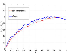
Depending on the underlying $\boldsymbol{\theta}$ and the noise realization $\mathbf{w}$, either the soft-thresholding estimator or the eBayes estimator may have the smaller loss. This is illustrated in Fig. 1, which compares the performance of the two estimators for two different kinds of $\boldsymbol{\theta}$ of length $n=1000$. The average normalized losses for the two cases are shown Figs. 1a and 1b as a function of the true sparsity level $\eta=\epsilon$, which is assumed to be known for both estimators. In the figures, the threshold $\lambda^{*}$ for $\hat{\boldsymbol{\theta}}_{ST}$ is chosen as [24, Sec. 3]

$$\lambda^{*} =\operatorname*{arg\,min}_{\lambda\geq 0}\left\{\epsilon(1+\lambda^{2})+(1-\epsilon)\left[2(1+\lambda^{2})\Phi(-\lambda)-2\lambda\phi(\lambda)\right]\right\},$$

where $\phi$ is the standard normal density, and $\Phi(x)\vcentcolon=\int_{-\infty}^{x}\phi(u)du$. This choice $\lambda^{*}$ minimizes the worst-case soft-thresholding risk over the class of all $\boldsymbol{\theta}$ with sparsity level $\epsilon$ [2].

The plots indicate that depending on the underlying $\boldsymbol{\theta}$, either $\hat{\boldsymbol{\theta}}_{ST}$ or $\hat{\boldsymbol{\theta}}_{EB}$ may have smaller loss. The goal is to construct an estimator that reliably chooses the estimator with lower loss. Noting that the loss depends on the underlying $\boldsymbol{\theta}$ as well as the noise realization, we propose a hybrid estimator that chooses one of the two competing estimators by comparing their Stein’s unbiased risk estimates (SURE) [25]. These risk estimates are given in Section 3. A key result of this paper is that for any $\boldsymbol{\theta}$, the loss of the hybrid estimator (which chooses one of the two estimators based on SURE) concentrates on the smaller of the two losses. In particular, the probability of the actual normalized loss deviating from the smaller one by more than $t$ decays exponentially in $n\min\{t,t^{2}\}$ for $t>0$.

The contributions of this paper are as follows:

• We derive the eBayes estimator in Sec. 2, and a risk function estimator based on Stein’s unbiased risk estimate (SURE) in Sec. 3.

• Sec. 4 contains the main theoretical results of the paper. The first result (Theorem 1) is a concentration inequality for the SURE of eBayes, which shows that for large $n$, the risk estimate concentrates on a deterministic value which is within $\mathcal{O}({1}/{\sqrt{n}})$ of the true risk. We remark that unlike the soft-thresholding estimator, the concentration of the SURE for eBayes cannot be established directly via readily available Gaussian concentration results as it does not satisfy Lipschitz or similar conditions.

  We then show in Theorem 2 that the loss of the eBayes estimator concentrates on a deterministic value that is within $\mathcal{O}({1}/{\sqrt{n}})$ of the eBayes risk. Theorem 4 shows that soft-thresholding loss concentrates on the true risk of soft-thresholding. Finally, we use the above concentration results to analyze the performance of a hybrid estimator which chooses the estimator (soft-thresholding or eBayes) with the smaller risk estimate. Theorem 5 shows that for the hybrid estimator, the loss concentrates on the minimum of the losses of the two rival estimators, and its risk is within $\mathcal{O}({1}/{\sqrt{n}})$ of the minimum of the two risks. Thus, the hybrid estimator uses the data to reliably choose an estimator tailored to the underlying $\boldsymbol{\theta}$.

• Sec. 5 provides simulation results to validate the theoretical results. The simulation results suggest that the proposed eBayes estimator is superior to soft-thresholding in a variety of cases, including the case where the non-zero entries come from a distribution with heavier-than-Gaussian tails, e.g., the Laplace distribution. In Sec. 5.1, we use the eBayes and the hybrid estimators as denoisers in the AMP algorithm for compressed sensing, and compare their performance with that of the soft-thresholding denoiser.

The approach taken in this paper of obtaining concentration inequalities for risk estimates can be used to bound the risk of a hybrid estimator that picks one among several estimators, provided one has concentration bounds for the risk estimates of each of the competing estimators. This suggests that an interesting direction for future work is to obtain concentration bounds for the risk estimates and loss functions of other useful estimators whose parameters depend on the data, e.g., an empirical Bayes estimator based on a Bernoulli-Laplace prior.

1.1 Related Work

In the context of wavelets, several works have considered estimators based on a signal prior that is a mixture of a point mass at $0$ and a Gaussian distribution, see e.g., [26, 27]. In most of these works, the hyperparameters of the prior are chosen based on some prior information about the signal. Martin and Walker [28] propose an estimator based on a data-dependent prior, and show that the resulting empirical Bayes estimator is asymptotically minimax. Johnstone and Silverman [4, 5] proposed empirical Bayes estimators based on a prior that is a mixture of a point mass at $0$ and a distribution with a heavy-tailed density. The weights of the mixture are first determined using marginal log-likelihood; the estimator then uses a thresholding rule based on the posterior median. It was shown that the risk of this estimator over the class of $\eta$-sparse vectors is within a constant factor of the minimax risk when the sparsity level $\eta$ is small enough.

In this paper, we fix the mixture weight for the eBayes estimator and then empirically estimate the location and scale parameters of the continuous part of the prior. This allows us to obtain concentration inequalities for the risk estimates, which then lead to concentration results for the loss and bounds for the risk for both the eBayes and the hybrid estimator.

Our previous work [29] also used concentration inequalities to characterize the performance of estimators with data-driven parameters. However, the estimators proposed in that paper were for general $\boldsymbol{\theta}$, as opposed to the sparse $\boldsymbol{\theta}$ considered here. Moreover, the loss function estimates in [29] are not based on SURE as the estimators are not smooth. Consequently, the techniques required to obtain the concentration results in [29] are quite different from those used here.

A recent paper by Zhang and Bhattacharya [30] also considers an empirical Bayes estimator defined via the prior in (1.5). The parameters of the prior are estimated by maximizing the marginal likelihood using the EM algorithm, and the properties of the posterior median and the posterior mean are studied. When the density $\psi$ in the prior is unimodal and satisfies certain conditions, it is shown in [30, Theorem 2.2] that the SURE corresponding to the posterior mean is within $\mathcal{O}(\frac{(\log n)^{3/2}}{\sqrt{n}})$ of the true risk with high probability. We comment on the differences between this result and our SURE concentration result (Theorem 1) in Note 1 on p.1.

As an alternative to using a hybrid estimator that picks one of several estimators based on risk estimates, George [31] and Leung and Barron [6, 7] have proposed combining the estimators using exponential mixture weights based on the risk estimates. We note that in high dimensions, the weight assigned to the estimator with the smallest risk estimate is exponentially larger (in $n$) than the others, so it is effectively equivalent to picking the estimator with the smallest risk estimate.

Notation: The set $\{1,2,\cdots,n\}$ is denoted by $[n]$. Bold lowercase (uppercase) letters are used to denote vectors (matrices), and plain lowercase letters for their entries. For example, the entries of $\mathbf{y}$ are $y_{i}$, $i=1,\cdots,n$. All vectors have length $n$ and are column vectors. The transpose of $\mathbf{y}$ is denoted by $\mathbf{y}^{T}$. The complement of an event $\mathcal{E}$ is denoted by $\mathcal{E}^{c}$, and its indicator function by $\mathsf{1}_{\{\mathcal{E}\}}$. For a random variable $X$, $X_{+}$ denotes $\max(0,X)$. For positive-valued functions $f(n)$ and $g(n)$, the notation $f(n)=\mathcal{O}(g(n))$ means that $\exists k>0$ such that $\forall n>n_{0}$, $f(n)\leq kg(n)$. Also, for a sequence of random variables $\{X_{n},n=1,2,\cdots\}$ and a sequence of deterministic numbers $\{a_{n},n=1,2,\cdots\}$, the notation $X_{n}=\mathcal{O}_{P}(a_{n})$ implies that for any $\delta>0$, there exists a finite $M>0$ and a finite $N>0$ such that $\mathbb{P}\left(|X_{n}/a_{n}|\geq M\right)\leq\delta$, $\forall n>N$.

2 Empirical Bayes Estimator

If the $\{\theta_{i}\},i\in[n]$ were generated i.i.d. according to the distribution $f(\theta;\epsilon,\mu,\xi)$ in (1.5), then the conditional mean of $\theta$ given $y$ is the optimal estimator for squared-error loss. The empirical Bayes estimator for a fixed $\epsilon\in[0,1]$ is this conditional mean, with the values of $\mu,\xi$ estimated from the data $\mathbf{y}$. Hence, $\forall i\in[n]$,

$$\hat{\boldsymbol{\theta}}_{EB,i}(\mathbf{y;\epsilon})=\frac{\int_{\mathbb{R}}xf(x;\epsilon,\hat{\mu},\hat{\xi})\phi(y_{i}-x)dx}{\int_{\mathbb{R}}f(x;\epsilon,\hat{\mu},\hat{\xi})\phi(y_{i}-x)dx}.$$ (2.1)

In (2.1), $\phi(x):=\frac{1}{\sqrt{2\pi}}e^{-x^{2}/2}$ is the standard normal density, and $\hat{\mu},\hat{\xi}$ are the estimates of $\mu,\xi$ from $\mathbf{y}$. A consistent estimator for the location parameter $\mu$ (converging in probability to $\mu$) is

$$\hat{\mu}(\mathbf{y})={\bar{y}}/{\epsilon},$$ (2.2)

where the empirical mean $\bar{y}=\sum_{i}y_{i}/n$. The scale parameter can be estimated using the second moment $\overline{y^{2}}:=\lVert\mathbf{y}\rVert^{2}/n$ and the mean $\bar{y}$. In this paper, we consider the Gaussian density for $\psi$ in (1.5) so that

$$\psi(\theta;\mu,\xi)=\frac{1}{\sqrt{2\pi\xi^{2}}}\exp(-(\theta-\mu)^{2}/2\xi^{2}).$$

The mean $\mu$ is estimated as in (2.2), and $\xi^{2}$, being the variance, is estimated as

$$\widehat{\xi^{2}}(\mathbf{y})=\frac{1}{\epsilon}\left(\overline{y^{2}}-\frac{(\bar{y})^{2}}{\epsilon}-1\right)_{+}.$$ (2.3)

The resulting empirical Bayes estimator is

$$\hat{\boldsymbol{\theta}}_{EB,i}(\mathbf{y;\epsilon})=\frac{\hat{\mu}+\left(1-\frac{1}{1+\widehat{\xi^{2}}}\right)(y_{i}-\hat{\mu})}{1+\frac{(1-\epsilon)}{\epsilon}\sqrt{1+\widehat{\xi^{2}}}\,\exp\left(-\frac{y_{i}^{2}}{2}+\frac{(y_{i}-\hat{\mu})^{2}}{2(1+\widehat{\xi^{2}})}\right)},\ i\in[n].$$ (2.4)

For $\epsilon=1$, $\hat{\boldsymbol{\theta}}_{EB}$ reduces to the positive-part Lindley’s estimator given in (1.4).

Note that $\hat{\boldsymbol{\theta}}_{EB}$ is a shrinkage estimator — the numerator shrinks each $y_{i}$ towards a common element $\hat{\mu}$. There are two terms that determine the overall shrinkage, the first being the term $\left[1-\frac{1}{1+\widehat{\xi^{2}}}\right]$ which is common for all the $y_{i}$. The second term influencing the shrinkage is the exponential in the denominator which depends on $y_{i}$. To get intuition about the role of these terms, assume that the location parameter is zero, i.e., $\hat{\mu}=0$ in (2.4). Then the estimator is given by

$$\hat{\boldsymbol{\theta}}_{EB,i}(\mathbf{y};\epsilon)=\frac{\left(\frac{\widehat{\xi^{2}}}{1+\widehat{\xi^{2}}}\right)y_{i}}{1+\frac{(1-\epsilon)}{\epsilon}\sqrt{1+\widehat{\xi^{2}}}\exp\left(-\frac{\widehat{\xi^{2}}y_{i}^{2}}{2(1+\widehat{\xi^{2}})}\right)}$$ (2.5)

with $\widehat{\xi^{2}}=(1/\epsilon)(\overline{y^{2}}-1)_{+}$. When the magnitude of $\theta_{i}$ is large ($\gg 1$), $y_{i}$ is likely to have large magnitude as well; hence, the amount of shrinkage due to the denominator is smaller. On the other hand, for $\theta_{i}$ with smaller magnitude, $y_{i}$ is also likelier to have smaller magnitude and the amount of shrinkage is correspondingly larger.

To further understand the role of the shrinkage factor in the numerator, suppose that an oracle provided us with the values $\{\theta_{i}^{2}\},i\in[n]$. Then, the ideal linear minimax estimator is [32]

$$\hat{\theta}_{i}=\frac{\theta_{i}^{2}}{(1+\theta_{i}^{2})}y_{i},~{}~{}~{}~{}i\in[n].$$

Noting that $\lVert\boldsymbol{\theta}\rVert^{2}/(n\epsilon)$ is the mean of the $\{\theta_{i}^{2}\}$ for $\theta_{i}\neq 0$, in the absence of the oracle, the estimator attempts to approximate the term ${\theta_{i}^{2}}/{(1+\theta_{i}^{2})}$ via the ratio $\frac{\lVert\boldsymbol{\theta}\rVert^{2}/(n\epsilon)}{1+\lVert\boldsymbol{\theta}\rVert^{2}/(n\epsilon)}$. This ratio in turn is well-approximated for large $n$ by $\widehat{\xi^{2}}/(1+\widehat{\xi^{2}})$ — this can be seen from (2.3) by observing that $\overline{y^{2}}=\lVert\mathbf{y}\rVert^{2}/n$ is close to its mean $\lVert\boldsymbol{\theta}\rVert^{2}/n+1$ (when $\bar{y}=0$). This is the significance of the common shrinkage factor in the numerator. The denominator further shrinks the estimate if it believes that the $\theta_{i}$ has a small magnitude.

To summarize, in (2.5), the $y_{i}$ corresponding to the large non-zero components of $\boldsymbol{\theta}$ are shrunk by approximately $\frac{\lVert\boldsymbol{\theta}\rVert^{2}/(n\epsilon)}{1+\lVert\boldsymbol{\theta}\rVert^{2}/(n\epsilon)}$, while those corresponding to the zero components of $\boldsymbol{\theta}$ are made even closer to $0$.

3 Risk Estimates and the Hybrid Estimator

Recall from Fig. 1 that depending on the underlying $\boldsymbol{\theta}$, either $\hat{\boldsymbol{\theta}}_{ST}$ or $\hat{\boldsymbol{\theta}}_{EB}$ may have smaller loss. To construct a hybrid estimator that reliably chooses the better estimator, we use Stein’s unbiased risk estimate (SURE) [25] to estimate the losses of each estimator.

Fact 1.

[25] If an estimator $\hat{\boldsymbol{\theta}}(\mathbf{y})$ is almost everywhere differentiable, then

$$\hat{R}(\boldsymbol{\theta},\hat{\boldsymbol{\theta}}(\mathbf{y}))\vcentcolon=-n+\lVert\mathbf{y}-\hat{\boldsymbol{\theta}}\rVert^{2}+2\sum_{i=1}^{n}\frac{\partial\hat{\theta}_{i}}{\partial y_{i}}$$

is an unbiased estimate of the risk $R(\boldsymbol{\theta},\hat{\boldsymbol{\theta}})$, i.e., $\mathbb{E}\left[\hat{R}(\boldsymbol{\theta},\hat{\boldsymbol{\theta}}(\mathbf{y}))\right]=R(\boldsymbol{\theta},\hat{\boldsymbol{\theta}})$ where the expectation is again over $\mathbf{y}\sim\mathcal{N}(\boldsymbol{\theta},\mathbf{I})$. $\hat{R}(\boldsymbol{\theta},\hat{\boldsymbol{\theta}}(\mathbf{y}))$ is called the SURE of $\hat{\boldsymbol{\theta}}$.

Using SURE, the normalized risk estimate for $\hat{\boldsymbol{\theta}}_{ST}$ with threshold $\lambda$ is given by

$$\hat{R}(\boldsymbol{\theta},\hat{\boldsymbol{\theta}}_{ST};\lambda)=-1+\frac{\lVert\mathbf{y}-\hat{\boldsymbol{\theta}}_{ST}\rVert^{2}}{n}+\frac{2}{n}\sum_{i=1}^{n}\mathsf{1}_{\{y_{i}^{2}>\lambda^{2}\}}.$$ (3.1)

To keep the exposition simple, for our concentration results we assume that the location parameter $\hat{\mu}$ in $\hat{\boldsymbol{\theta}}_{EB}$ is zero, so that $\hat{\boldsymbol{\theta}}_{EB}$ is given by (2.5). Extending the results to the case with a general $\hat{\mu}$ is straightforward, though a bit cumbersome. Let

$$\begin{split}a_{\mathbf{y}}\vcentcolon&=\frac{\widehat{\xi}^{2}}{1+\widehat{\xi}^{2}}=\left[1-\frac{\epsilon}{(\lVert\mathbf{y}\rVert^{2}/n-1)_{+}+\epsilon}\right],\\ d_{\mathbf{y}}\vcentcolon&=1+\widehat{\xi}^{2}=1+\frac{1}{\epsilon}\left(\frac{\lVert\mathbf{y}\rVert^{2}}{n}-1\right)_{+},\\ c_{\mathbf{y}}\vcentcolon&=\frac{1-\epsilon}{\epsilon}\sqrt{1+\widehat{\xi}^{2}}=\frac{1-\epsilon}{\epsilon}\sqrt{d_{\mathbf{y}}},\\ b_{i}(\mathbf{y})\vcentcolon&=1+c_{\mathbf{y}}e^{-\frac{a_{\mathbf{y}}y_{i}^{2}}{2}}.\end{split}$$ (3.2)

Using SURE, the normalized risk estimate for $\hat{\boldsymbol{\theta}}_{EB}$ with $\hat{\mu}=0$ is

$$\frac{\hat{R}(\boldsymbol{\theta},\hat{\boldsymbol{\theta}}_{EB}(\mathbf{y});\epsilon)}{n}=-1+\frac{1}{n}\lVert\mathbf{y}-\hat{\boldsymbol{\theta}}_{EB}\rVert^{2}+\frac{2}{n}\sum_{i=1}^{n}\frac{\partial\hat{\theta}_{i}}{\partial y_{i}}$$

$$=-1+\frac{\lVert\mathbf{y}\rVert^{2}}{n}+\frac{a^{2}_{\mathbf{y}}}{n}\sum_{i=1}^{n}\frac{y_{i}^{2}}{b^{2}_{i}(\mathbf{y})}-\frac{2a_{\mathbf{y}}}{n}\sum_{i=1}^{n}\frac{y_{i}^{2}}{b_{i}(\mathbf{y})}$$

$$\quad+\frac{2}{n}\sum_{i=1}^{n}\left[\frac{a_{\mathbf{y}}}{b_{i}(\mathbf{y})}+\frac{a_{\mathbf{y}}^{\prime}(i)y_{i}}{b_{i}(\mathbf{y})}+\frac{\left[a_{\mathbf{y}}^{\prime}(i)c_{\mathbf{y}}(y_{i}^{2}/2)+a_{\mathbf{y}}c_{\mathbf{y}}y_{i}-c_{\mathbf{y}}^{\prime}(i)\right]a_{\mathbf{y}}y_{i}e^{-\frac{a_{\mathbf{y}}y_{i}^{2}}{2}}}{b_{i}^{2}(\mathbf{y})}\right]$$

$$=\left(\frac{\lVert\mathbf{y}\rVert^{2}}{n}-1\right)+\frac{a^{2}_{\mathbf{y}}}{n}\sum_{i=1}^{n}\frac{y_{i}^{2}}{b^{2}_{i}(\mathbf{y})}-\frac{2a_{\mathbf{y}}}{n}\sum_{i=1}^{n}\frac{y_{i}^{2}}{b_{i}(\mathbf{y})}$$

$$\quad+\frac{2}{n}\sum_{i=1}^{n}\left[\frac{a_{\mathbf{y}}}{b_{i}(\mathbf{y})}+\frac{2y_{i}^{2}}{n\epsilon d_{\mathbf{y}}^{2}b_{i}(\mathbf{y})}\mathsf{1}_{\{\lVert\mathbf{y}\rVert^{2}>n\}}+\left(\frac{(1-\epsilon)a_{\mathbf{y}}}{n\epsilon^{2}d_{\mathbf{y}}^{3/2}}\right)\frac{y_{i}^{4}e^{-\frac{a_{\mathbf{y}}y_{i}^{2}}{2}}}{b_{i}^{2}(\mathbf{y})}\right]$$

$$\quad+\frac{2}{n}\sum_{i=1}^{n}\left[\frac{a_{\mathbf{y}}^{2}c_{\mathbf{y}}y_{i}^{2}e^{-\frac{a_{\mathbf{y}}y_{i}^{2}}{2}}}{b_{i}^{2}(\mathbf{y})}-\left(\frac{(1-\epsilon)a_{\mathbf{y}}}{\epsilon^{2}\sqrt{d_{\mathbf{y}}}}\right)\frac{y_{i}^{2}e^{-\frac{a_{\mathbf{y}}y_{i}^{2}}{2}}}{nb_{i}^{2}(\mathbf{y})}\right]$$

where $a_{\mathbf{y}}^{\prime}(i)=\frac{\partial a_{\mathbf{y}}}{\partial y_{i}}$, $c_{\mathbf{y}}^{\prime}(i)=\frac{\partial c_{\mathbf{y}}}{\partial y_{i}}$. Rearranging terms and simplifying, we obtain

$$\begin{split}&\frac{\hat{R}(\boldsymbol{\theta},\hat{\boldsymbol{\theta}}_{EB}(\mathbf{y});\epsilon)}{n}=\left(\frac{\lVert\mathbf{y}\rVert^{2}}{n}-1\right)+\frac{a^{2}_{\mathbf{y}}}{n}\sum_{i=1}^{n}\frac{y_{i}^{2}\big{(}1+2c_{\mathbf{y}}e^{-\frac{a_{\mathbf{y}}y_{i}^{2}}{2}}\big{)}}{b^{2}_{i}(\mathbf{y})}-\frac{2a_{\mathbf{y}}}{n}\sum_{i=1}^{n}\frac{y_{i}^{2}-1}{b_{i}(\mathbf{y})}\\ &+\frac{4}{d_{\mathbf{y}}^{2}\epsilon n^{2}}\sum_{i=1}^{n}\frac{y_{i}^{2}}{b_{i}(\mathbf{y})}\mathsf{1}_{\{\lVert\mathbf{y}\rVert^{2}>n\}}+\frac{2(1-\epsilon)a_{\mathbf{y}}}{d_{\mathbf{y}}^{3/2}\epsilon^{2}n^{2}}\sum_{i=1}^{n}\frac{y_{i}^{4}e^{-\frac{a_{\mathbf{y}}y_{i}^{2}}{2}}}{b_{i}^{2}(\mathbf{y})}-\frac{2(1-\epsilon)a_{\mathbf{y}}}{\sqrt{d_{\mathbf{y}}}\epsilon^{2}n^{2}}\sum_{i=1}^{n}\frac{y_{i}^{2}e^{-\frac{a_{\mathbf{y}}y_{i}^{2}}{2}}}{b_{i}^{2}(\mathbf{y})}.\end{split}$$ (3.3)

For large $n$, the last three terms of (3.3) with $n^{2}$ in the denominator are very small and can be neglected in a practical application of the risk estimate. More precisely, the proof of Theorem 1 in the next section shows that the last three terms concentrate around deterministic constants of order $\frac{1}{n}$.

We use the risk estimates in (3.1) and (3.2) to define a hybrid estimator that aims to select the estimator with smaller loss for the $\boldsymbol{\theta}$ in context. The hybrid estimator is defined as

$$\hat{\boldsymbol{\theta}}_{H} =\gamma_{\mathbf{y}}\hat{\boldsymbol{\theta}}_{EB}+(1-\gamma_{\mathbf{y}})\hat{\boldsymbol{\theta}}_{ST},$$ (3.4)

$$\gamma_{\mathbf{y}} =\left\{\begin{array}[]{ccc}1&\textrm{if }&\hat{R}(\boldsymbol{\theta},\hat{\boldsymbol{\theta}}_{EB}(\mathbf{y}))\leq\hat{R}(\boldsymbol{\theta},\hat{\boldsymbol{\theta}}_{ST}(\mathbf{y})),\\ 0&\textrm{otherwise.}&\\ \end{array}\right.$$ (3.7)

In the next section, we obtain concentration results for the risk estimates and loss functions of $\hat{\boldsymbol{\theta}}_{ST}$ and $\hat{\boldsymbol{\theta}}_{EB}$, and use these to show that the loss of the hybrid estimator concentrates on the minimum of the losses of the two estimators.

4 Main Results

4.1 Concentration Results for the Empirical Bayes Estimator

The constants in our concentration results for the eBayes estimator depend on $\boldsymbol{\theta}$ via $\frac{1}{n}\sum_{i=1}^{n}\theta_{i}^{4}$. In order to make these constants universal, we assume that the fourth moment of $\boldsymbol{\theta}$ is bounded.

Assumption A: There exists a finite constant $\Lambda>0$ such that $\frac{1}{n}\sum_{i=1}^{n}\theta_{i}^{4}\leq\Lambda$.

When Assumption A is satisfied, the constants in the concentration results depend only on $\Lambda$ (and not on the underlying $\boldsymbol{\theta}$ or $n)$. For brevity, we henceforth do not explicitly indicate the dependence on $\lambda$ and $\epsilon$ in the notation for the risk estimates on the LHS of (3.1) and (3.3), respectively.

Theorem 1.

Consider a sequence of $\boldsymbol{\theta}$ with increasing dimension $n$ and satisfying Assumption A. Then the risk estimate $\hat{R}(\boldsymbol{\theta},\hat{\boldsymbol{\theta}}_{EB}(\mathbf{y}))$ satisfies the following for any $t>0$:

$$\mathbb{P}\left(\frac{1}{n}\left|\hat{R}(\boldsymbol{\theta},\hat{\boldsymbol{\theta}}_{EB}(\mathbf{y}))-R_{1}(\boldsymbol{\theta},\hat{\boldsymbol{\theta}}_{EB})\right|\geq t\right)\leq Ke^{-nk\min(t,t^{2})}$$ (4.1)

where $0<K\leq 24$ and $k>0$ are absolute constants, and $R_{1}(\boldsymbol{\theta},\hat{\boldsymbol{\theta}}_{EB})$ is a deterministic quantity such that

$$\left|\frac{R_{1}(\boldsymbol{\theta},\hat{\boldsymbol{\theta}}_{EB})}{n}-\frac{{R}(\boldsymbol{\theta},\hat{\boldsymbol{\theta}}_{EB})}{n}\right|=\mathcal{O}\left(\frac{1}{\sqrt{n}}\right).$$ (4.2)

Proof.

The $i^{th}$ element of $\hat{\boldsymbol{\theta}}_{EB}$ in (2.5) is $\hat{\theta}_{i}=\frac{a_{\mathbf{y}}y_{i}}{b_{i}(\mathbf{y})}$. The SURE of $\hat{\boldsymbol{\theta}}_{EB}$ is as given in (3.3). We need to show concentration for each term on the RHS of (3.3). In the following, $K,k,k_{0},\ldots,k_{10}$ are universal positive constants that do not depend on $t$ or $n$.

Since $\lVert\mathbf{y}\rVert^{2}$ is a non-central chi-squared random variable with mean $\lVert\boldsymbol{\theta}\rVert^{2}+n$, we have the following large deviations bound [33]. For any $t>0$

$$\mathbb{P}\left(\left|\frac{\lVert\mathbf{y}\rVert^{2}}{n}-1-\frac{\lVert\boldsymbol{\theta}\rVert^{2}}{n}\right|\geq t\right)\leq 2e^{-nk_{0}\min(t,t^{2})}.$$ (4.3)

The concentration for the remaining terms of (3.3) is shown using two lemmas stated below. The proofs of the lemmas are given Sec. 6.2. The first lemma shows that the last three terms in (3.3) concentrate around their expectations.

Lemma 4.1.

Let

$$u_{n}\vcentcolon=\frac{4}{\epsilon d_{\mathbf{y}}^{2}n^{2}}\sum_{i=1}^{n}\frac{y_{i}^{2}}{b_{i}(\mathbf{y})}\mathsf{1}_{\{\lVert\mathbf{y}\rVert^{2}>n\}},v_{n}\vcentcolon=\frac{2(1-\epsilon)a_{\mathbf{y}}}{d_{\mathbf{y}}^{3/2}n^{2}\epsilon^{2}}\sum_{i=1}^{n}\frac{y_{i}^{4}e^{-\frac{a_{\mathbf{y}}y_{i}^{2}}{2}}}{b_{i}^{2}(\mathbf{y})},x_{n}\vcentcolon=\frac{2(1-\epsilon)a_{\mathbf{y}}}{n^{2}\epsilon^{2}\sqrt{d_{\mathbf{y}}}}\sum_{i=1}^{n}\frac{y_{i}^{2}e^{-\frac{a_{\mathbf{y}}y_{i}^{2}}{2}}}{b_{i}^{2}(\mathbf{y})}.$$

Then for any $t>0$,

$$\begin{split}\mathbb{P}\left(|u_{n}-\mathbb{E}u_{n}|\geq t\right)&\leq 2e^{-n^{2}k_{1}t^{2}},\qquad\mathbb{P}\left(|v_{n}-\mathbb{E}v_{n}|\geq t\right)\leq 2e^{-n^{2}k_{2}t^{2}},\\ \mathbb{P}\left(|x_{n}-\mathbb{E}x_{n}|\geq t\right)&\leq 2e^{-n^{2}k_{3}t^{2}}.\end{split}$$ (4.4)

Establishing concentration inequalities for the second and third terms of (3.3) around their respective means is more challenging. This is because the summands are dependent random variables and it is not straightforward to prove that their sum satisfies Lipschitz or similar conditions for which Gaussian concentration results are readily available. Hence, in the following lemma, we prove concentration of these terms around certain deterministic values, and then show that these deterministic values are close to the required means.

Lemma 4.2.

Let

$$\begin{split}f_{n}\vcentcolon=&\frac{a^{2}_{\mathbf{y}}}{n}\sum_{i=1}^{n}\frac{y_{i}^{2}}{b^{2}_{i}(\mathbf{y})}-\frac{a^{2}}{n}\sum_{i=1}^{n}\mathbb{E}\left[\frac{y_{i}^{2}}{\left(1+ce^{-ay_{i}^{2}/2}\right)^{2}}\right],\\ g_{n}\vcentcolon=&\frac{2a_{\mathbf{y}}}{n}\sum_{i=1}^{n}\frac{y_{i}^{2}}{b_{i}(\mathbf{y})}-\frac{2a}{n}\sum_{i=1}^{n}\mathbb{E}\left[\frac{y_{i}^{2}}{1+ce^{-ay_{i}^{2}/2}}\right],\\ h_{n}\vcentcolon=&\frac{2a_{\mathbf{y}}}{n}\sum_{i=1}^{n}\frac{1}{b_{i}(\mathbf{y})}-\frac{2a}{n}\sum_{i=1}^{n}\mathbb{E}\left[\frac{1}{1+ce^{-ay_{i}^{2}/2}}\right],\\ w_{n}\vcentcolon=&\frac{2a_{\mathbf{y}}^{2}c_{\mathbf{y}}}{n}\sum_{i=1}^{n}\frac{y_{i}^{2}e^{-\frac{a_{\mathbf{y}}y_{i}^{2}}{2}}}{b_{i}^{2}(\mathbf{y})}-\frac{2a^{2}c}{n}\sum_{i=1}^{n}\mathbb{E}\left[\frac{y_{i}^{2}e^{-\frac{ay_{i}^{2}}{2}}}{\left(1+ce^{-ay_{i}^{2}/2}\right)^{2}}\right],\end{split}$$

where

$$a\vcentcolon=\frac{\lVert\boldsymbol{\theta}\rVert^{2}/n}{\epsilon+\lVert\boldsymbol{\theta}\rVert^{2}/n},\quad c\vcentcolon=\frac{1-\epsilon}{\epsilon^{3/2}}\sqrt{\epsilon+\lVert\boldsymbol{\theta}\rVert^{2}/n}.$$ (4.5)

Then, for any $t>0$,

$$\mathbb{P}\left(\left|f_{n}\right|\geq t\right) \leq 4e^{-nk_{4}\min(t,t^{2})},$$ (4.6)

$$\mathbb{P}\left(|g_{n}|\geq t\right) \leq 4e^{-nk_{5}\min(t,t^{2})},$$ (4.7)

$$\mathbb{P}\left(|h_{n}|\geq t\right) \leq 4e^{-nk_{6}\min(t,t^{2})},$$ (4.8)

$$\mathbb{P}\left(|w_{n}|\geq t\right) \leq 4e^{-nk_{7}\min(t,t^{2})}.$$ (4.9)

Using the results of Lemmas 4.1 and 4.2, we obtain, for any $t>0$,

$$\mathbb{P}\left(\left|\frac{\hat{R}(\boldsymbol{\theta},\hat{\boldsymbol{\theta}}_{EB}(\mathbf{y}))}{n}-\frac{R_{1}(\boldsymbol{\theta},\hat{\boldsymbol{\theta}}_{EB})}{n}\right|\geq t\right)\leq 24e^{-nk\min(t,t^{2})}$$

where $k$ is an absolute positive constant and

$$\frac{R_{1}(\boldsymbol{\theta},\hat{\boldsymbol{\theta}}_{EB})}{n}$$

$$=b+\frac{a^{2}}{n}\sum_{i=1}^{n}\mathbb{E}\left[\frac{y_{i}^{2}}{\left(1+ce^{-ay_{i}^{2}/2}\right)^{2}}\right]-\frac{2a}{n}\sum_{i=1}^{n}\mathbb{E}\left[\frac{y_{i}^{2}-1}{1+ce^{-ay_{i}^{2}/2}}\right]+\frac{2a^{2}c}{n}\sum_{i=1}^{n}\mathbb{E}\left[\frac{y_{i}^{2}e^{-\frac{ay_{i}^{2}}{2}}}{\left(1+ce^{-ay_{i}^{2}/2}\right)^{2}}\right]$$

$$+\frac{4}{\epsilon n^{2}}\sum_{i=1}^{n}\mathbb{E}\left[\frac{y_{i}^{2}}{d_{\mathbf{y}}^{2}b_{i}(\mathbf{y})}\mathsf{1}_{\{\lVert\mathbf{y}\rVert^{2}>n\}}\right]+\frac{2(1-\epsilon)}{n^{2}\epsilon^{2}}\sum_{i=1}^{n}\mathbb{E}\left[\frac{a_{\mathbf{y}}y_{i}^{4}e^{-\frac{a_{\mathbf{y}}y_{i}^{2}}{2}}}{d_{\mathbf{y}}^{3/2}b_{i}^{2}(\mathbf{y})}\right]-\frac{2(1-\epsilon)}{n^{2}\epsilon^{2}}\sum_{i=1}^{n}\mathbb{E}\left[\frac{a_{\mathbf{y}}y_{i}^{2}e^{-\frac{a_{\mathbf{y}}y_{i}^{2}}{2}}}{\sqrt{d_{\mathbf{y}}}b_{i}^{2}(\mathbf{y})}\right],$$

with the constants $a,c$ as defined in (4.5).

Finally, to prove (4.2), we use Lemma 6.8 to get

$$\mathbb{E}\left|\frac{\hat{R}(\boldsymbol{\theta},\hat{\boldsymbol{\theta}}_{EB}(\mathbf{y}))}{n}-\frac{R_{1}(\boldsymbol{\theta},\hat{\boldsymbol{\theta}}_{EB})}{n}\right|\leq\frac{C}{\sqrt{n}}\left(1+\frac{1}{\sqrt{n}}\right)$$ (4.10)

for some positive constant $C$. Since $\mathbb{E}|X|\geq|\mathbb{E}X|$ and $\mathbb{E}\left[\hat{R}(\boldsymbol{\theta},\hat{\boldsymbol{\theta}}_{EB}(\mathbf{y}))\right]={R}(\boldsymbol{\theta},\hat{\boldsymbol{\theta}}_{EB})$, (4.2) follows.

∎

Note 1.

Theorem 1 implies that $\frac{1}{n}\left[\hat{R}(\boldsymbol{\theta},\hat{\boldsymbol{\theta}}_{EB}(\mathbf{y}))-R(\boldsymbol{\theta},\hat{\boldsymbol{\theta}}_{EB})\right]=\mathcal{O}_{P}\left(\frac{1}{\sqrt{n}}\right)$. This is a slightly stronger result than [30, Theorem 2.2] which states that $\frac{1}{n}\left[\hat{R}(\boldsymbol{\theta},\hat{\boldsymbol{\theta}}_{EB}(\mathbf{y}))-R(\boldsymbol{\theta},\hat{\boldsymbol{\theta}}_{EB})\right]=\mathcal{O}_{P}\left(\frac{(\log n)^{3/2}}{\sqrt{n}}\right)$. The result in [30, Theorem 2.2] applies to a class of densities $\psi$ in (1.5) that are unimodal with $\log\psi$ satisfying certain Lipschitz conditions. Though this class is more general than the Gaussian, the result is derived assuming that the parameters defining $\psi$ are fixed and do not depend on the data. (In particular, the parameters can take on any fixed value in a specified range which grows logarithmically with $n$.) In contrast, our parameter estimates $\hat{\mu}(\mathbf{y})$ and $\widehat{\xi^{2}}(\mathbf{y})$ depend on the data. Obtaining concentration results for terms with these data-dependent parameters (e.g., those in Lemma 4.2) is the key technical challenge in proving Theorem 1.

The next result shows that the normalized loss of the eBayes estimator concentrates on a deterministic value close to the true risk.

Theorem 2.

Consider a sequence of $\boldsymbol{\theta}$ with increasing dimension $n$ and satisfying Assumption A. Then the loss function $L(\boldsymbol{\theta},\hat{\boldsymbol{\theta}}_{EB})=\lVert\boldsymbol{\theta}-\hat{\boldsymbol{\theta}}_{EB}\rVert^{2}$ satisfies the following for any $t>0$:

$$\mathbb{P}\left(\frac{1}{n}\left|L(\boldsymbol{\theta},\hat{\boldsymbol{\theta}}_{EB}(\mathbf{y}))-R_{2}(\boldsymbol{\theta},\hat{\boldsymbol{\theta}}_{EB})\right|\geq t\right)\leq Ke^{-nk\min(t,t^{2})}$$ (4.11)

where $K\leq 10$ and $k$ are absolute positive constants, and $R_{2}(\boldsymbol{\theta},\hat{\boldsymbol{\theta}}_{EB})$ is a deterministic quantity such that

$$\left|\frac{R_{2}(\boldsymbol{\theta},\hat{\boldsymbol{\theta}}_{EB})}{n}-\frac{{R}(\boldsymbol{\theta},\hat{\boldsymbol{\theta}}_{EB})}{n}\right|=\mathcal{O}\left(\frac{1}{\sqrt{n}}\right).$$ (4.12)

Proof.

We have

$$\frac{L(\boldsymbol{\theta},\hat{\boldsymbol{\theta}}_{EB}(\mathbf{y}))}{n}=\frac{\lVert\boldsymbol{\theta}-\hat{\boldsymbol{\theta}}_{EB}\rVert^{2}}{n}=\frac{\lVert\boldsymbol{\theta}\rVert^{2}}{n}+\frac{\lVert\hat{\boldsymbol{\theta}}_{EB}(\mathbf{y})\rVert^{2}}{n}-\frac{2a_{\mathbf{y}}}{n}\sum_{i=1}^{n}\frac{\theta_{i}y_{i}}{b_{i}(\mathbf{y})}.$$ (4.13)

We have already shown in (4.6) that

$$\frac{\lVert\hat{\boldsymbol{\theta}}_{EB}(\mathbf{y})\rVert^{2}}{n}=\frac{a^{2}_{\mathbf{y}}}{n}\sum_{i=1}^{n}\frac{y_{i}^{2}}{b^{2}_{i}(\mathbf{y})}$$

concentrates around $\frac{a^{2}}{n}\sum_{i=1}^{n}\mathbb{E}\left[y_{i}^{2}/{(1+ce^{-ay_{i}^{2}/2})^{2}}\right]$. The concentration for the last term in (4.13) around its mean is complicated to prove due to the absence of any Lipschitz behaviour. We instead show in Sec. 6.3 that for any $t>0$,

$$\mathbb{P}\left(\frac{1}{n}\left|\sum_{i=1}^{n}\frac{\theta_{i}a_{\mathbf{y}}y_{i}}{b_{i}(\mathbf{y})}-\sum_{i=1}^{n}\mathbb{E}\left[\frac{a\theta_{i}y_{i}}{1+ce^{-ay_{i}^{2}/2}}\right]\right|\geq t\right)\leq 6e^{-nk\min(t,t^{2})}.$$ (4.14)

Thus, using the concentration inequalities in (4.6) and (4.14), from (4.13) we obtain that for any $t>0$,

$$\mathbb{P}\left(\left|\frac{L(\boldsymbol{\theta},\hat{\boldsymbol{\theta}}_{EB}(\mathbf{y}))}{n}-\frac{R_{2}(\boldsymbol{\theta},\hat{\boldsymbol{\theta}}_{EB})}{n}\right|\geq t\right)\leq 10e^{-nk\min(t,t^{2})}$$

where

$$\frac{R_{2}(\boldsymbol{\theta},\hat{\boldsymbol{\theta}}_{EB})}{n}=\frac{\lVert\boldsymbol{\theta}\rVert^{2}}{n}+\frac{a^{2}}{n}\sum_{i=1}^{n}\mathbb{E}\left[\frac{y_{i}^{2}}{\left(1+ce^{-ay_{i}^{2}/2}\right)^{2}}\right]-\frac{2a}{n}\sum_{i=1}^{n}\mathbb{E}\left[\frac{\theta_{i}y_{i}}{1+ce^{-ay_{i}^{2}/2}}\right]$$ (4.15)

with the constants $a,c$ as defined in (4.5). We note that due to Assumption A, the RHS of (4.15) is bounded by a universal constant not depending on $n$.

To prove (4.12), we apply Lemma 6.8 which shows that the concentration result (4.11) implies the following bound on the expected value:

$$\mathbb{E}\left|\frac{L(\boldsymbol{\theta},\hat{\boldsymbol{\theta}}_{EB}(\mathbf{y}))}{n}-\frac{R_{2}(\boldsymbol{\theta},\hat{\boldsymbol{\theta}}_{EB})}{n}\right|\leq\frac{C}{\sqrt{n}}\left(1+\frac{1}{\sqrt{n}}\right)$$ (4.16)

where $C$ is a universal positive constant. Since $\mathbb{E}|X|\geq|\mathbb{E}X|$ and $\mathbb{E}\left[L(\boldsymbol{\theta},\hat{\boldsymbol{\theta}}_{EB}(\mathbf{y}))\right]={R}(\boldsymbol{\theta},\hat{\boldsymbol{\theta}}_{EB})$, (4.12) follows.

∎

4.2 Concentration Results for the Soft-Thresholding Estimator

The concentration result for the risk estimate of soft-thresholding was obtained by Donoho and Johnstone [3]. In contrast to the eBayes estimator, the normalized risk estimate for soft-thresholding given in (3.1) is bounded. Therefore a concentration result can be directly obtained using Hoeffding’s inequality [34].

Theorem 3.

[3] The risk estimate $\hat{R}(\boldsymbol{\theta},\hat{\boldsymbol{\theta}}_{ST})$ for the soft-thresholding estimator satisfies the following for any $t>0$,

$$\mathbb{P}\left(\frac{1}{n}\left|\hat{R}(\boldsymbol{\theta},\hat{\boldsymbol{\theta}}_{ST}(\mathbf{y}))-{R}(\boldsymbol{\theta},\hat{\boldsymbol{\theta}}_{ST})\right|\geq t\right)\leq 2e^{-\frac{2t^{2}}{9(1+\lambda^{2})^{2}}}.$$ (4.17)

We can also show that the normalized loss of the soft-thresholding estimator concentrates on the true risk.

Theorem 4.

The loss function $L(\boldsymbol{\theta},\hat{\boldsymbol{\theta}}_{ST})=\lVert\boldsymbol{\theta}-\hat{\boldsymbol{\theta}}_{ST}\rVert^{2}$ of the soft-thresholding estimator satisfies the following for any $t>0$:

$$\mathbb{P}\left(\frac{1}{n}\left|L(\boldsymbol{\theta},\hat{\boldsymbol{\theta}}_{ST}(\mathbf{y}))-{R}(\boldsymbol{\theta},\hat{\boldsymbol{\theta}}_{ST})\right|\geq t\right)\leq 2e^{-nk\min(t,t^{2})}$$ (4.18)

where $k$ is an absolute positive constant.

Proof.

See Sec. 6.4. ∎

4.3 Concentration and Risk Bound for the Hybrid Estimator

For a given $\boldsymbol{\theta}$, let

$$L_{min}(\boldsymbol{\theta},\mathbf{y})\vcentcolon=\min\left\{L(\boldsymbol{\theta},\hat{\boldsymbol{\theta}}_{EB}(\mathbf{y})),L(\boldsymbol{\theta},\hat{\boldsymbol{\theta}}_{ST}(\mathbf{y}))\right\},$$

$$L_{max}(\boldsymbol{\theta},\mathbf{y})\vcentcolon=\max\left\{L(\boldsymbol{\theta},\hat{\boldsymbol{\theta}}_{EB}(\mathbf{y})),L(\boldsymbol{\theta},\hat{\boldsymbol{\theta}}_{ST}(\mathbf{y}))\right\},$$

$$L_{sep}(\boldsymbol{\theta},\mathbf{y})\vcentcolon=L_{max}(\boldsymbol{\theta},\mathbf{y})-L_{min}(\boldsymbol{\theta},\mathbf{y}),$$ (4.19)

$$\kappa_{n}\vcentcolon=\frac{\left|R_{1}(\boldsymbol{\theta},\hat{\boldsymbol{\theta}}_{EB})-R_{2}(\boldsymbol{\theta},\hat{\boldsymbol{\theta}}_{EB})\right|}{n},$$ (4.20)

where $R_{1}(\boldsymbol{\theta},\hat{\boldsymbol{\theta}}_{EB})$ and $R_{2}(\boldsymbol{\theta},\hat{\boldsymbol{\theta}}_{EB})$ are the deterministic concentrating values in Theorems 1 and 2, respectively. Note that $\kappa_{n}$ is an $\mathcal{O}(1/\sqrt{n})$ quantity since both $R_{1}(\boldsymbol{\theta},\hat{\boldsymbol{\theta}}_{EB})/n$ and $R_{2}(\boldsymbol{\theta},\hat{\boldsymbol{\theta}}_{EB})/n$ are within $\mathcal{O}(1/\sqrt{n})$ from ${R}(\boldsymbol{\theta},\hat{\boldsymbol{\theta}}_{EB})/n$. The following theorem characterizes the loss $L(\boldsymbol{\theta},\hat{\boldsymbol{\theta}}_{H}(\mathbf{y}))$ and the risk $R(\boldsymbol{\theta},\hat{\boldsymbol{\theta}}_{H})$ of the hybrid estimator.

Theorem 5.

Consider a sequence of $\boldsymbol{\theta}$ with increasing dimension $n$ and satisfying Assumption A. Then, for any $t>0$, we have

$$\mathbb{P}\left(\frac{1}{n}L(\boldsymbol{\theta},\hat{\boldsymbol{\theta}}_{H}(\mathbf{y}))\geq\frac{1}{n}L_{min}(\boldsymbol{\theta},\mathbf{y})+t+\kappa_{n}\right)\leq Ke^{-nk\min(t,t^{2})},$$ (4.21)

for some absolute positive constants $K$ and $k$. The risk of the hybrid estimator can be bounded as

$$\frac{R(\boldsymbol{\theta},\hat{\boldsymbol{\theta}}_{H})}{n} \leq\frac{\mathbb{E}\left[L_{min}(\boldsymbol{\theta},\mathbf{y})\right]}{n}+\mathcal{O}\left(\frac{1}{\sqrt{n}}\right)$$ (4.22)

$$\leq\frac{1}{n}\min\left\{R(\boldsymbol{\theta},\hat{\boldsymbol{\theta}}_{EB}),\,R(\boldsymbol{\theta},\hat{\boldsymbol{\theta}}_{ST})\right\}+\mathcal{O}\left(\frac{1}{\sqrt{n}}\right).$$ (4.23)

Proof.

See Sec. 6.5. ∎

5 Simulation Results

(a)

(b)

Figure 2: Average normalized loss $\tilde{R}(\boldsymbol{\theta},\hat{\boldsymbol{\theta}})/n$ with $n=1000$ for the following cases: a) Half the non-zero entries in $\boldsymbol{\theta}$ equal $3$ and the other half $-3$. b) All the non-zero entries in $\boldsymbol{\theta}$ equal $3$.

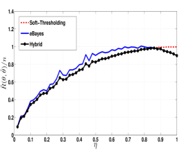
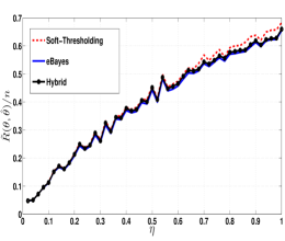
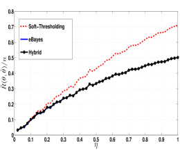
The performance of the hybrid estimator for the two kinds of $\boldsymbol{\theta}$ considered in Fig. 1 is highlighted in Fig. 2. Clearly, $n=1000$ is large enough for the hybrid estimator to accurately pick the better of $\hat{\boldsymbol{\theta}}_{ST}$ and $\hat{\boldsymbol{\theta}}_{EB}$. In both Figs. 1 and 2, $\epsilon$ was chosen equal to the true sparsity level $\eta$ for both estimators.

When the true sparsity level $\eta$ is unknown, one can optimize SURE to find the best choice of $\epsilon$ for both $\hat{\boldsymbol{\theta}}_{ST}$ and $\hat{\boldsymbol{\theta}}_{EB}$. The concentration results (Theorem 3 and Theorem 1) imply that the SURE for either estimator does not deviate much from the actual risk for large $n$. Donoho and Johnstone [3] have proposed SureShrink which chooses the thresholding parameter $\lambda^{*}$ from the interval $(0,\sqrt{2\log n}]$ as follows. The interval $(0,\sqrt{2\log n}]$ is discretized to define a discrete set $\mathcal{S}$. Then

$$\lambda^{*}=\operatorname*{arg\,min}_{\lambda\in\mathcal{S}}{\hat{R}(\boldsymbol{\theta},\hat{\boldsymbol{\theta}}_{ST}(\mathbf{y});\lambda)}/n$$ (5.1)

where $\hat{R}(\boldsymbol{\theta},\hat{\boldsymbol{\theta}}_{ST}(\mathbf{y});\lambda)$ is as defined in (3.1).

(a)

(b)

(c)

(d)

Figure 3: Average normalized loss $\tilde{R}(\boldsymbol{\theta},\hat{\boldsymbol{\theta}})/n$ with $n=1000$ for the following cases: a) The non-zero entries of $\boldsymbol{\theta}$ are drawn from $\mathcal{N}(0,1)$. b) The non-zero entries are drawn from the Laplace distribution with mean $0$ and variance $2$. c) The non-zero entries are drawn from the Rademacher (equiprobable $\pm 1$) distribution. d) The non-zero entries are drawn uniformly from $[-1,1]$.

(a)

(b)

(c)

(d)

Figure 4: Average normalized loss $\tilde{R}(\boldsymbol{\theta},\hat{\boldsymbol{\theta}})/n$ with the non-zero entries drawn from the Rademacher distribution for the following cases: a) $n=50$ b) $n=100$ c) $n=200$ d) $n=500$.

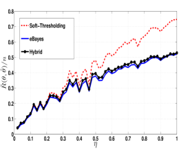
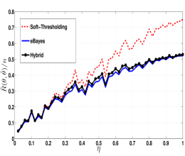
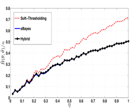
For the eBayes estimator, we propose to find the best value of $\epsilon$ in (2.4) by first discretizing the interval $(0,1]$ to define a discrete set $\mathcal{D}$, and choosing the sparsity parameter as

$$\epsilon^{*}=\operatorname*{arg\,min}_{\epsilon\in\mathcal{D}}{\hat{R}(\boldsymbol{\theta},\hat{\boldsymbol{\theta}}_{EB}(\mathbf{y});\epsilon)}/n.$$ (5.2)

Here $\hat{R}(\boldsymbol{\theta},\hat{\boldsymbol{\theta}}_{EB}(\mathbf{y});\epsilon)/n$ is as in (3.3), with suitable modifications to account for non-zero $\hat{\mu}$. The hybrid estimator then chooses the estimator with the lower value of SURE, i.e., by comparing $\hat{R}(\boldsymbol{\theta},\hat{\boldsymbol{\theta}}_{ST}(\mathbf{y});\lambda^{*})$ versus $\hat{R}(\boldsymbol{\theta},\hat{\boldsymbol{\theta}}_{EB}(\mathbf{y});\epsilon^{*})$.

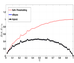
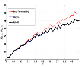
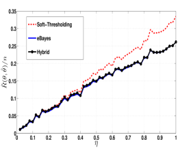
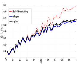
Fig. 3 shows the performance of the hybrid estimator at different sparsity levels for four choices for the distribution of the non-zero entries of $\boldsymbol{\theta}$: Gaussian (Fig. 3a), Laplacian (Fig. 3b), Rademacher (equiprobable $\pm 1$) (Fig. 3c), and uniform (Fig. 3d). We assume that the actual sparsity factor $\eta$ is unknown and use SURE to find the best sparsity parameters $\lambda^{*}$ and $\epsilon^{*}$ for $\hat{\boldsymbol{\theta}}_{ST}$ and $\hat{\boldsymbol{\theta}}_{EB}$, respectively. The optimization is performed over the discrete sets $\mathcal{S}=\{0.1i,i\in[\lceil 10\sqrt{2\log n}\rceil]\}$ and $\mathcal{D}=\{0.02i,i\in[50]\}$. In all the plots, $n=1000$. The plots suggest that for a wide range of $\boldsymbol{\theta}$, $\hat{\boldsymbol{\theta}}_{EB}$ is at least as good as $\hat{\boldsymbol{\theta}}_{ST}$ for all values of the sparsity factor $\eta$, and better in most cases.

Fig. 4 illustrates the performance of the hybrid estimator as a function of $n$. It shows the average normalized losses of the three estimators for different values of $n$ when the non-zero entries of $\boldsymbol{\theta}$ take values from the Rademacher distribution. These plots indicate that the proposed hybrid estimator performs very well even for relatively small values of $n$.

5.1 Application to Compressed Sensing

Given a measurement matrix $\mathbf{A}\in\mathbb{R}^{m\times n}$, the goal in compressed sensing [11, 12, 13] is to estimate a sparse vector $\boldsymbol{\theta}\in\mathbb{R}^{n}$ from a noisy linear measurement $\mathbf{y}\in\mathbb{R}^{m}$. In particular, consider the measurement model

$$\mathbf{y}=\mathbf{A}\boldsymbol{\theta}+\mathbf{w},$$

where $\mathbf{A}$ is an $m\times n$ random matrix with i.i.d. sub-Gaussian entries (normalized so that its columns have Euclidean norm concentrated around $1$), and the noise vector $\mathbf{w}\sim\mathcal{N}(\mathsf{0},\sigma^{2}\mathbf{I})$. The undersampling ratio is denoted by $\delta\vcentcolon=m/n<1$.

For this linear model, Approximate message passing (AMP) [14, 15, 24, 19, 17] is a class of low-complexity iterative algorithms to estimate $\boldsymbol{\theta}$ from $\mathbf{y}$. Starting with the initial conditions $\boldsymbol{\theta}_{0}=\mathsf{0}$, $\mathbf{z}_{0}=\mathbf{y}$, AMP iteratively produces estimates $\{\boldsymbol{\theta}_{t}\}$, for $t\geq 1$ as follows [15]:

$$\boldsymbol{\theta}_{t} =f_{t}\left(\mathbf{A}^{T}\mathbf{z}_{t-1}+\boldsymbol{\theta}_{t-1}\right)$$ (5.3)

$$\mathbf{z}_{t} =\mathbf{y}-\mathbf{A}\boldsymbol{\theta}_{t}+\frac{1}{\delta}\mathbf{z}_{t-1}\left\langle f_{t}^{\prime}\left(\mathbf{A}^{T}\mathbf{z}_{t-1}+\boldsymbol{\theta}_{t-1}\right)\right\rangle.$$ (5.4)

Here for each $t$, $f_{t}:\mathbb{R}\to\mathbb{R}$ is a “denoising” function, and $f^{\prime}_{t}$ denotes its derivative. For a vector input $\mathbf{u}\in\mathbb{R}^{n}$, both $f_{t}$ and $f^{\prime}_{t}$ operate component-wise on $\mathbf{u}$. Further, for $\mathbf{u}\in\mathbb{R}^{n}$, $\langle\mathbf{u}\rangle\vcentcolon=\frac{1}{n}\sum_{t=1}^{n}u_{t}$ denotes the average of its entries.

The AMP update (5.3) is underpinned by the following key property of the effective observation vector $(\mathbf{A}^{T}\mathbf{z}_{t}+\boldsymbol{\theta}^{t})$: for large $n$, after each iteration $t$, $(\mathbf{A}^{T}\mathbf{z}_{t}+\boldsymbol{\theta}^{t})$ is approximately distributed as $\boldsymbol{\theta}+\tau_{t}\mathbf{Z}$, where $\mathbf{Z}\in\mathbb{R}^{n}$ is an i.i.d. $\mathcal{N}(0,1)$ random vector independent of $\boldsymbol{\theta}$. The effective noise variance $\tau_{t}^{2}$ is determined (in the large system limit) by a scalar recursion called state evolution [15], [24]. For our purposes, it suffices to note that for each $t$, a good estimate of $\tau_{t}^{2}$ is given by $\widehat{\tau}_{t}^{2}\vcentcolon=\frac{\lVert\mathbf{z}_{t}\rVert^{2}}{m}$ (see, for example, [24, pp. 14,21], also [16, 35]).

Thus, the function $f_{t}$ estimates the sparse vector $\boldsymbol{\theta}$ from an observation in Gaussian noise of variance approximately $\widehat{\tau}_{t-1}^{2}=\frac{\lVert z^{t-1}\rVert^{2}}{m}$. Therefore, in each iteration, the AMP provides a platform to compare the performance of soft-thresholding and the eBayes estimator (and hence the hybrid estimator) as choices for $f_{t}$. We note that while soft-thresholding operates on a vector component-wise, the eBayes estimator doesn’t. However, for sufficiently large values of $m$ and $n$, both $\hat{\mu}$ and $\widehat{\xi^{2}}$ in (2.2)-(2.4) are close to deterministic values in which case the eBayes estimator also approximately acts component-wise on a vector. We remark that if we use soft-thresholding with the threshold in each iteration tuned to the noise-level $\tau_{t}$, the fixed points of the AMP algorithm coincide with that of the LASSO [24, 16].

(a)

(b)

(c)

(d)

Figure 5: Plots of the mean squared error $\lVert\boldsymbol{\theta}_{t}-\boldsymbol{\theta}\rVert^{2}/n$ as a function of the iteration number $t$ for the following cases, with $n=10,000$: a) $\delta=0.65$, $\eta=0.13$, $\sigma=1$, the non-zero entries of $\boldsymbol{\theta}$ are drawn from $\mathcal{N}(0,5)$. b) $\delta=0.65$, $\eta=0.13$, $\sigma=1$, the non-zero entries are drawn from the uniform distribution between $[-5,5]$. c) $\delta=0.5$, $\eta=0.1$, $\sigma=0$, the non-zero entries are drawn from the Rademacher distribution. d) $\delta=0.5$, $\eta=0.05$, $\sigma=0.05$, the non-zero entries are drawn from the Rademacher distribution. The state evolution (SE) prediction of the MSE for the hybrid estimator is also shown in the plots.

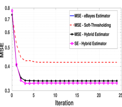
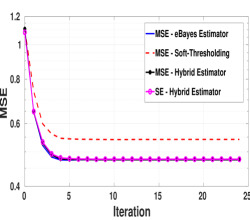
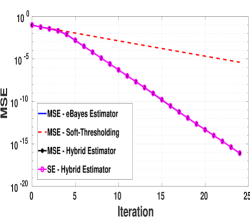
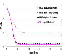
The simulation plots in Fig. 5 show the performances of the three estimators (soft-thresholding, the eBayes estimator, and the hybrid estimator) when used in the AMP algorithm. Throughout, we fix $n=10000$ but consider various values of the undersampling ratio $\delta=m/n$, the sparsity factor $\eta=\lVert\boldsymbol{\theta}\rVert_{0}/n$, the noise variance $\sigma^{2}$, and the non-zero values of $\boldsymbol{\theta}$. We choose such a large $n$ because the claim that $\mathbf{A}^{T}\mathbf{z}_{t}+\boldsymbol{\theta}^{t}\stackrel{{\scriptstyle\text{d}}}{{=}}\boldsymbol{\theta}+\tau_{t}\mathbf{Z}$ in every iteration $t$ holds in the large system limit. The measurement matrix $\mathbf{A}$ is chosen with its entries i.i.d. $\sim\mathcal{N}(0,1/m)$, and the sparsity factor $\eta$ is assumed to be unknown.

In each step of the algorithm, a suitable threshold $\lambda_{t}^{*}$ (for soft-thresholding), and a suitable sparsity parameter $\epsilon_{t}^{*}$ (for the eBayes estimator) are chosen as described in (5.1) and (5.2) with the only difference being that the risk estimates are now based on $\lVert\mathbf{z}_{t}\rVert^{2}/m$ and not on SURE. To be precise, the updates in iteration $t$ for each case are generated as follows:

1. Soft-thresholding: Let $\mathcal{S}\vcentcolon=\{0.1j,j\in[\lceil 10\sqrt{2\log n}\rceil]\}$. Then, for each $\lambda\in\mathcal{S}$, compute:

   $$\boldsymbol{\theta}_{t}(\lambda) =\hat{\boldsymbol{\theta}}_{ST}\left(\mathbf{A}^{T}\mathbf{z}_{t-1}+\boldsymbol{\theta}_{t-1};\lambda\widehat{\tau}_{t-1}\right),\ \ \text{ where }\widehat{\tau}_{t-1}=\lVert\mathbf{z}_{t-1}\rVert/\sqrt{m},$$

   $$\mathbf{z}_{t}(\lambda) =\mathbf{y}-\mathbf{A}\boldsymbol{\theta}_{t}(\lambda)+\frac{1}{\delta}\mathbf{z}_{t-1}\left\langle f_{t}^{\prime}\left(\mathbf{A}^{T}\mathbf{z}_{t-1}+\boldsymbol{\theta}_{t-1};\lambda\widehat{\tau}_{t-1}\right)\right\rangle.$$

   Then choose $\lambda_{t}^{*}=\operatorname*{arg\,min}_{\lambda\in\mathcal{S}}\,\lVert\mathbf{z}_{t}(\lambda)\rVert^{2}/m$, and generate the updated estimates

   $$\boldsymbol{\theta}_{t} =\boldsymbol{\theta}_{t}(\lambda_{t}^{*}),~{}~{}~{}~{}\mathbf{z}_{t}=\mathbf{z}_{t}(\lambda_{t}^{*}).$$

2. eBayes: Let $\mathcal{D}\vcentcolon=\{0.02j,j\in[50]\}$. Then, for each $\epsilon\in\mathcal{D}$, compute:

   $$\boldsymbol{\theta}_{t}(\epsilon) =\hat{\boldsymbol{\theta}}_{EB}\left(\mathbf{A}^{T}\mathbf{z}_{t-1}+\boldsymbol{\theta}_{t-1};\epsilon\right)\ \text{ where }\hat{\boldsymbol{\theta}}_{EB}\text{ is modified for noise level }\widehat{\tau}_{t-1}=\frac{\lVert\mathbf{z}_{t-1}\rVert}{\sqrt{m}},$$

   $$\mathbf{z}_{t}(\epsilon) =\mathbf{y}-\mathbf{A}\boldsymbol{\theta}_{t}(\epsilon)+\frac{1}{\delta}\mathbf{z}_{t-1}\left\langle f_{t}^{\prime}\left(\mathbf{A}^{T}\mathbf{z}_{t-1}+\boldsymbol{\theta}_{t-1};\epsilon\right)\right\rangle.$$

   Then choose $\epsilon_{t}^{*}=\operatorname*{arg\,min}_{\epsilon\in\mathcal{D}}\ \lVert\mathbf{z}_{t}(\epsilon)\rVert^{2}/m$, and generate the updated estimates

   $$\boldsymbol{\theta}_{t} =\boldsymbol{\theta}_{t}(\epsilon_{t}^{*}),~{}~{}~{}~{}\mathbf{z}_{t}=\mathbf{z}_{t}(\epsilon_{t}^{*}).$$

3. Hybrid estimator: In iteration $t$, $\boldsymbol{\theta}_{t}$ is set to either $\boldsymbol{\theta}_{t}(\lambda_{t}^{*})$ or $\boldsymbol{\theta}_{t}(\epsilon_{t}^{*})$ depending on which of $\lVert\mathbf{z}_{t}(\lambda_{t}^{*})\rVert^{2}$ and $\lVert\mathbf{z}_{t}(\epsilon_{t}^{*})\rVert^{2}$ is smaller.

The plots in Fig. 5 show the progression of the mean squared error (MSE) $\lVert\boldsymbol{\theta}_{t}-\boldsymbol{\theta}\rVert^{2}/n$ with the AMP iteration number $t$ for the three estimators when applied in the AMP algorithm for compressed sensing. We have also plotted the state evolution (SE) prediction of the MSE for the hybrid estimator (labelled “SE - Hybrid Estimator” on the plots), which for iteration $t$ is estimated as

$$\textrm{MSE}_{SE}(t)=\delta\left(\widehat{\tau}^{2}_{t}-\sigma^{2}\right)_{+},~{}~{}~{}~{}\text{ where }\widehat{\tau}^{2}_{t}=\frac{\min\left(\lVert\mathbf{z}_{t}(\lambda_{t}^{*})\rVert^{2},\lVert\mathbf{z}_{t}(\epsilon_{t}^{*})\rVert^{2}\right)}{m}.$$

It can be inferred that the eBayes estimator provides a strong alternative to soft-thresholding in the AMP framework.

Remark 1.

It was observed in numerical experiments that the optimal values $\lambda_{t}^{*}$ and $\epsilon_{t}^{*}$ do not vary much with the iteration index $t$. So, to reduce the computational load, one can compute $\lambda_{t}^{*}$ and $\epsilon_{t}^{*}$ in the first iteration (or the first few) alone, and then retain them for the rest of the steps.

Remark 2.

As evident in Fig. 5, the distinction between the MSEs for soft-thresholding and the eBayes estimator becomes clearer after the first few iterations. It has been observed in the experiments that for large values of $n$, the hybrid estimator picks the better estimator (eBayes estimator in the cases under consideration) with very high probability after around ten iterations. So, to further reduce the computational load, after a certain number of iterations (e.g., ten), one can continue with the most recent choice for the hybrid estimator.

Note 2.

The idea of using SURE to tune the parameters of the AMP denoising function $f_{t}$ has been previously used in [36, 37, 38]. In [36, 37], the authors tune the parameter of the soft-thresholding denoiser by using a gradient descent based algorithm to optimize an objective function defined via SURE. It is shown that the parameter estimates produced by this method converge to the asymptotically optimal values as the dimension grows. The paper [38] uses SURE to tune the parameters of AMP denoising functions chosen from certain parametric kernel families, but does not provide theoretical guarantees on the performance of the proposed approach.

Beyond the context of AMP, SURE has been used to design denoising functions for images in [39, 40]. In particular, [39] proposes a hybrid estimator which is a mixture of derivatives of Gaussians while [40] proposes an estimator that is a mixture of more general exponential functions.

6 Proofs

6.1 Mathematical Preliminaries

We list some lemmas that are used in the proofs of the theorems.

Lemma 6.1.

(a) (Hoeffding’s lemma) [34, Lemma 2.2]: Let $X$ be a random variable such that $\mathbb{E}X=0$ and $a\leq X\leq b$ almost surely. Then, for all $s\in\mathbb{R}$, $\mathbb{E}\left[e^{sX}\right]\leq\exp\left({\frac{s^{2}(b-a)^{2}}{8}}\right)$. Hence, $X$ is sub-Gaussian with variance factor $(b-a)^{2}/4$, and for any $t>0$,

$$\mathbb{P}\left(|X|\geq t\right)\leq 2e^{-\frac{2t^{2}}{(b-a)^{2}}}.$$

(b) (Hoeffding’s inequality) [34, Theorem 2.8] Let $X_{1},\ldots,X_{n}$ be independent random variables such that $X_{i}\in[a_{i},b_{i}]$ almost surely for $i\in[n]$. Then for any $t>0$,

$$\mathbb{P}\left(\left|\sum_{i=1}^{n}X_{i}-\mathbb{E}X_{i}\right|\geq t\right)\leq 2e^{-\frac{2t^{2}}{\sum_{i}(b_{i}-a_{i})^{2}}}.$$

Lemma 6.2.

[41, Thm. 8,9] Suppose $X_{i}$ are independent random variables satisfying $X_{i}\geq 0$, $\mathbb{E}[X_{i}^{2}]<\infty$, $\forall i\in[n]$. Let $X=\sum_{i=1}^{n}X_{i}$. Then, we have for any $t>0$,

$$\mathbb{P}(X-\mathbb{E}[X]\leq-t)\leq e^{-\frac{t^{2}}{2\sum_{i=1}^{n}\mathbb{E}[X_{i}^{2}]}}.$$

On the other hand, if $X_{i}\leq 0$ with $\mathbb{E}[X_{i}^{2}]<\infty$, $\forall i\in[n]$, then, we have for any $t>0$,

$$\mathbb{P}(X-\mathbb{E}[X]\geq t)\leq e^{-\frac{t^{2}}{2\sum_{i=1}^{n}\mathbb{E}[X_{i}^{2}]}}.$$

Lemma 6.3.

(Gaussian concentration inequality) [34, Thm 5.6]: Let $\mathbf{x}\sim\mathcal{N}(\boldsymbol{0},\mathbf{I})$ and let $f:\mathbb{R}^{n}\to\mathbb{R}$ denote an $L$-Lipschitz function, i.e., $\forall\mathbf{x}_{1},\mathbf{x}_{2}\in\mathbb{R}^{n}$, $|f(\mathbf{x}_{1})-f(\mathbf{x}_{2})|\leq L\|\mathbf{x}_{1}-\mathbf{x}_{2}\|$. Then, for all $t>0$,

$$\mathbb{P}\left(|f(\mathbf{x})-\mathbb{E}f(\mathbf{x})|\geq t\right)\leq 2e^{-\frac{t^{2}}{2L^{2}}}.$$

Lemma 6.4.

Let $y_{i}=\theta_{i}+w_{i}$, $w_{i}\sim\mathcal{N}(0,1)$ and $\theta_{i}$ are deterministic constants, for $i=1,2,\cdots,n$. Let $f(\mathbf{y})\vcentcolon=\frac{1}{n}\sum_{i=1}^{n}\frac{y_{i}^{2}}{\left(1+ce^{-ay_{i}^{2}}\right)^{p}}$, where $a,c$ are positive constants and $p$ is a positive integer. Then for any $t>0$, we have

$$\mathbb{P}\left(f(\mathbf{y})-\mathbb{E}\left[f(\mathbf{y})\right]\leq-t\right) \leq e^{-\frac{nk_{1}t^{2}}{\sum_{i}\theta_{i}^{4}/n}},\qquad\mathbb{P}\left(f(\mathbf{y})-\mathbb{E}\left[f(\mathbf{y})\right]\geq t\right)\leq e^{-\frac{nk_{2}\min(t,t^{2})}{\max(1,\|\boldsymbol{\theta}\|^{2}/n)}},$$

where $k_{1}$ and $k_{2}$ are absolute positive constants.

Proof.

See Appendix A. ∎

Lemma 6.5.

Let $y_{i}=\theta_{i}+w_{i}$, $w_{i}\sim\mathcal{N}(0,1)$, $i=1,2,\cdots,n$, and let $f(\mathbf{y})\vcentcolon=\frac{1}{n}\sum_{i=1}^{n}\frac{1}{1+ce^{-ay_{i}^{2}}}$ for any positive constants $a$ and $c$. Then, we have for any $t>0$,

$$\mathbb{P}\left(|f(\mathbf{y})-\mathbb{E}\left[f(\mathbf{y})\right]|\geq t\right) \leq 2e^{-2n(1+c^{2})t^{2}/c^{2}}.$$ (6.1)

Proof.

This is a straightforward application of Hoeffding’s inequality (Lemma 6.1(b)) after noting that $\frac{1}{1+ce^{-ay_{i}^{2}}}\in[\frac{1}{1+c},1)$. ∎

Lemma 6.6.

Let $y_{i}=\theta_{i}+w_{i}$, $w_{i}\sim\mathcal{N}(0,1)$, $i=1,2,\cdots,n$, and let $f(\mathbf{y})\vcentcolon=\frac{1}{n}\sum_{i=1}^{n}\frac{y_{i}^{2}e^{-a_{1}y_{i}^{2}}}{\left(1+ce^{-a_{2}y_{i}^{2}}\right)^{2}}$ for any positive constants $c$, $a_{1}$ and $a_{2}$. Then, we have for any $t>0$,

$$\mathbb{P}\left(f(\mathbf{y})-\mathbb{E}\left[f(\mathbf{y})\right]\leq-t\right) \leq e^{-\frac{nk_{1}t^{2}}{\sum\theta_{i}^{4}/n}},$$ (6.2)

$$\mathbb{P}\left(f(\mathbf{y})-\mathbb{E}\left[f(\mathbf{y})\right]\geq t\right) \leq e^{-\frac{nk_{2}\min(t,t^{2})}{\sum_{i}\theta_{i}^{2}/n}},$$ (6.3)

where $k_{1}$ and $k_{2}$ are absolute positive constants.

Proof.

The proof is along the lines of that for Lemma 6.4. Let $Z_{i}\vcentcolon=\frac{y_{i}^{2}e^{-a_{1}y_{i}^{2}}}{n\left(1+ce^{-a_{2}y_{i}^{2}}\right)^{p}}$. Since $Z_{i}$’s are non-negative, the lower tail bound follows from Lemma 6.2. As in Lemma 6.4, the proof for the upper tail involves showing that $\lVert\nabla g(\mathbf{y})\rVert^{2}$ is bounded, where $g(\mathbf{y})=\sqrt{f(\mathbf{y})}$. ∎

Lemma 6.7.

Let $y_{i}=\theta_{i}+w_{i}$, where $w_{i}\sim\mathcal{N}(0,1)$ and $\theta_{i}$, $i=1,2,\cdots,n$, are deterministic. Let $f_{1}(\mathbf{y})\vcentcolon=\frac{1}{n}\sum_{i=1}^{n}\frac{\theta_{i}y_{i}\mathsf{1}_{\{\theta_{i}y_{i}\geq 0\}}}{1+ce^{-ay_{i}^{2}}}$ and $f_{2}(\mathbf{y})\vcentcolon=\frac{1}{n}\sum_{i=1}^{n}\frac{\theta_{i}y_{i}\mathsf{1}_{\{\theta_{i}y_{i}\leq 0\}}}{1+ce^{-ay_{i}^{2}}}$, where $a,c$ are positive constants. Then for any $t>0$, we have

$$\mathbb{P}\left(f_{1}(\mathbf{y})-\mathbb{E}\left[f_{1}(\mathbf{y})\right]\geq t\right) \leq e^{-\frac{nt^{2}}{2(1+c)^{2}\sum_{i}\theta_{i}^{2}/n}},$$ (6.4)

$$\mathbb{P}\left(f_{2}(\mathbf{y})-\mathbb{E}\left[f_{2}(\mathbf{y})\right]\leq-t\right) \leq e^{-\frac{nt^{2}}{2(1+c)^{2}\sum_{i}\theta_{i}^{2}/n}},$$ (6.5)

where $k$ is an absolute positive constant.

Proof.

We let $Z_{i}\vcentcolon=\frac{\theta_{i}y_{i}}{n\left(1+ce^{-ay_{i}^{2}}\right)}$ and $f(\mathbf{y})=\sum_{i=1}^{n}Z_{i}$. Now,

$$\lVert\nabla f(\mathbf{y})\rVert^{2} =\sum_{i=1}^{n}\left(\frac{\partial f(\mathbf{y})}{\partial y_{i}}\right)^{2}=\sum_{i=1}^{n}\frac{\theta_{i}^{2}}{n^{2}}\left[\frac{1}{1+ce^{-ay_{i}^{2}}}+\frac{acy_{i}^{2}e^{-ay_{i}^{2}}}{(1+ce^{-ay_{i}^{2}})^{2}}\right]^{2}$$

$$\leq\sum_{i=1}^{n}\frac{\theta_{i}^{2}}{n^{2}}\left[\frac{1}{1+ce^{-ay_{i}^{2}}}+\frac{c}{(1+ce^{-ay_{i}^{2}})^{2}}\right]^{2}\leq\frac{(1+c)^{2}\lVert\boldsymbol{\theta}\rVert^{2}}{n^{2}}.$$ (6.6)

Now, let $\mathcal{R}\vcentcolon=\{\mathbf{y}\in\mathbb{R}^{n}~{}|~{}\theta_{i}y_{i}\geq 0,\forall i\in[n]\}$. Let $h:\mathbb{R}\to\mathbb{R}$ be the function defined as

$$h(y_{i})=\left\{\begin{array}[]{cc}y_{i}&\textrm{if }\theta_{i}y_{i}\geq 0,\\ 0&\textrm{otherwise}.\\ \end{array}\right.$$

For any $\mathbf{y}\in\mathbb{R}^{n}$, let $h(\mathbf{y})\in\mathbb{R}^{n}$ be the vector obtained by applying $h(\cdot)$ component-wise on the elements of $\mathbf{y}$. Since $f_{1}(\mathbf{y})=f_{1}(h(\mathbf{y}))$, we have for any $\mathbf{y}_{1},\mathbf{y}_{2}\in\mathbb{R}^{n}$,

$$|f_{1}(\mathbf{y}_{1})-f_{1}(\mathbf{y}_{2})|=|f_{1}(h(\mathbf{y}_{1}))-f_{1}(h(\mathbf{y}_{2}))| \overset{(a)}{=}\langle\nabla f(\mathbf{c}),h(\mathbf{y}_{1})-h(\mathbf{y}_{2})\rangle$$

$$\overset{(b)}{\leq}\lVert\nabla f(\mathbf{c})\rVert\|h(\mathbf{y}_{1})-h(\mathbf{y}_{2})\|\leq\lVert\nabla f(\mathbf{c})\rVert\|\mathbf{y}_{1}-\mathbf{y}_{2}\|$$

$$\leq L_{n}\|\mathbf{y}_{1}-\mathbf{y}_{2}\|$$

where step $(a)$ is due to the mean value theorem with $\mathbf{c}=h(\mathbf{y}_{1})+c(h(\mathbf{y}_{2})-h(\mathbf{y}_{1}))$ for some $c\in[0,1]$, step $(b)$ is due to the Cauchy-Schwarz inequality, and $L_{n}\vcentcolon=\sup_{\mathbf{y}\in\mathcal{R}}\{\lVert\nabla f(\mathbf{y})\rVert\}\leq(1+c)\lVert\boldsymbol{\theta}\rVert/n$ from (6.6). Therefore, using Lemma 6.3, we get (6.4) (note that we do not require the lower tail inequality for $f_{1}(\mathbf{y})$ in this paper). Proceeding in the same manner, it is straightforward to obtain the proof of (6.5). ∎

Lemma 6.8.

Let $\{X_{n}(\boldsymbol{\theta}),\boldsymbol{\theta}\in\mathbb{R}^{n}\}_{n\geq 1}$ be a sequence of random variables such that for any $t>0$,

$$\mathbb{P}(|X_{n}(\boldsymbol{\theta})|\geq t)\leq Ke^{-nk\min(t,t^{2})},$$

where $K$ and $k$ are positive constants. Then

$$\mathbb{E}|X_{n}(\boldsymbol{\theta})|\leq\frac{c_{1}}{\sqrt{n}}\left(1+\frac{c_{2}}{\sqrt{n}}\right),$$

where $c_{1}=\frac{K}{2}\sqrt{\frac{\pi}{k}}$, $c_{2}=\frac{2}{\sqrt{k\pi}}$.

Proof.

We have

$$\mathbb{E}\left[|X_{n}|\right] =\int_{0}^{\infty}\mathbb{P}\left(|X_{n}|>t\right)dt{~{}\leq}\int_{0}^{1}Ke^{-nkt^{2}}dt+\int_{1}^{\infty}Ke^{-nkt}dt$$

$$<\int_{0}^{\infty}Ke^{-nkt^{2}}dt+\int_{0}^{\infty}Ke^{-nkt}dt$$

$$=\frac{K}{\sqrt{nk}}\int_{0}^{\infty}e^{-x^{2}}dx+\frac{K}{nk}\int_{0}^{\infty}e^{-x}dx=\frac{c_{1}}{\sqrt{n}}\left(1+\frac{c_{2}}{\sqrt{n}}\right).$$

∎

Lemma 6.9.

(Concentration for sum of pseudo-Lipschitz function of sub-Gaussians [35, Lemma A.11]). Let $f:\mathbb{R}\to\mathbb{R}$ be a pseudo-Lipschitz function [15] of order 2 with pseudo-Lipschitz constant $L$, i.e., for any $x,y\in\mathbb{R}$, $|f(x)-f(y)|\leq L(1+|x|+|y|)|x-y|$. Let $\mathbf{z}\in\mathbb{R}^{n}$ be a random vector with entries i.i.d. sub-Gaussian random variables with variance factor $\nu$. Then, for any $t>0$,

$$\mathbb{P}\left(\frac{1}{n}\left|\sum_{i=1}^{n}f(z_{i})-\mathbb{E}[f(z_{i})]\right|\geq t\right)\leq 2e^{-nk\min(t,t^{2})}$$

where $k$ is some absolute constant (inversely proportional to $L^{2}$).

6.2 Proof of Theorem 1

To complete the proof in Sec. 4.1, we need to prove Lemmas 4.1 and 4.2. We start with the latter.

Proof of Lemma 4.2:

We want to obtain a bound for $\mathbb{P}(\left|f_{n}\right|\geq t)$, where

$$f_{n}\vcentcolon=\frac{a^{2}_{\mathbf{y}}}{n}\sum_{i=1}^{n}\frac{y_{i}^{2}}{\left(1+c_{\mathbf{y}}e^{-ay_{i}^{2}/2}\right)^{2}}-\frac{a^{2}}{n}\sum_{i=1}^{n}\mathbb{E}\left[\frac{y_{i}^{2}}{\left(1+ce^{-ay_{i}^{2}/2}\right)^{2}}\right],$$ (6.7)

with the deterministic values $a,c$ defined in (4.5). For brevity, we define $b\vcentcolon=\frac{\lVert\boldsymbol{\theta}\rVert^{2}}{n}$. Also define the event

$$\mathcal{E}\vcentcolon=\left\{\mathbf{y}\left|b-u\leq\frac{\lVert\mathbf{y}\rVert^{2}}{n}-1\leq b+u\right.\right\},$$ (6.8)

where $u>0$ will be specified later. From (4.3), we have $\mathbb{P}\left(\mathcal{E}^{c}\right)\leq 2e^{-nk\min(u,u^{2})}$. Therefore,

$$\begin{split}\mathbb{P}\left(|f_{n}|\geq t\right)&=\mathbb{P}\left(|f_{n}|\geq t,\mathcal{E}\right)+\mathbb{P}\left(|f_{n}|\geq t,\mathcal{E}^{c}\right)\\ &\leq\mathbb{P}(\mathcal{E})\mathbb{P}\left(|f_{n}|\geq t|\mathcal{E}\right)+2e^{-nk\min(u,u^{2})}\\ &=\mathbb{P}(\mathcal{E})\mathbb{P}\left(f_{n}\geq t|\mathcal{E}\right)+\mathbb{P}(\mathcal{E})\mathbb{P}\left(f_{n}\leq-t|\mathcal{E}\right)+2e^{-nk\min(u,u^{2})}.\end{split}$$ (6.9)

Now, when event $\mathcal{E}$ occurs, from the definition of $a_{\mathbf{y}}$ in (3.2) we have

$$\left[1-\frac{\epsilon}{b-u+\epsilon}\right]_{+}\leq a_{\mathbf{y}}\leq 1-\frac{\epsilon}{b+u+\epsilon}.$$

We therefore have the following lower and upper bounds:

$$a_{\mathbf{y}} \geq a_{L}\vcentcolon\max\left\{\frac{b-u}{b+\epsilon},\ 0\right\},$$ (6.10)

$$a_{\mathbf{y}} \leq a_{U}\vcentcolon=\min\left\{\frac{b+u}{b+\epsilon},\ 1\right\}.$$ (6.11)

Similarly when $\mathcal{E}$ occurs, $\frac{1-\epsilon}{\epsilon^{3/2}}\sqrt{\epsilon+[b-u]_{+}}\leq c_{\mathbf{y}}\leq\frac{1-\epsilon}{\epsilon^{3/2}}\sqrt{b+u+\epsilon}$, and we have the bounds

$$c_{\mathbf{y}}\geq c_{L} \vcentcolon=c-\kappa_{1}\min(u,b),$$ (6.12)

$$c_{\mathbf{y}}\leq c_{U} \vcentcolon=c+\kappa_{1}u,$$ (6.13)

where $\kappa_{1}\vcentcolon=\frac{c}{b+\epsilon}=\frac{1-\epsilon}{\epsilon^{3/2}\sqrt{b+\epsilon}}$. Using these bounds in the definition of $f_{n}$ in (6.7), we have

$$\mathbb{P}\left(f_{n}\geq t|\mathcal{E}\right)$$

$$\leq\mathbb{P}\left(\left.\frac{a_{U}^{2}}{n}\sum_{i=1}^{n}\frac{y_{i}^{2}}{\left(1+c_{L}e^{-a_{U}y_{i}^{2}/2}\right)^{2}}-\frac{a^{2}}{n}\sum_{i=1}^{n}\mathbb{E}\left[\frac{y_{i}^{2}}{\left(1+ce^{-ay_{i}^{2}/2}\right)^{2}}\right]\geq t\right|\mathcal{E}\right)$$

$$=\mathbb{P}\left(\left.\frac{a_{U}^{2}}{n}\sum_{i=1}^{n}\frac{y_{i}^{2}}{\left(1+c_{L}e^{-a_{U}y_{i}^{2}/2}\right)^{2}}-\frac{a_{U}^{2}}{n}\sum_{i=1}^{n}\mathbb{E}\left[\frac{y_{i}^{2}}{\left(1+c_{L}e^{-a_{U}y_{i}^{2}/2}\right)^{2}}\right]+\Delta_{1n}\geq t\right|\mathcal{E}\right),$$ (6.14)

where

$$\Delta_{1n}\vcentcolon=\frac{a_{U}^{2}}{n}\sum_{i=1}^{n}\mathbb{E}\left[\frac{y_{i}^{2}}{\left(1+c_{L}e^{-a_{U}y_{i}^{2}/2}\right)^{2}}\right]-\frac{a^{2}}{n}\sum_{i=1}^{n}\mathbb{E}\left[\frac{y_{i}^{2}}{\left(1+ce^{-ay_{i}^{2}/2}\right)^{2}}\right].$$ (6.15)

Next,

$$\begin{split}&\mathbb{P}\left(\left.\frac{a_{U}^{2}}{n}\sum_{i=1}^{n}\frac{y_{i}^{2}}{\left(1+c_{L}e^{-a_{U}y_{i}^{2}/2}\right)^{2}}-\frac{a_{U}^{2}}{n}\sum_{i=1}^{n}\mathbb{E}\left[\frac{y_{i}^{2}}{(1+c_{L}e^{-a_{U}y_{i}^{2}/2})^{2}}\right]\geq t\right|\mathcal{E}\right)\\ &\leq\frac{1}{\mathbb{P}(\mathcal{E})}{\mathbb{P}\left(\frac{a_{U}^{2}}{n}\sum_{i=1}^{n}\left(\frac{y_{i}^{2}}{\left(1+c_{L}e^{-a_{U}y_{i}^{2}/2}\right)^{2}}-\mathbb{E}\left[\frac{y_{i}^{2}}{(1+c_{L}e^{-a_{U}y_{i}^{2}/2})^{2}}\right]\right)\geq t\right)}\leq\frac{e^{-nk\min(t,t^{2})}}{\mathbb{P}(\mathcal{E})},\end{split}$$ (6.16)

where the last inequality follows from Lemma 6.4 after noting that $c_{L}\leq c$ and hence upper bounded, and $k$ is some absolute positive constant due to the assumption that $\sum_{i=1}^{n}\theta_{i}^{4}/n<\Lambda$. Next, it is shown in Appendix B that $\Delta_{1n}\leq\kappa_{3}u$, where $\kappa_{3}\leq 2\frac{(b+1)}{b}(1+a+\kappa_{1}a^{2}b)$ is an absolute positive constant. Using this bound on $\Delta_{1n}$ and (6.16) in (6.14) we obtain

$$\begin{split}&\mathbb{P}\left(\left.\frac{a_{U}^{2}}{n}\sum_{i=1}^{n}\frac{y_{i}^{2}}{\left(1+c_{L}e^{-a_{U}y_{i}^{2}/2}\right)^{2}}-\frac{a_{U}^{2}}{n}\sum_{i=1}^{n}\mathbb{E}\left[\frac{y_{i}^{2}}{\left(1+c_{L}e^{-a_{U}y_{i}^{2}/2}\right)^{2}}\right]+\Delta_{1n}\geq t+\kappa_{3}u\right|\mathcal{E}\right)\\ &\leq\frac{e^{-nk\min(t,t^{2})}}{\mathbb{P}(\mathcal{E})}.\end{split}$$

Choosing $u=t$, we finally have, from (6.14),

$$\mathbb{P}(\mathcal{E})\mathbb{P}\left(f_{n}\geq t\right|\mathcal{E})\leq e^{-nk\min(t,t^{2})}$$ (6.17)

for a suitable absolute positive constant $k$.

The lower tail bound is established as follows in a similar manner.

$$\mathbb{P}\left(f_{n}\leq-t\right|\mathcal{E})$$ (6.18)

$$\leq\mathbb{P}\left(\left.\frac{a_{L}^{2}}{n}\sum_{i=1}^{n}\frac{y_{i}^{2}}{\left(1+c_{U}e^{-a_{L}y_{i}^{2}/2}\right)^{2}}-\frac{a_{L}^{2}}{n}\sum_{i=1}^{n}\mathbb{E}\left[\frac{y_{i}^{2}}{\left(1+c_{U}e^{-ay_{i}^{2}/2}\right)^{2}}\right]-\Delta_{2n}\leq-t\right|\mathcal{E}\right),$$

where

$$\Delta_{2n}\vcentcolon=\frac{a^{2}}{n}\sum_{i=1}^{n}\mathbb{E}\left[\frac{y_{i}^{2}}{\left(1+ce^{-ay_{i}^{2}/2}\right)^{2}}\right]-\frac{a_{L}^{2}}{n}\sum_{i=1}^{n}\mathbb{E}\left[\frac{y_{i}^{2}}{\left(1+c_{U}e^{-a_{L}y_{i}^{2}/2}\right)^{2}}\right].$$ (6.19)

Next, we have

$$\mathbb{P}\left(\left.\frac{a_{L}^{2}}{n}\sum_{i=1}^{n}\frac{y_{i}^{2}}{\left(1+c_{U}e^{-a_{L}y_{i}^{2}/2}\right)^{2}}-\frac{a_{L}^{2}}{n}\sum_{i=1}^{n}\mathbb{E}\left[\frac{y_{i}^{2}}{\left(1+c_{U}e^{-a_{L}y_{i}^{2}/2}\right)^{2}}\right]\leq-t\right|\mathcal{E}\right)$$

$$\leq\frac{1}{\mathbb{P}(\mathcal{E})}\mathbb{P}\left(\frac{a_{L}^{2}}{n}\sum_{i=1}^{n}\left(\frac{y_{i}^{2}}{(1+c_{U}e^{-a_{L}y_{i}^{2}/2})^{2}}-\mathbb{E}\left[\frac{y_{i}^{2}}{(1+c_{U}e^{-a_{L}y_{i}^{2}/2})^{2}}\right]\right)\leq-t\right)\leq\frac{e^{-nkt^{2}}}{\mathbb{P}(\mathcal{E})},$$ (6.20)

where the last inequality uses Lemma 6.4, and $k$ is an absolute positive constant due to the assumption that $\sum_{i=1}^{n}\theta_{i}^{4}/n<\Lambda$. Next it is shown in Appendix B that $\Delta_{2n}\leq\kappa_{3}u$, where $\kappa_{3}\leq 2\frac{(b+1)}{b}(1+a+\kappa_{1}a^{2}b)$ is an absolute positive constant. Using this bound on $\Delta_{2n}$ and (6.20) in (6.18) we obtain

$$\mathbb{P}\left(\left.\frac{a_{L}^{2}}{n}\sum_{i=1}^{n}\frac{y_{i}^{2}}{\left(1+c_{U}e^{-a_{L}y_{i}^{2}/2}\right)^{2}}-\frac{a_{L}^{2}}{n}\sum_{i=1}^{n}\mathbb{E}\left[\frac{y_{i}^{2}}{\left(1+c_{U}e^{-ay_{i}^{2}/2}\right)^{2}}\right]-\Delta_{2n}\leq-t-\kappa_{3}u\right|\mathcal{E}\right)$$

$$\leq e^{-nkt^{2}}/\mathbb{P}(\mathcal{E}).$$

Choosing $u=t$, we finally have, from (6.18),

$$\mathbb{P}(\mathcal{E})\mathbb{P}\left(f_{n}\leq-t\right|\mathcal{E})\leq e^{-nkt^{2}}$$ (6.21)

for some suitable absolute positive constant $k$. So, using (6.17) and (6.21) in (6.9), we arrive at

$$\mathbb{P}\left(|f_{n}|\geq t\right)\leq 4e^{-nk\min(t,t^{2})}.$$

The proofs of the concentration inequalities for $g_{n}$, $h_{n}$, and $w_{n}$ are along similar lines to the steps from (6.14)-(6.21). In particular, the concentration inequality for $g_{n}$ involves the application of Lemma 6.4 as done in (6.16) and (6.20), and that for $h_{n}$ involves the application of Lemma 6.5 to obtain inequalities of the form (6.16) and (6.20). The concentration inequality for $w_{n}$ involves the application of Lemma 6.6 and is also similar to the steps from (6.14)-(6.21) with two notable differences:

1. First, we establish that both $(a_{U}^{2}c_{U}-a^{2}c)\leq p_{1}u$ and $(a^{2}c-a_{L}^{2}c_{L})\leq p_{2}u$ for some positive constants $p_{1},p_{2}$. This can be done using (6.10)–(6.13). Indeed, for $u\geq b$, $a_{U}=1$, and so $a_{U}^{2}c_{U}-a^{2}c\leq(1-a^{2})c+\kappa_{1}u\leq\frac{(1-a^{2})cu}{b}+\kappa_{1}u=p_{1}u$ where $p_{1}\vcentcolon=\frac{(1-a^{2})c}{b}+\kappa_{1}$. For $0\leq u<b$, $a_{U}^{2}c_{U}-a^{2}c$ is convex in $u$ and hence, it is clear that for any $u>0$, $a_{U}^{2}c_{U}-a^{2}c\leq p_{1}u$. Next, it is clear from (6.12) and (6.13) that for $0\leq u<b$, $a^{2}c-a_{L}^{2}c_{L}$ is a concave function, and is bounded by $a^{2}c$ for $u\geq b$. Hence, $a^{2}c-a_{L}^{2}c_{L}\leq p_{2}u$ for $u>0$, where $p_{2}$ is the derivative of $a^{2}c-a_{L}^{2}c_{L}$ at $u=0$, i.e., $p_{2}=3(a+2)c/(b+\epsilon)$.

2. Next, we use the above bounds to show that

   $$\frac{1}{n}\sum_{i=1}^{n}\mathbb{E}\left[\frac{a_{U}^{2}c_{U}^{2}y_{i}^{2}e^{-a_{L}y_{i}^{2}/2}}{\left(1+c_{L}e^{-a_{U}y_{i}^{2}/2}\right)^{2}}-\frac{a^{2}c^{2}y_{i}^{2}e^{-ay_{i}^{2}/2}}{\left(1+ce^{-ay_{i}^{2}/2}\right)^{2}}\right]\leq q_{1}u$$

   $$\frac{1}{n}\sum_{i=1}^{n}\mathbb{E}\left[\frac{a^{2}c^{2}y_{i}^{2}e^{-ay_{i}^{2}/2}}{\left(1+ce^{-ay_{i}^{2}/2}\right)^{2}}-\frac{a_{L}^{2}c_{L}^{2}y_{i}^{2}e^{-a_{U}y_{i}^{2}/2}}{\left(1+c_{U}e^{-a_{L}y_{i}^{2}/2}\right)^{2}}\right]\leq q_{2}u$$

   for some positive constants $q_{1}$ and $q_{2}$. This is done using steps similar to those used to bound $\Delta_{1n},\Delta_{2n}$ in Appendix B.

Proof of Lemma 4.1:

We show that $u_{n},v_{n},x_{n}$ are each bounded by order $1/n$ quantities, and then apply Lemma 6.1(a) to obtain the concentration result.

Concentration for $u_{n}$: As $b_{i}(\mathbf{y})\geq 1$ for all $i$, we have

$$\frac{1}{n}\sum_{i=1}^{n}\frac{y_{i}^{2}}{d_{\mathbf{y}}^{2}b_{i}(\mathbf{y})}\mathsf{1}_{\{\lVert\mathbf{y}\rVert^{2}>n\}} \leq\frac{1}{n}\sum_{i=1}^{n}\frac{y_{i}^{2}}{d_{\mathbf{y}}^{2}}\mathsf{1}_{\{\lVert\mathbf{y}\rVert^{2}>n\}}=\frac{\epsilon^{2}\left(\lVert\mathbf{y}\rVert^{2}/n\right)}{\left[\left(\lVert\mathbf{y}\rVert^{2}/n\right)-1+\epsilon\right]^{2}}\mathsf{1}_{\{\lVert\mathbf{y}\rVert^{2}>n\}}\leq 1.$$

Therefore,

$$\frac{4}{\epsilon n^{2}}\sum_{i=1}^{n}\frac{y_{i}^{2}}{d_{\mathbf{y}}^{2}b_{i}(\mathbf{y})}\mathsf{1}_{\{\lVert\mathbf{y}\rVert^{2}>n\}}\in\left[0,4/(n\epsilon)\right].$$

Applying Lemma 6.1(a), we obtain that for any $t>0$, $\mathbb{P}\left(|u_{n}|\geq t\right)\leq 2e^{-n^{2}kt^{2}}$ for a suitable positive constant $k$.

Concentration for $v_{n}$: As $d_{\mathbf{y}},b_{i}(\mathbf{y})\geq 1$, $1\leq i\leq n$, we have

$$\frac{1}{n}\sum_{i=1}^{n}\frac{a_{\mathbf{y}}y_{i}^{4}e^{-\frac{a_{\mathbf{y}}y_{i}^{2}}{2}}}{d_{\mathbf{y}}^{3/2}b_{i}^{2}(\mathbf{y})}\leq\frac{1}{n}\sum_{i=1}^{n}a_{\mathbf{y}}y_{i}^{4}e^{-\frac{a_{\mathbf{y}}y_{i}^{2}}{2}}.$$

Next, we show that

$$f(\mathbf{y}):=\frac{1}{n}\sum_{i=1}^{n}{a_{\mathbf{y}}y_{i}^{4}e^{-\frac{a_{\mathbf{y}}y_{i}^{2}}{2}}}\leq K,$$ (6.22)

where $K$ is a constant to be determined. Let $C>0$ be a constant to be fixed later. There are two cases:

1. $\lVert\mathbf{y}\rVert^{2}/n\leq 1+C$: In this case, use the bound $e^{-x}<\frac{1}{x}$ for all $x>0$. Using this we have

   $$f(\mathbf{y}):=\frac{1}{n}\sum_{i=1}^{n}{a_{\mathbf{y}}y_{i}^{4}e^{-\frac{a_{\mathbf{y}}y_{i}^{2}}{2}}}\,\leq\,\mathsf{1}_{\{\lVert\mathbf{y}\rVert^{2}>n\}}\frac{2}{n}\sum_{i=1}^{n}y_{i}^{2}\,\leq\,2(1+C)$$

   by assumption.

2. $\lVert\mathbf{y}\rVert^{2}/n>1+C$: In this case, from the definition of $a_{\mathbf{y}}$ in (3.2) note that $a_{\mathbf{y}}>C/(C+\epsilon)$. Now use the bound $e^{-x}<\frac{1}{x^{2}}$ for all $x>0$ to obtain

   $$f(\mathbf{y}):=\frac{1}{n}\sum_{i=1}^{n}{a_{\mathbf{y}}y_{i}^{4}e^{-\frac{a_{\mathbf{y}}y_{i}^{2}}{2}}}\leq\frac{4}{n}\sum_{i=1}^{n}\frac{1}{a_{\mathbf{y}}}<\frac{4(C+\epsilon)}{C}.$$

Choosing $C=(1+\sqrt{1+8\epsilon})/2$ to make the two bounds equal yields $K=3+\sqrt{1+8\epsilon}$. Therefore,

$$\frac{2(1-\epsilon)}{\epsilon^{2}n^{2}}\sum_{i=1}^{n}\frac{a_{\mathbf{y}}y_{i}^{4}e^{-\frac{a_{\mathbf{y}}y_{i}^{2}}{2}}}{d_{\mathbf{y}}^{3/2}b_{i}^{2}(\mathbf{y})}\in\left[0,\frac{2(1-\epsilon)K}{n\epsilon^{2}}\right].$$

Applying Lemma 6.1(a) yields, for any $t>0$,

$$\mathbb{P}\left(|v_{n}|\geq t\right)\leq 2e^{-n^{2}kt^{2}}$$

for a suitable positive constant $k$.

Concentration for $x_{n}$: Since $xe^{-x}\leq 1/e$ for $x>0$,

$$\frac{2(1-\epsilon)}{n^{2}\epsilon^{2}}\sum_{i=1}^{n}\frac{a_{\mathbf{y}}y_{i}^{2}e^{-\frac{a_{\mathbf{y}}y_{i}^{2}}{2}}}{\sqrt{d_{\mathbf{y}}}b_{i}^{2}(\mathbf{y})}\leq\frac{4(1-\epsilon)}{n\epsilon^{2}e}.$$

A direct application of Lemma 6.1(a) results in $\mathbb{P}\left(|x_{n}|\geq t\right)\leq 2e^{-n^{2}kt^{2}}$ for any $t>0$ and some positive constant $k$.

6.3 Proof of (4.14) for Theorem 2

The goal is to obtain a bound for $\mathbb{P}(\left|s_{n}\right|\geq t)$, where

$$s_{n}\vcentcolon=\frac{a_{\mathbf{y}}}{n}\sum_{i=1}^{n}\frac{\theta_{i}y_{i}}{1+c_{\mathbf{y}}e^{-ay_{i}^{2}/2}}-\frac{a}{n}\sum_{i=1}^{n}\mathbb{E}\left[\frac{\theta_{i}y_{i}}{1+ce^{-ay_{i}^{2}/2}}\right],$$ (6.23)

with the deterministic values $a,c$ defined in (4.5). Since the summands of the random term in (6.23) can take both positive and negative values, we employ the following approach to obtain the concentration inequality.

Let $s_{n}=s_{n}^{+}+s_{n}^{-}$ where

$$s_{n}^{+} \vcentcolon=\frac{a_{\mathbf{y}}}{n}\sum_{i=1}^{n}\frac{\theta_{i}y_{i}\mathsf{1}_{\{\theta_{i}y_{i}\geq 0\}}}{1+c_{\mathbf{y}}e^{-ay_{i}^{2}/2}}-\frac{a}{n}\sum_{i=1}^{n}\mathbb{E}\left[\frac{\theta_{i}y_{i}\mathsf{1}_{\{\theta_{i}y_{i}\geq 0\}}}{1+ce^{-ay_{i}^{2}/2}}\right],$$

$$s_{n}^{-} \vcentcolon=\frac{a_{\mathbf{y}}}{n}\sum_{i=1}^{n}\frac{\theta_{i}y_{i}\mathsf{1}_{\{\theta_{i}y_{i}\leq 0\}}}{1+c_{\mathbf{y}}e^{-ay_{i}^{2}/2}}-\frac{a}{n}\sum_{i=1}^{n}\mathbb{E}\left[\frac{\theta_{i}y_{i}\mathsf{1}_{\{\theta_{i}y_{i}\leq 0\}}}{1+ce^{-ay_{i}^{2}/2}}\right].$$

Using (6.8) and proceeding along the lines of (6.9), we obtain

$$\mathbb{P}\left(|s_{n}|\geq t\right) =\mathbb{P}\left(|s_{n}|\geq t,\mathcal{E}\right)+\mathbb{P}\left(|s_{n}|\geq t,\mathcal{E}^{c}\right)$$

$$\leq\mathbb{P}(\mathcal{E})\mathbb{P}\left(|s_{n}|\geq t|\mathcal{E}\right)+\mathbb{P}\left(\mathcal{E}^{c}\right)$$

$$\leq\mathbb{P}(\mathcal{E})\mathbb{P}\left(|s_{n}^{+}|\geq t/2|\mathcal{E}\right)+\mathbb{P}(\mathcal{E})\mathbb{P}\left(|s_{n}^{-}|\geq t/2|\mathcal{E}\right)+2e^{-nk\min(u,u^{2})}$$ (6.24)

where $u>0$ will be specified later. Now, with $a_{U}$ and $c_{L}$ as respectively defined in (6.11) and (6.12), we have

$$\mathbb{P}\left(s_{n}^{+}\geq t/2|\mathcal{E}\right) \leq\mathbb{P}\left(\left.\frac{a_{U}}{n}\sum_{i=1}^{n}\frac{\theta_{i}y_{i}\mathsf{1}_{\{\theta_{i}y_{i}\geq 0\}}}{1+c_{L}e^{-a_{U}y_{i}^{2}/2}}-\frac{a}{n}\sum_{i=1}^{n}\mathbb{E}\left[\frac{\theta_{i}y_{i}\mathsf{1}_{\{\theta_{i}y_{i}\geq 0\}}}{1+ce^{-ay_{i}^{2}/2}}\right]\geq t/2\right|\mathcal{E}\right)$$

$$=\mathbb{P}\left(\left.\frac{a_{U}}{n}\sum_{i=1}^{n}\frac{\theta_{i}y_{i}\mathsf{1}_{\{\theta_{i}y_{i}\geq 0\}}}{1+c_{L}e^{-a_{U}y_{i}^{2}/2}}-\frac{a_{U}}{n}\sum_{i=1}^{n}\mathbb{E}\left[\frac{\theta_{i}y_{i}\mathsf{1}_{\{\theta_{i}y_{i}\geq 0\}}}{1+c_{L}e^{-a_{U}y_{i}^{2}/2}}\right]+\Delta_{3n}\geq t/2\right|\mathcal{E}\right),$$ (6.25)

where

$$\Delta_{3n}\vcentcolon=\frac{a_{U}}{n}\sum_{i=1}^{n}\mathbb{E}\left[\frac{\theta_{i}y_{i}\mathsf{1}_{\{\theta_{i}y_{i}\geq 0\}}}{1+c_{L}e^{-a_{U}y_{i}^{2}/2}}\right]-\frac{a}{n}\sum_{i=1}^{n}\mathbb{E}\left[\frac{\theta_{i}y_{i}\mathsf{1}_{\{\theta_{i}y_{i}\geq 0\}}}{1+ce^{-ay_{i}^{2}/2}}\right].$$ (6.26)

Next,

$$\begin{split}&\mathbb{P}\left(\left.\frac{a_{U}}{n}\sum_{i=1}^{n}\frac{\theta_{i}y_{i}\mathsf{1}_{\{\theta_{i}y_{i}\geq 0\}}}{1+c_{L}e^{-a_{U}y_{i}^{2}/2}}-\frac{a_{U}}{n}\sum_{i=1}^{n}\mathbb{E}\left[\frac{\theta_{i}y_{i}\mathsf{1}_{\{\theta_{i}y_{i}\geq 0\}}}{1+c_{L}e^{-a_{U}y_{i}^{2}/2}}\right]\geq t/2\right|\mathcal{E}\right)\\ &\leq\frac{1}{\mathbb{P}(\mathcal{E})}{\mathbb{P}\left(\frac{a_{U}}{n}\sum_{i=1}^{n}\left(\frac{\theta_{i}y_{i}\mathsf{1}_{\{\theta_{i}y_{i}\geq 0\}}}{1+c_{L}e^{-a_{U}y_{i}^{2}/2}}-\mathbb{E}\left[\frac{\theta_{i}y_{i}\mathsf{1}_{\{\theta_{i}y_{i}\geq 0\}}}{1+c_{L}e^{-a_{U}y_{i}^{2}/2}}\right]\right)\geq t/2\right)}\leq\frac{e^{-n\kappa t^{2}}}{\mathbb{P}(\mathcal{E})},\end{split}$$ (6.27)

where the last inequality follows from Lemma 6.7, and $\kappa=(8a_{U}^{2}(1+c_{L})^{2}\lVert\boldsymbol{\theta}\rVert^{2}/n)^{-1}$. We note that $\kappa$ is bounded from below by an absolute positive constant due to Assumption A and the fact that $a_{U}\leq 1,c_{L}\leq c$ and hence bounded. Next, it is shown in Appendix B that $\Delta_{3n}\leq\kappa_{4}u$, where $\kappa_{4}\leq\sqrt{\frac{b+1}{b}}\left(2+\kappa_{1}ab\right)$ is an absolute positive constant. Using this bound on $\Delta_{3n}$ and (6.27) in (6.25) we obtain

$$\begin{split}&\mathbb{P}\left(\left.\frac{1}{n}\sum_{i=1}^{n}\frac{a_{U}\theta_{i}y_{i}}{1+c_{L}e^{-a_{U}y_{i}^{2}/2}}-\frac{1}{n}\sum_{i=1}^{n}\mathbb{E}\left[\frac{a_{U}\theta_{i}y_{i}}{1+c_{L}e^{-a_{U}y_{i}^{2}/2}}\right]+\Delta_{3n}\geq t/2+\kappa_{4}u\right|\mathcal{E}\right)\\ &\leq\frac{e^{-n\kappa t^{2}}}{\mathbb{P}(\mathcal{E})}.\end{split}$$

Choosing $u=t$, we finally have, from (6.25),

$$\mathbb{P}(\mathcal{E})\mathbb{P}\left(s_{n}^{+}\geq t/2\right|\mathcal{E})\leq e^{-nkt^{2}}$$ (6.28)

for a suitable absolute positive constant $k$.

To establish the lower tail, we proceed as follows. With $a_{L}$ and $c_{U}$ as respectively defined in (6.10) and (6.13), we have

$$\mathbb{P}\left(s_{n}^{+}\leq-t/2|\mathcal{E}\right) \leq\mathbb{P}\left(\left.\frac{a_{L}}{n}\sum_{i=1}^{n}\frac{\theta_{i}y_{i}\mathsf{1}_{\{\theta_{i}y_{i}\geq 0\}}}{1+c_{U}e^{-a_{L}y_{i}^{2}/2}}-\frac{a}{n}\sum_{i=1}^{n}\mathbb{E}\left[\frac{\theta_{i}y_{i}\mathsf{1}_{\{\theta_{i}y_{i}\geq 0\}}}{1+ce^{-ay_{i}^{2}/2}}\right]\leq-t/2\right|\mathcal{E}\right)$$

$$=\mathbb{P}\left(\left.\frac{a_{L}}{n}\sum_{i=1}^{n}\frac{\theta_{i}y_{i}\mathsf{1}_{\{\theta_{i}y_{i}\geq 0\}}}{1+c_{U}e^{-a_{L}y_{i}^{2}/2}}-\frac{a_{L}}{n}\sum_{i=1}^{n}\mathbb{E}\left[\frac{\theta_{i}y_{i}\mathsf{1}_{\{\theta_{i}y_{i}\geq 0\}}}{1+c_{U}e^{-a_{L}y_{i}^{2}/2}}\right]-\Delta_{4n}\leq-t/2\right|\mathcal{E}\right),$$ (6.29)

where

$$\Delta_{4n}\vcentcolon=\frac{a}{n}\sum_{i=1}^{n}\mathbb{E}\left[\frac{\theta_{i}y_{i}\mathsf{1}_{\{\theta_{i}y_{i}\geq 0\}}}{1+ce^{-ay_{i}^{2}/2}}\right]-\frac{a_{L}}{n}\sum_{i=1}^{n}\mathbb{E}\left[\frac{\theta_{i}y_{i}\mathsf{1}_{\{\theta_{i}y_{i}\geq 0\}}}{1+c_{U}e^{-a_{L}y_{i}^{2}/2}}\right].$$ (6.30)

Next,

$$\begin{split}&\mathbb{P}\left(\left.\frac{a_{L}}{n}\sum_{i=1}^{n}\frac{\theta_{i}y_{i}\mathsf{1}_{\{\theta_{i}y_{i}\geq 0\}}}{1+c_{U}e^{-a_{L}y_{i}^{2}/2}}-\frac{a_{L}}{n}\sum_{i=1}^{n}\mathbb{E}\left[\frac{\theta_{i}y_{i}\mathsf{1}_{\{\theta_{i}y_{i}\geq 0\}}}{1+c_{U}e^{-a_{L}y_{i}^{2}/2}}\right]\leq-t/2\right|\mathcal{E}\right)\\ &\leq\frac{1}{\mathbb{P}(\mathcal{E})}{\mathbb{P}\left(\frac{a_{L}}{n}\sum_{i=1}^{n}\left(\frac{\theta_{i}y_{i}\mathsf{1}_{\{\theta_{i}y_{i}\geq 0\}}}{1+c_{U}e^{-a_{L}y_{i}^{2}/2}}-\mathbb{E}\left[\frac{\theta_{i}y_{i}\mathsf{1}_{\{\theta_{i}y_{i}\geq 0\}}}{1+c_{U}e^{-a_{L}y_{i}^{2}/2}}\right]\right)\leq-t/2\right)}\leq\frac{e^{-nkt^{2}}}{\mathbb{P}(\mathcal{E})},\end{split}$$ (6.31)

where the last inequality follows from Lemma 6.2, and $k$ is some absolute positive constant due to Assumption A. Note that to obtain an inequality of the form (6.31), instead of Lemma 6.2, we cannot use a lower tail inequality result that is the counterpart of (6.4) because the constant $k$ would be proportional to $c_{U}^{-1}=(c+\kappa_{1}u)^{-1}$ which cannot be bounded from below unlike $c_{L}^{-1}$.

Next, it is shown in Appendix B that $\Delta_{4n}\leq\kappa_{4}u$. Using this bound on $\Delta_{4n}$ and (6.31) in (6.29) we obtain

$$\begin{split}&\mathbb{P}\left(\left.\frac{1}{n}\sum_{i=1}^{n}\frac{a_{L}\theta_{i}y_{i}}{1+c_{U}e^{-a_{L}y_{i}^{2}/2}}-\frac{1}{n}\sum_{i=1}^{n}\mathbb{E}\left[\frac{a_{L}\theta_{i}y_{i}}{1+c_{U}e^{-a_{L}y_{i}^{2}/2}}\right]-\Delta_{4n}\leq-t/2-\kappa_{4}u\right|\mathcal{E}\right)\leq\frac{e^{-nkt^{2}}}{\mathbb{P}(\mathcal{E})}.\end{split}$$

Choosing $u=t$, we finally have, from (6.29),

$$\mathbb{P}(\mathcal{E})\mathbb{P}\left(s_{n}^{+}\leq-t/2\right|\mathcal{E})\leq e^{-nkt^{2}}$$ (6.32)

for a suitable absolute positive constant $k$.

Hence, using (6.28) and (6.32), we arrive at

$$\mathbb{P}(\mathcal{E})\mathbb{P}\left(|s_{n}^{+}|\geq t|\mathcal{E}\right)\leq 2e^{-nkt^{2}}.$$ (6.33)

In a similar manner, it is straightforward to obtain

$$\mathbb{P}(\mathcal{E})\mathbb{P}\left(|s_{n}^{-}|\geq t|\mathcal{E}\right)\leq 2e^{-nkt^{2}}.$$ (6.34)

Using (6.33) and (6.34) in (6.24) and recalling that $u=t$, we finally obtain

$$\mathbb{P}\left(|s_{n}|\geq t\right)\leq 6e^{-nk\min(t,t^{2})}$$

for some suitable absolute positive constant $k$.

6.4 Proof of Theorem 4

For $i\in[n]$, let

$$h(w_{i})\vcentcolon=\hat{\theta}_{ST,i}-\theta_{i}=\left\{\begin{array}[]{cc}-\theta_{i},&-\lambda-\theta_{i}<w_{i}<\lambda-\theta_{i}\\ w_{i}-\lambda,&w_{i}\geq\lambda-\theta_{i}\\ w_{i}+\lambda,&w_{i}\leq-\lambda-\theta_{i}\\ \end{array}\right.$$

where $w_{i}\sim\mathcal{N}(0,1)$. Let $g(w_{i})\vcentcolon=(\hat{\theta}_{ST,i}-\theta_{i})^{2}$. We show that $g$ is pseudo-Lipschitz of order $2$ with pseudo-Lipschitz constant $\max(1,2\lambda)$, and then apply Lemma 6.9 to arrive at (4.18). It is straightforward to note that $h$ is Lipschitz with Lipschitz constant $1$, i.e., $|h(x)-h(y)|\leq|x-y|$, $\forall x,y\in\mathbb{R}$. Now, for any $w_{i,1},w_{i,2}\in\mathbb{R}$,

$$|g(w_{i,1})-g(w_{i,2})| =|h(w_{i,1})+h(w_{i,2})||h(w_{i,1})-h(w_{i,2})|$$

$$\leq|h(w_{i,1})+h(w_{i,2})||w_{i,1}-w_{i,2}|$$

$$\leq(|h(w_{i,1})|+|h(w_{i,2})|)|w_{i,1}-w_{i,2}|$$

$$\leq\left(2\lambda+|w_{i,1}|+|w_{i,2}|\right)|w_{i,1}-w_{i,2}|$$

$$\leq\max(1,2\lambda)\left(1+|w_{i,1}|+|w_{i,2}|\right)|w_{i,1}-w_{i,2}|.$$

Hence, we obtain the pseudo-Lipschitz constant $L$ to be $\max(1,2\lambda)$. Therefore, we can apply Lemma 6.9 to obtain the desired concentration result (4.18) for $\frac{1}{n}\sum_{i=1}^{n}g(w_{i})=\frac{1}{n}\sum_{i=1}^{n}(\hat{\theta}_{ST,i}-\theta_{i})^{2}$.

6.5 Proof of Theorem 5

Without loss of generality, for a chosen $t>0$, we can assume that

$$\frac{1}{n}L_{sep}(\boldsymbol{\theta},\mathbf{y})>t+\kappa_{n}$$ (6.35)

because otherwise, it is clear that

$$\frac{1}{n}L(\boldsymbol{\theta},\hat{\boldsymbol{\theta}}_{H}(\mathbf{y}))\leq\frac{1}{n}L_{min}(\boldsymbol{\theta},\mathbf{y})+t+\kappa_{n}$$

and (4.21) trivially holds. In what follows, we use $K$ and $k$ as generic universal constants that appear in the concentration inequalities. These constants are independent of $n$, but their values change as we proceed through the proof.

Let us first suppose that $\hat{\boldsymbol{\theta}}_{EB}$ is the better estimator of $\boldsymbol{\theta}$ for the given realization $\mathbf{y}$. Then, recalling the definition of $\gamma_{\mathbf{y}}$ in (3.7), the desired probability can be bounded as

$$\mathbb{P}\left(\frac{1}{n}L(\boldsymbol{\theta},\hat{\boldsymbol{\theta}}_{H}(\mathbf{y}))\geq\frac{1}{n}L(\boldsymbol{\theta},\hat{\boldsymbol{\theta}}_{EB}(\mathbf{y}))+t+\kappa_{n}\right)$$

$$\leq\mathbb{P}(\gamma_{\mathbf{y}}=0)=\mathbb{P}\left(\frac{1}{n}\hat{R}(\boldsymbol{\theta},\hat{\boldsymbol{\theta}}_{EB}(\mathbf{y}))-\frac{1}{n}\hat{R}(\boldsymbol{\theta},\hat{\boldsymbol{\theta}}_{ST}(\mathbf{y}))>0\right).$$ (6.36)

The RHS of (6.36) is bounded as follows. Using the triangle inequality, we have for any $u>0$,

$$\mathbb{P}\left(\left|\frac{1}{n}\hat{R}(\boldsymbol{\theta},\hat{\boldsymbol{\theta}}_{EB}(\mathbf{y}))-\frac{1}{n}L(\boldsymbol{\theta},\hat{\boldsymbol{\theta}}_{EB}(\mathbf{y}))\right|\geq u+\kappa_{n}\right)$$

$$\leq\mathbb{P}\left(\frac{1}{n}\left|L(\boldsymbol{\theta},\hat{\boldsymbol{\theta}}_{EB}(\mathbf{y}))-R_{2}(\boldsymbol{\theta},\hat{\boldsymbol{\theta}}_{EB})\right|+\frac{1}{n}\left|\hat{R}(\boldsymbol{\theta},\hat{\boldsymbol{\theta}}_{EB}(\mathbf{y}))-R_{1}(\boldsymbol{\theta},\hat{\boldsymbol{\theta}}_{EB})\right|\right.$$

$$\qquad\qquad\left.+\frac{1}{n}\left|R_{2}(\boldsymbol{\theta},\hat{\boldsymbol{\theta}}_{EB})-R_{1}(\boldsymbol{\theta},\hat{\boldsymbol{\theta}}_{EB})\right|\geq u+\kappa_{n}\right)$$

$$\stackrel{{\scriptstyle(a)}}{{\leq}}\mathbb{P}\left(\frac{1}{n}\left|L(\boldsymbol{\theta},\hat{\boldsymbol{\theta}}_{EB}(\mathbf{y}))-R_{2}(\boldsymbol{\theta},\hat{\boldsymbol{\theta}}_{EB})\right|\geq\frac{u}{2}\right)+\mathbb{P}\left(\frac{1}{n}\left|\hat{R}(\boldsymbol{\theta},\hat{\boldsymbol{\theta}}_{EB}(\mathbf{y}))-R_{1}(\boldsymbol{\theta},\hat{\boldsymbol{\theta}}_{EB})\right|\geq\frac{u}{2}\right)$$

$$\stackrel{{\scriptstyle(b)}}{{\leq}}Ke^{-nk\min(u,u^{2})},$$ (6.37)

where inequality $(a)$ uses the definition of $\kappa_{n}$ in (4.20), and inequality $(b)$ is obtained using (4.1) and (4.11). Similarly, using (4.17) and (4.18), we obtain for any $u>0$,

$$\mathbb{P}\left(\frac{1}{n}\left|L(\boldsymbol{\theta},\hat{\boldsymbol{\theta}}_{ST}(\mathbf{y}))-\hat{R}(\boldsymbol{\theta},\hat{\boldsymbol{\theta}}_{ST}(\mathbf{y}))\right|\geq u\right)\leq 4e^{-nk\min(u,u^{2})}.$$ (6.38)

Combining (6.37) and (6.38), and using the definition of $L_{sep}$ in (4.19), we have for $u>0$

$$\mathbb{P}\left(\frac{1}{n}\hat{R}(\boldsymbol{\theta},\hat{\boldsymbol{\theta}}_{EB}(\mathbf{y}))-\frac{1}{n}\hat{R}(\boldsymbol{\theta},\hat{\boldsymbol{\theta}}_{ST}(\mathbf{y}))+\frac{L_{sep}(\boldsymbol{\theta},\mathbf{y})}{n}>2u+\kappa_{n}\right) \leq Ke^{-nk\min(u,u^{2})}.$$ (6.39)

Now, choosing $2u=\frac{L_{sep}(\boldsymbol{\theta},\mathbf{y})}{n}-\kappa_{n}$ (which is at least $t$ by the assumption (6.35)) yields

$$\mathbb{P}\left(\frac{1}{n}\hat{R}(\boldsymbol{\theta},\hat{\boldsymbol{\theta}}_{EB}(\mathbf{y}))-\frac{1}{n}\hat{R}(\boldsymbol{\theta},\hat{\boldsymbol{\theta}}_{ST}(\mathbf{y}))>0\right)\leq Ke^{-nk\min(t,t^{2})}.$$

Using this in (6.36), and noting that the other case ($\hat{\boldsymbol{\theta}}_{ST}$ is the better estimator) can be similarly analysed, we arrive at the concentration result (4.21).

To prove (4.23), let $X_{n}\vcentcolon=\frac{1}{n}\left[L(\boldsymbol{\theta},\hat{\boldsymbol{\theta}}_{H}(\mathbf{y}))-L_{min}(\boldsymbol{\theta},\mathbf{y})\right]\geq 0$. We have,

$$\mathbb{E}\left[X_{n}\right] =\int_{0}^{\infty}\mathbb{P}\left(X_{n}\geq u\right)du=\int_{0}^{\kappa_{n}}\mathbb{P}\left(X_{n}\geq u\right)du+\int_{\kappa_{n}}^{\infty}\mathbb{P}\left(X_{n}\geq u\right)du$$

$$\leq\int_{0}^{\kappa_{n}}du+\int_{\kappa_{n}}^{\infty}\mathbb{P}\left(X_{n}\geq u\right)du=\kappa_{n}+\int_{0}^{\infty}\mathbb{P}\left(X_{n}\geq t+\kappa_{n}\right)dt.$$

Note that $\kappa_{n}$ is an $\mathcal{O}(1/\sqrt{n})$ term. So, using (4.21) and the steps of the proof of Lemma 6.8, we obtain

$$\mathbb{E}\left[X_{n}\right]\leq\kappa_{n}+\int_{0}^{\infty}Ke^{-nk\min(t,t^{2})}dt\leq\kappa_{n}+\frac{C}{\sqrt{n}}\left(1+\frac{1}{\sqrt{n}}\right)$$

for some positive constant $C$. So,

$$\frac{R(\boldsymbol{\theta},\hat{\boldsymbol{\theta}}_{H})}{n}\leq\frac{\mathbb{E}\left[L_{min}(\boldsymbol{\theta},\mathbf{y})\right]}{n}+\kappa_{n}+\frac{C}{\sqrt{n}}\left(1+\frac{1}{\sqrt{n}}\right).$$ (6.40)

It trivially follows that $\mathbb{E}\left[L_{min}(\boldsymbol{\theta},\mathbf{y})\right]\leq\min\{R(\boldsymbol{\theta},\hat{\boldsymbol{\theta}}_{EB}),R(\boldsymbol{\theta},\hat{\boldsymbol{\theta}}_{ST})\}$. Using this in (6.40) and noting that $\kappa_{n}=\mathcal{O}(1/\sqrt{n})$ completes the proof of (4.23).

Funding

This work was supported by the European Commission [Marie Curie Career Integration Grant, Agreement Number 631489]; the Isaac Newton Trust; and the Engineering and Physical Sciences Research Council [EP/N013999/1].

Appendix A Proof of Lemma 6.4

Let $Z_{i}\vcentcolon=\frac{y_{i}^{2}}{n\left(1+ce^{-ay_{i}^{2}}\right)^{p}}$. Since $Z_{i}\geq 0$, from Lemma 6.2, we have

$$\mathbb{P}\left(f(\mathbf{y})-\mathbb{E}\left[f(\mathbf{y})\right]\leq-t\right)\leq e^{-nt^{2}/\mathsf{k}}$$ (A.1)

where $\mathsf{k}={2n\sum_{i=1}^{n}\mathbb{E}[Z_{i}^{2}]}\leq{\frac{2}{n}\sum_{i=1}^{n}\mathbb{E}[y_{i}^{4}]}=\frac{2}{n}\sum_{i=1}^{n}\left(\theta_{i}^{4}+6\theta_{i}^{2}+6\right)$. To prove the upper tail inequality we proceed as follows. For $g:\mathbb{R}^{n}\to\mathbb{R}$ which is differentiable, we have [42, Sec. 2.3]

$$\mathbb{E}\left[e^{s\{g(\mathbf{y})-\mathbb{E}[g(\mathbf{y})]\}}\right]\leq\mathbb{E}\left[e^{{s^{2}\pi^{2}\lVert\nabla g(\mathbf{y})\rVert^{2}}/{8}}\right].$$ (A.2)

We take $g(\mathbf{y})\vcentcolon=\sqrt{f(\mathbf{y})}$, and obtain an upper tail bound for $g$ by showing that $\lVert\nabla g(\mathbf{y})\rVert^{2}$ is bounded. Now,

$$\frac{\partial g(\mathbf{y})}{\partial w_{i}}=\frac{y_{i}\left[1+ce^{-ay_{i}^{2}}+pacy_{i}^{2}e^{-ay_{i}^{2}}\right]}{\sqrt{n}\left(1+ce^{-ay_{i}^{2}}\right)^{{p}+1}\sqrt{\sum_{j=1}^{n}{y_{j}^{2}}/\left(1+ce^{-ay_{j}^{2}}\right)^{p}}}.$$

Hence,

$$n\lVert\nabla g(\mathbf{y})\rVert^{2} =\frac{1}{{\sum_{j=1}^{n}{y_{j}^{2}}/\left(1+ce^{-ay_{j}^{2}}\right)^{p}}}\sum_{i=1}^{n}\frac{y_{i}^{2}\left[1+ce^{-ay_{i}^{2}}+pc\,ay_{i}^{2}e^{-ay_{i}^{2}}\right]^{2}}{\left(1+ce^{-ay_{i}^{2}}\right)^{{2p}+2}}$$

$$=\frac{1}{{\sum_{j=1}^{n}{y_{j}^{2}}/\left(1+ce^{-ay_{j}^{2}}\right)^{p}}}\sum_{i=1}^{n}\frac{y_{i}^{2}}{\left(1+ce^{-ay_{i}^{2}}\right)^{p}}\frac{\left[1+ce^{-ay_{i}^{2}}+pc\,ay_{i}^{2}e^{-ay_{i}^{2}}\right]^{2}}{\left(1+ce^{-ay_{i}^{2}}\right)^{{p}+2}}$$

$$\leq\frac{1}{{\sum_{j=1}^{n}{y_{j}^{2}}/\left(1+ce^{-ay_{j}^{2}}\right)^{p}}}\sum_{i=1}^{n}\frac{y_{i}^{2}}{\left(1+ce^{-ay_{i}^{2}}\right)^{p}}\left[1+\frac{pc\,ay_{i}^{2}e^{-ay_{i}^{2}}}{\left(1+ce^{-ay_{i}^{2}}\right)^{{p/2}+1}}\right]^{2}.$$

Using the bound $ay_{i}^{2}e^{-ay_{i}^{2}}\leq 1/e$, we obtain

$$n\lVert\nabla g(\mathbf{y})\rVert^{2}\leq C$$

where $C\vcentcolon=\left(1+\frac{pc}{e}\right)^{2}$. Hence,

$$\mathbb{E}\left[e^{s\{g(\mathbf{y})-\mathbb{E}[g(\mathbf{y})]\}}\right]\leq e^{{s^{2}\pi^{2}C}/{8n}}.$$

Hence, $g(\mathbf{y})$ is sub-Gaussian [34, Sec. 2.3] with variance factor at most $\frac{\pi^{2}C}{4n}$. Therefore, using the Cramér-Chernoff bound, we have for $t>0$:

$$\mathbb{P}\left(g(\mathbf{y})\geq\mathbb{E}\left[g(\mathbf{y})\right]+t\right)\leq e^{-{2nt^{2}}/{\pi^{2}C}}.$$ (A.3)

Recalling that $g(\mathbf{y})=\sqrt{f(\mathbf{y})}$ and using Jensen’s inequality, we have $\mathbb{E}\left[f(\mathbf{y})\right]=\mathbb{E}\left[g^{2}(\mathbf{y})\right]\geq\left(\mathbb{E}\left[g(\mathbf{y})\right]\right)^{2}$. We therefore have

$$\mathbb{P}\left(f(\mathbf{y})\geq\mathbb{E}\left[f(\mathbf{y})\right]+t^{2}+2t\mathbb{E}\left[g(\mathbf{y})\right]\right) \leq\mathbb{P}\left(f(\mathbf{y})\geq\left(\mathbb{E}\left[g(\mathbf{y})\right]\right)^{2}+t^{2}+2\mathbb{E}\left[g(\mathbf{y})\right]t\right)$$

$$=\mathbb{P}\left(g(\mathbf{y})\geq\mathbb{E}\left[g(\mathbf{y})\right]+t\right)$$

$$\leq e^{-{2nt^{2}}/{\pi^{2}C}},$$ (A.4)

where the last inequality follows from (A.3). Note that

$$t^{2}+2t\mathbb{E}[g(\mathbf{y})]\leq\left\{\begin{array}[]{cc}t^{2}(1+2\mathbb{E}[g(\mathbf{y})])&\textrm{when }t\geq 1,\\ t(1+2\mathbb{E}[g(\mathbf{y})])&\textrm{otherwise},\\ \end{array}\right.$$

and recall that $(\mathbb{E}\left[g(\mathbf{y})\right])^{2}\leq\mathbb{E}f(\mathbf{y})\leq\|\boldsymbol{\theta}\|^{2}/n+1$. Now, setting $u=\max(t,t^{2})(1+2\sqrt{1+\|\boldsymbol{\theta}\|^{2}/n})$, from (A.4) we obtain,

$$\mathbb{P}\left(f(\mathbf{y})\geq\mathbb{E}\left[f(\mathbf{y})\right]+u\right)\leq\mathbb{P}\left(f(\mathbf{y})\geq\mathbb{E}\left[f(\mathbf{y})\right]+t^{2}+2t\mathbb{E}\left[g(\mathbf{y})\right]\right)\leq e^{-{2nt^{2}}/{\pi^{2}C}}.$$

Therefore, we have, for every $u>0$:

$$\mathbb{P}\left(f(\mathbf{y})-\mathbb{E}\left[f(\mathbf{y})\right]\geq u\right)\leq e^{-nk\min(u,u^{2})/\max(1,\|\boldsymbol{\theta}\|^{2}/n)}$$ (A.5)

for a suitable absolute positive constant $k$. Combining (A.1) and (A.5) completes the proof.

Appendix B Bounds on $\Delta_{1n},\Delta_{2n}$, $\Delta_{3n}$, $\Delta_{4n}$

Bound on $\Delta_{1n}$: Recall that $a=\frac{b}{b+\epsilon}$ and $a_{U}=\min\{\frac{b+u}{b+\epsilon},1\}$. Hence, $a_{U}-a\leq u/b$, and it follows that $a_{U}^{2}-a^{2}=(a_{U}-a)(a_{U}+a)\leq\frac{2}{b}u$. We therefore have

$$\Delta_{1n}=\frac{a_{U}^{2}}{n}\sum_{i=1}^{n}\mathbb{E}\left[\frac{y_{i}^{2}}{\left(1+c_{L}e^{-a_{U}y_{i}^{2}/2}\right)^{2}}\right]-\frac{a^{2}}{n}\sum_{i=1}^{n}\mathbb{E}\left[\frac{y_{i}^{2}}{\left(1+ce^{-ay_{i}^{2}/2}\right)^{2}}\right]$$

$$\leq\frac{(a^{2}+(2/b)u)}{n}\sum_{i=1}^{n}\mathbb{E}\left[\frac{y_{i}^{2}}{\left(1+c_{L}e^{-a_{U}y_{i}^{2}/2}\right)^{2}}\right]-\frac{a^{2}}{n}\sum_{i=1}^{n}\mathbb{E}\left[\frac{y_{i}^{2}}{\left(1+ce^{-ay_{i}^{2}/2}\right)^{2}}\right]$$

$$=\frac{a^{2}}{n}\sum_{i=1}^{n}\mathbb{E}\left[\frac{y_{i}^{2}}{\left(1+c_{L}e^{-a_{U}y_{i}^{2}/2}\right)^{2}}-\frac{y_{i}^{2}}{\left(1+ce^{-ay_{i}^{2}/2}\right)^{2}}\right]+\frac{(2/b)u}{n}\sum_{i=1}^{n}\mathbb{E}\left[\frac{y_{i}^{2}}{\left(1+c_{L}e^{-a_{U}y_{i}^{2}/2}\right)^{2}}\right]$$

$$\leq\frac{a^{2}}{n}\sum_{i=1}^{n}\mathbb{E}\left[y_{i}^{2}\left(\frac{\left(ce^{-ay_{i}^{2}/2}-c_{L}e^{-a_{U}y_{i}^{2}/2}\right)\left(2+c_{L}e^{-a_{U}y_{i}^{2}/2}+ce^{-ay_{i}^{2}/2}\right)}{\left(1+c_{L}e^{-a_{U}y_{i}^{2}/2}\right)^{2}\left(1+ce^{-ay_{i}^{2}/2}\right)^{2}}\right)\right]+\frac{2u}{b}\mathbb{E}\left[\frac{\lVert\mathbf{y}\rVert^{2}}{n}\right]$$

$$\leq\frac{a^{2}}{n}\sum_{i=1}^{n}\mathbb{E}\left[2y_{i}^{2}\left(\frac{ce^{-ay_{i}^{2}/2}\left(1-e^{-(a_{U}-a)y_{i}^{2}/2}\right)+\kappa_{1}ue^{-a_{U}y_{i}^{2}/2}}{\left(1+c_{L}e^{-a_{U}y_{i}^{2}/2}\right)\left(1+ce^{-ay_{i}^{2}/2}\right)}\right)\right]+\frac{2(b+1)u}{b},$$ (B.1)

where the last inequality holds because the definition of $c_{L}$ in (6.12) implies $c-c_{L}\leq\kappa_{1}u$ . Now, $ce^{-ay_{i}^{2}/2}\left(1-e^{-(a_{U}-a)y_{i}^{2}/2}\right)$ has a maximum when $e^{-(a_{U}-a)y_{i}^{2}/2}=a/a_{U}$, and so,

$$\frac{ce^{-ay_{i}^{2}/2}\left(1-e^{-(a_{U}-a)y_{i}^{2}/2}\right)+\kappa_{1}ue^{-a_{U}y_{i}^{2}/2}}{\left(1+c_{L}e^{-a_{U}y_{i}^{2}/2}\right)\left(1+ce^{-ay_{i}^{2}/2}\right)} \leq 1-\frac{a}{a_{U}}+\kappa_{1}u\leq\frac{1}{ab}u+\kappa_{1}u.$$ (B.2)

Using this in (B.1), we obtain

$$\Delta_{1n}\leq\kappa_{3}u,$$ (B.3)

where $\kappa_{3}=2\frac{(b+1)}{b}(1+a+\kappa_{1}a^{2}b)u$.

Bound on $\Delta_{2n}$: Recalling that $a=\frac{b}{b+\epsilon}$ and $a_{L}=\max\{\frac{b-u}{b+\epsilon},0\}$, it follows that $a-a_{L}\leq u/b$ and hence $a^{2}-a_{L}^{2}=(a-a_{L})(a+a_{L})\leq 2u/b$. We therefore have

$$\frac{a^{2}}{n}\sum_{i=1}^{n}\mathbb{E}\left[\frac{y_{i}^{2}}{\left(1+ce^{-ay_{i}^{2}/2}\right)^{2}}\right]-\frac{a_{L}^{2}}{n}\sum_{i=1}^{n}\mathbb{E}\left[\frac{y_{i}^{2}}{\left(1+c_{U}e^{-a_{L}y_{i}^{2}/2}\right)^{2}}\right]$$

$$\leq\frac{a^{2}}{n}\sum_{i=1}^{n}\mathbb{E}\left[\frac{y_{i}^{2}}{\left(1+ce^{-ay_{i}^{2}/2}\right)^{2}}\right]-\frac{(a^{2}-2u/b)}{n}\sum_{i=1}^{n}\mathbb{E}\left[\frac{y_{i}^{2}}{\left(1+c_{U}e^{-a_{L}y_{i}^{2}/2}\right)^{2}}\right]$$

$$=\frac{a^{2}}{n}\sum_{i=1}^{n}\mathbb{E}\left[\frac{y_{i}^{2}}{\left(1+ce^{-ay_{i}^{2}/2}\right)^{2}}-\frac{y_{i}^{2}}{\left(1+c_{U}e^{-a_{L}y_{i}^{2}/2}\right)^{2}}\right]+\frac{2u/b}{n}\sum_{i=1}^{n}\mathbb{E}\left[\frac{y_{i}^{2}}{\left(1+c_{U}e^{-a_{L}y_{i}^{2}/2}\right)^{2}}\right]$$

$$\leq\frac{a^{2}}{n}\sum_{i=1}^{n}\mathbb{E}\left[y_{i}^{2}\left(\frac{\left(c_{U}e^{-a_{L}y_{i}^{2}/2}-ce^{-ay_{i}^{2}/2}\right)\left(2+c_{U}e^{-a_{L}y_{i}^{2}/2}+ce^{-ay_{i}^{2}/2}\right)}{\left(1+c_{U}e^{-a_{L}y_{i}^{2}/2}\right)^{2}\left(1+ce^{-ay_{i}^{2}/2}\right)^{2}}\right)\right]+\frac{2u}{b}\mathbb{E}\left[\frac{\lVert\mathbf{y}\rVert^{2}}{n}\right]$$

$$\leq\frac{a^{2}}{n}\sum_{i=1}^{n}\mathbb{E}\left[2y_{i}^{2}\left(\frac{ce^{-a_{L}y_{i}^{2}/2}\left(1-e^{-(a-a_{L})y_{i}^{2}/2}\right)+\kappa_{1}ue^{-a_{L}y_{i}^{2}/2}}{\left(1+c_{U}e^{-a_{L}y_{i}^{2}/2}\right)\left(1+ce^{-ay_{i}^{2}/2}\right)}\right)\right]+\frac{2u}{b}\mathbb{E}\left[\frac{\lVert\mathbf{y}\rVert^{2}}{n}\right]$$ (B.4)

where the last inequality holds because $c_{U}-c\leq\kappa_{1}u$, from the definition of $c_{U}$ in (6.13). Now, $ce^{-a_{L}y_{i}^{2}/2}\left(1-e^{-(a-a_{L})y_{i}^{2}/2}\right)$ has a maximum when $e^{-(a-a_{L})y_{i}^{2}/2}=a_{L}/a$, and so,

$$\frac{ce^{-a_{L}y_{i}^{2}/2}\left(1-e^{-(a-a_{L})y_{i}^{2}/2}\right)+\kappa_{1}ue^{-a_{L}y_{i}^{2}/2}}{\left(1+c_{U}e^{-a_{L}y_{i}^{2}/2}\right)\left(1+ce^{-ay_{i}^{2}/2}\right)}\leq\left(1-\frac{a_{L}}{a}\right)+\kappa_{1}u\leq\frac{u}{ab}+\kappa_{1}u.$$

Using this in (B.4), we obtain

$$\Delta_{2n}\leq\kappa_{3}u,$$ (B.5)

where $\kappa_{3}=2\frac{(b+1)}{b}(1+a+\kappa_{1}a^{2}b)u$. Equations (B.3) and (B.5) give the required bounds on $\Delta_{1n}$ and $\Delta_{2n}$, respectively.

Bound on $\Delta_{3n}$ and $\Delta_{4n}$: We have

$$\Delta_{3n}=\frac{a_{U}}{n}\sum_{i=1}^{n}\mathbb{E}\left[\frac{\theta_{i}y_{i}\mathsf{1}_{\{\theta_{i}y_{i}\geq 0\}}}{1+c_{L}e^{-a_{U}y_{i}^{2}/2}}\right]-\frac{a}{n}\sum_{i=1}^{n}\mathbb{E}\left[\frac{\theta_{i}y_{i}\mathsf{1}_{\{\theta_{i}y_{i}\geq 0\}}}{1+ce^{-ay_{i}^{2}/2}}\right]$$

$$\leq\frac{(a+(1/b)u)}{n}\sum_{i=1}^{n}\mathbb{E}\left[\frac{\theta_{i}y_{i}\mathsf{1}_{\{\theta_{i}y_{i}\geq 0\}}}{1+c_{L}e^{-a_{U}y_{i}^{2}/2}}\right]-\frac{a}{n}\sum_{i=1}^{n}\mathbb{E}\left[\frac{\theta_{i}y_{i}\mathsf{1}_{\{\theta_{i}y_{i}\geq 0\}}}{1+ce^{-ay_{i}^{2}/2}}\right]$$

$$=\frac{a}{n}\sum_{i=1}^{n}\mathbb{E}\left[\frac{\theta_{i}y_{i}\mathsf{1}_{\{\theta_{i}y_{i}\geq 0\}}}{1+c_{L}e^{-a_{U}y_{i}^{2}/2}}-\frac{\theta_{i}y_{i}\mathsf{1}_{\{\theta_{i}y_{i}\geq 0\}}}{1+ce^{-ay_{i}^{2}/2}}\right]+\frac{u}{bn}\sum_{i=1}^{n}\mathbb{E}\left[\frac{\theta_{i}y_{i}\mathsf{1}_{\{\theta_{i}y_{i}\geq 0\}}}{1+c_{L}e^{-a_{U}y_{i}^{2}/2}}\right]$$

$$\leq\frac{a}{n}\sum_{i=1}^{n}\mathbb{E}\left[\theta_{i}y_{i}\mathsf{1}_{\{\theta_{i}y_{i}\geq 0\}}\left(\frac{ce^{-ay_{i}^{2}/2}-c_{L}e^{-a_{U}y_{i}^{2}/2}}{\left(1+c_{L}e^{-a_{U}y_{i}^{2}/2}\right)\left(1+ce^{-ay_{i}^{2}/2}\right)}\right)\right]+\frac{u}{bn}\sum_{i=1}^{n}\mathbb{E}\left[\theta_{i}y_{i}\mathsf{1}_{\{\theta_{i}y_{i}\geq 0\}}\right]$$

$$\stackrel{{\scriptstyle(1)}}{{\leq}}\frac{a}{n}\sum_{i=1}^{n}\mathbb{E}\left[\theta_{i}y_{i}\mathsf{1}_{\{\theta_{i}y_{i}\geq 0\}}\left(\frac{ce^{-ay_{i}^{2}/2}\left(1-e^{-(a_{U}-a)y_{i}^{2}/2}\right)+\kappa_{1}ue^{-a_{U}y_{i}^{2}/2}}{\left(1+c_{L}e^{-a_{U}y_{i}^{2}/2}\right)\left(1+ce^{-ay_{i}^{2}/2}\right)}\right)\right]+\frac{u}{bn}\left(\|\boldsymbol{\theta}\|\sqrt{\mathbb{E}\|\mathbf{y}\|^{2}}\right)$$

$$\stackrel{{\scriptstyle(2)}}{{\leq}}\frac{a}{n}\left(\frac{1}{ab}+\kappa_{1}\right)u\left(\|\boldsymbol{\theta}\|\sqrt{\mathbb{E}\|\mathbf{y}\|^{2}}\right)+\frac{u}{bn}\left(\|\boldsymbol{\theta}\|\sqrt{\mathbb{E}\|\mathbf{y}\|^{2}}\right)=\kappa_{4}u,$$

where

$$\kappa_{4}\vcentcolon=\sqrt{\frac{b+1}{b}}\left(2+\kappa_{1}ab\right).$$

In the above bound, inequality $(1)$ is obtained using $c-c_{L}\leq\kappa_{1}u$, and inequality $(2)$ using (B.2). Finally, the expression for $\kappa_{4}$ is obtained by recalling that $b=\|\boldsymbol{\theta}\|^{2}/n$.

The bound for $\Delta_{4n}$ is straightforward to obtain in a similar manner and is therefore not detailed here.

References

- [1] D. L. Donoho and I. M. Johnstone, “Ideal Spatial Adaptation by Wavelet Shrinkage,” Biometrika, vol. 81, no. 3, pp. 425–455, 1994.
- [2] D. L. Donoho and I. M. Johnstone, “Minimax risk over -balls for -error,” Probab. Th. Rel. Fields, vol. 99, pp. 277–303, 1994.
- [3] D. L. Donoho and I. M. Johnstone, “Adapting to Unknown Smoothness via Wavelet Shrinkage,” J. Amer. Stat. Assoc., vol. 90, pp. 1200–1224, Dec. 1995.
- [4] I. M. Johnstone and B. W. Silverman, “Needles and straw in haystacks: Empirical Bayes estimates of possibly sparse sequences,” Ann. Stat., vol. 32, no. 4, pp. 1594–1649, 2004.
- [5] I. M. Johnstone and B. W. Silverman, “Empirical Bayes selection of wavelet thresholds,” Ann. Stat., vol. 33, no. 4, pp. 1700–1752, 2005.
- [6] G. Leung and A. R. Barron, “Information Theory and Mixing Least-Squares Regressions,” IEEE Transactions on Information Theory, vol. 52, pp. 3396–3410, August 2006.
- [7] G. Leung, Improving Regression through Model Mixing. PhD thesis, Department of Statistics, Yale University, 2004.
- [8] C. Carvalho, N. Polson, and J. G. Scott, “The horseshoe estimator for sparse signals,” Biometrika, vol. 97, no. 2, pp. 465–480, 2010.
- [9] I. M. Johnstone, Gaussian estimation: Sequence and wavelet models. Monograph, Available [Online]: http://statweb.stanford.edu/~imj/GE09-08-15.pdf, 2015.
- [10] A. B. Tsybakov, Introduction to nonparametric estimation. Springer Series in Statistics. Springer, New York, 2009.
- [11] E. Candes and T. Tao, “Decoding by linear programming,” IEEE Transactions on Information Theory, vol. 51, pp. 4203 – 4215, Dec. 2005.
- [12] D. L. Donoho, “Compressed sensing,” IEEE Transactions on Information Theory, vol. 52, no. 4, pp. 1289–1306, 2006.
- [13] E. J. Candès, J. Romberg, and T. Tao, “Robust uncertainty principles: Exact signal reconstruction from highly incomplete frequency information,” IEEE Transactions on Information Theory, vol. 52, no. 2, pp. 489–509, 2006.
- [14] D. L. Donoho, A. Maleki, and A. Montanari, “Message-passing algorithms for compressed sensing,” Proceedings of the National Academy of Sciences, vol. 106, no. 45, pp. 18914–18919, 2009.
- [15] M. Bayati and A. Montanari, “The dynamics of message passing on dense graphs, with applications to compressed sensing,” IEEE Transactions on Information Theory, vol. 57, no. 2, pp. 764–785, 2011.
- [16] M. Bayati and A. Montanari, “The LASSO risk for Gaussian matrices,” IEEE Transactions on Information Theory, vol. 58, no. 4, pp. 1997–2017, 2012.
- [17] M. Bayati, M. Lelarge, and A. Montanari, “Universality in polytope phase transitions and message passing algorithms,” Ann. Appl. Probab., vol. 25, pp. 753–822, 04 2015.
- [18] F. Krzakala, M. Mézard, F. Sausset, Y. Sun, and L. Zdeborová, “Probabilistic reconstruction in compressed sensing: algorithms, phase diagrams, and threshold achieving matrices,” Journal of Statistical Mechanics: Theory and Experiment, no. 8, 2012.
- [19] S. Rangan, “Generalized approximate message passing for estimation with random linear mixing,” in Proc. IEEE International Symposium on Information Theory, pp. 2168–2172, 2011.
- [20] B. Efron and C. Morris, “Stein’s estimation rule and its competitors—an empirical Bayes approach,” J. Amer. Statist. Assoc., vol. 68, pp. 117–130, 1973.
- [21] D. V. Lindley, “Discussion on Professor Stein’s Paper,” J. R. Stat. Soc., vol. 24, pp. 285–287, 1962.
- [22] A. J. Baranchik, “Multiple Regression and Estimation of the Mean of a Multivariate Normal Distribution,” Tech. Report, 51, Stanford University, 1964.
- [23] E. L. Lehmann and G. Casella, Theory of Point Estimation. Springer, New York, NY, 1998.
- [24] A. Montanari, “Graphical model concepts in compressed sensing,” in Compressed Sensing: Theory and Applications, pp. 394–438, Cambridge Univ. Press, Jun. 2012.
- [25] C. Stein, “Estimation of the mean of a multivariate normal distribution,” Ann. Stat., vol. 9, pp. 1135–1151, 1981.
- [26] F. Abramovich, T. Sapatinas, and B. W. Silverman, “Wavelet thresholding via a Bayesian approach,” Journal of the Royal Statistical Society: Series B (Statistical Methodology), vol. 60, no. 4, pp. 725–749, 1998.
- [27] M. Clyde, G. Parmigiani, and B. Vidakovic, “Multiple shrinkage and subset selection in wavelets,” Biometrika, vol. 85, no. 2, pp. 391–401, 1998.
- [28] R. Martin and S. G. Walker, “Asymptotically minimax empirical Bayes estimation of a sparse normal mean vector,” Electronic Journal of Statistics, vol. 8, no. 2, pp. 2188–2206, 2014.
- [29] P. Srinath and R. Venkataramanan, “Cluster-seeking James-Stein estimators,” IEEE Transactions on Information Theory, vol. 64, pp. 853–874, February 2018.
- [30] X. Zhang and A. Bhattacharya, “Empirical Bayes, SURE, and sparse normal mean models.” [Online]: https://arxiv.org/abs/1702.05195, 2017.
- [31] E. George, “Combining Minimax Shrinkage Estimators,” J. Amer. Statist. Assoc., vol. 81, pp. 437–445, 1986.
- [32] E. J. Candes, “Modern statistical estimation via oracle inequalities,” Acta Numerica, vol. 15, pp. 257–325, 2006.
- [33] L. Birgé, An alternative point of view on Lepski’s method, vol. 36 of Lecture Notes–Monograph Series, pp. 113–133. Beachwood, OH: Institute of Mathematical Statistics, 2001.
- [34] S. Boucheron, G. Lugosi, and P. Massart, Concentration Inequalities: A Non-asymptotic Theory of Independence. Oxford University Press, 2013.
- [35] C. Rush and R. Venkataramanan, “Finite sample analysis of Approximate Message Passing,” IEEE Transactions on Information Theory, vol. 64, pp. 7264–7286, November 2018.
- [36] A. Mousavi, A. Maleki, and R. G. Baraniuk, “Parameterless optimal approximate message passing.” [Online]: https://arxiv.org/abs/1311.0035, 2013.
- [37] A. Mousavi, A. Maleki, R. G. Baraniuk, et al., “Consistent parameter estimation for lasso and approximate message passing,” The Annals of Statistics, vol. 46, no. 1, pp. 119–148, 2018.
- [38] C. Guo and M. E. Davies, “Near Optimal Compressed Sensing Without Priors: Parametric SURE Approximate Message Passing,” IEEE Trans. Sig. Process., vol. 63, pp. 2130–2141, Apr. 2015.
- [39] F. Luisier, T. Blu, and M. Unser, “A new SURE approach to image denoising: Interscale orthonormal wavelet thresholding,” IEEE Trans. Image Process., vol. 16, pp. 593–606, Mar. 2007.
- [40] T. Blu and F. Luisier, “The SURE-LET approach to image denoising,” IEEE Trans. Image Process., vol. 16, pp. 2778–2786, Nov. 2007.
- [41] F. Chung and L. Lu, “Concentration inequalities and martingale inequalities: a survey,” Internet Mathematics, vol. 3, no. 1, pp. 79–127, 2006.
- [42] M. J. Wainwright, High-Dimensional Statistics: A Non-Asymptotic Viewpoint. Cambridge University Press, 2018.