Surface magnetic catalysis

Abstract

We study fermions in a magnetic field in a finite-size cylinder. With the boundary condition for the fermion flux, we show that the energy spectra and the wave functions are modified by the finite-size effect; the boundary makes the degenerate Landau levels appear only partially for states with small angular momenta, while the boundary effect becomes stronger for states with large angular momenta. We find that mode accumulation at the boundary occurs for large angular momenta and that the magnetic effect is enhanced on the boundary surface. Using a simple fermionic model, we quantify the magnetic catalysis, i.e. the magnetic enhancement of the fermion pair condensation, in a finite-size cylinder. We confirm that the magnetic catalysis is strongly amplified at the boundary due to the mode accumulation.

I Introduction

Magnetic field backgrounds add many intriguing aspects in quantum many-body systems. In quantum chromodynamics (QCD), theoretical studies of significant interest in magnetic responses have been inspired by gigantic magnetic fields which could exist in the early Universe Cheng and Olinto (1994); *Baym:1995fk; *Grasso:2000wj, compact stars Duncan and Thompson (1992), and relativistic heavy-ion collisions Skokov et al. (2009); *Voronyuk:2011jd; *Deng:2012pc. One recent and actively discussed example is the anomalous transport phenomenon, such as the chiral magnetic effect and its relatives Fukushima et al. (2008); *Son:2009tf; *Kharzeev:2015znc; *Huang:2015oca, in a quark-gluon plasma involving an external magnetic field.

The QCD vacuum structure is also quite sensitive to the magnetic field; a pair condensate of fermions and antifermions or the chiral condensate is enhanced by the magnetic field, which is called the magnetic catalysis Klimenko (1992a); *Klimenko:1992ch; *Gusynin:1994re; *Gusynin:1995nb. This well-known feature in a magnetic field applied to QCD was originally obtained in the framework of the Nambu–Jona-Lasinio (NJL) model. Since then, the magnetic catalysis has been theoretically investigated with various models and various approaches: the quark-meson model Fraga and Mizher (2008); *Mizher:2010zb; *Andersen:2011ip; *Ferrari:2012yw, the MIT bag model Fraga and Palhares (2012), the lattice QCD simulation Bali et al. (2012a); *Bali:2012zg; *Bruckmann:2013oba, the holographic model Johnson and Kundu (2008) and the renormalization group analysis Hong et al. (1996); *Skokov:2011ib; *Scherer:2012nn; *Andersen:2012bq; *Fukushima:2012xw; *Kamikado:2013pya; *Hattori:2017qio (see also Ref. Shovkovy (2013); *Miransky:2015ava for recent reviews and the references therein). Fascinatingly, some nontrivial interplay between other external influences and the magnetic field leads to more subtle changes in the QCD vacuum. Contrary to what is expected from the magnetic catalysis, a strong magnetic field can melt the chiral condensate and restore a part of broken chiral symmetry once the magnetic field is coupled with finite-density and finite-temperature effects, which are called inverse magnetic catalysis Ebert et al. (1999); *Preis:2010cq; *Preis:2012fh or magnetic inhibition Fukushima and Hidaka (2013). The rich structure of the QCD vacuum influenced by the magnetic field is also discussed in a globally rotating system Chen et al. (2016).

The robustness for the abovementioned magnetic phenomena is ensured by the characteristic energy spectrum of charged particles in the magnetic field, namely, the Landau quantization with discrete Landau levels; for fermions with charge $e$ in the external magnetic field $B$, the transverse momenta perpendicular to the magnetic field are replaced by $p_{\perp}=\sqrt{eB(2n+1-2s_{z})}$, with $n=0,1,\dots$ and $s_{z}=\pm\tfrac{1}{2}$. In other words, once the pattern of the Landau quantization is distorted, a novel aspect of magnetic QCD dynamics may be expected. In real physical systems which have a finite-size, such a modification inevitably appears through the boundary condition. We thus expect the boundary condition to affect the energy dispersion generally in matter under the magnetic field, which is understood from the following argument. The length scale of the cyclotron motion (i.e. the Larmor radius) is characterized by the magnetic length, $l_{B}\equiv 1/\sqrt{eB}$. As long as the length scale of the system, which is denoted by $l_{\text{system}}$, is much larger than $l_{B}$, particles do not feel the presence of the boundary. In this case, corresponding to the quantized cyclotron motion, the well-known conventional Landau levels $\sim 1/l_{B}$ are formed. By contrast, for $l_{\text{system}}\lesssim l_{B}$, the cyclotron motion with a large radius is disturbed by the boundary, and thus the ordinary Landau quantized spectra are no longer obtained. Specifically, in the weak magnetic field limit, the transverse momenta should be of order not $\sim 1/l_{B}$ but $\sim 1/l_{\text{system}}$.

On top of the fact that real physical systems have a finite size, we have a strong motivation to formulate the finite-size effect for a rotating system, e.g. a rotating quark-gluon plasma whose orbital angular momentum is provided by the noncentral geometry in the relativistic heavy-ion collision Liang and Wang (2005); *Huang:2011ru; *Becattini:2015ko; *Jiang:2016woz; *Aristova:2016wxe; *Deng:2016gyh. Let us briefly review the finite-size effect on rotating matter for $B=0$. For a rotating system, it is crucially important to impose a boundary condition at a finite distance from the rotational center; otherwise, the speed of the rotational motion exceeds the speed of the light and the relativistic causality is violated. If we impose a proper boundary condition, we can verify that uniform rotation alone would not affect the vacuum structure because all excitations are gapped Davies et al. (1996); Ambrus and Winstanley (2016). Hence, we can say that, at zero temperature without any other external source, the rotational effect on fermionic thermodynamics is invisible Ebihara et al. (2017). At finite temperature or density, on the other hand, the chiral phase transition feels the effective chemical potential induced by rotation Jiang and Liao (2016); Chernodub and Gongyo (2017a); *Chernodub:2017ref; *Chernodub:2017mvp.

From the above arguments, it would be expected that a finite-size system with $B\neq 0$ should have complicated and interesting effects which compete with each other. One is the finite energy gap from the boundary effect, and the other is the partial realization of the gapless Landau zero modes. In fact, unlike the rotation without any other external source, a finite $B$ can change the vacuum of rotating matter. In Ref. Chen et al. (2016), the present authors first discussed the low-energy fermionic dynamics under the presence of finite magnetic field and rotation, and the authors showed that the rotational effect leads to an inverse magnetic catalysis in the same way as the finite density situation. Also, an anomalous phenomenon in the presence of vorticity (i.e. local rotation) and magnetic background has been revealed in the formulation of hydrodynamics Hattori and Yin (2016) and quantum field theory Ebihara et al. (2017). In these analyses, however, only the limit of $l_{\text{system}}\gg l_{B}$ was implicitly assumed (for simplicity). For such a large system, the angular velocity must be smaller than the system size inverse in order not to violate the causality constraint. Hence, we need to consider the finite-size effect properly to make a theoretical suggestion for thermodynamic properties of matter involving rapid rotation (or large vorticity) coupled with the magnetic field.

In this paper we do not treat rotation but instead study a finite-size cylindrical system under the magnetic field. Although the coupling with rotation is an important extension, we will see that the boundary condition induces a highly nontrivial surface effect. Imposing a boundary condition for fermions, we numerically compute the energy spectra and the wave functions of fermions at a finite $B$. Then we find that the Landau levels with a larger angular momentum are more modified by the finite-size effect; that is, we observe incomplete or nondegenerate Landau levels. More importantly, we point out that the mode accumulation occurs at the boundary surface. For a concrete demonstration with the NJL model in which obtained spectra and wave functions are implemented, we calculate the chiral condensate or the dynamical mass which is spatially dependent in finite-size systems. We then conclude that there emerges peculiar behavior of the dynamical mass near the surface, which arises from the mode accumulation there. We call this novel phenomenon surface magnetic catalysis in this work.

II Dirac equation with boundary

We start our discussion with the Dirac equation under an external constant magnetic field in systems with a finite size. We choose the magnetic field direction along the $z$ axis, i.e., ${\boldsymbol{B}}=B\hat{z}$, and we take the symmetric gauge with $A^{\mu}=(0,-By/2,Bx/2,0)$. Then the Dirac equation reads

$$\begin{split}\Bigl{[}i\gamma^{0}\partial_{0}&+i\gamma^{1}(\partial_{1}+ieBy/2)\\ &+i\gamma^{2}(\partial_{2}-ieBx/2)+i\gamma^{3}\partial_{3}-m\Bigr{]}\psi=0\,.\end{split}$$ (1)

Let us solve the above Dirac equation explicitly in the cylindrical coordinates, $(t,r,\theta,z)$, with a boundary set at $r=R$. In the Dirac representation for $\gamma^{\mu}$’s, we write down two independent positive-energy solutions with different spin polarizations but the same total angular momentum $j=l+1/2$ (along the $z$ axis) as follows:

$$\psi=u_{+} =\frac{e^{-i\varepsilon t+ip_{z}z}}{\sqrt{\varepsilon+m}}\begin{pmatrix}(\varepsilon+m)\phi_{l,k}\\[1.0pt] 0\\[1.0pt] p_{z}\phi_{l,k}\\[3.0pt] i\sqrt{2eB\lambda_{l,k}}\varphi_{l,k}\end{pmatrix},$$ (2)

$$\psi=u_{-} =\frac{e^{-i\varepsilon t+ip_{z}z}}{\sqrt{\varepsilon+m}}\begin{pmatrix}0\\[1.0pt] (\varepsilon+m)\varphi_{l,k}\\[3.0pt] -i\sqrt{2eB\lambda_{l,k}}\phi_{l,k}\\[1.0pt] -p_{z}\varphi_{l,k}\end{pmatrix}$$ (3)

with $\varepsilon=\sqrt{2eB\lambda_{l,k}+p_{z}^{2}+m^{2}}$. Here, $\lambda_{l,k}$ represents a modified Landau level index in a finite-size system and its explicit form depends on the boundary condition at $r=R$. We will elucidate how to fix $\lambda_{l,k}$ in the next section. For the above wave functions, we introduced a compact notation as

$$\begin{split}&\phi_{l,k}\equiv e^{il\theta}\Phi_{l}(\lambda_{l,k},\tfrac{1}{2}eBr^{2})\,,\\ &\varphi_{l,k}\equiv e^{i(l+1)\theta}\Phi_{l+1}(\lambda_{l,k}-1,\tfrac{1}{2}eBr^{2})\,.\end{split}$$ (4)

We note that the above functions correspond to $\phi_{\ell}$ and $\varphi_{\ell}$ in Ref. Ebihara et al. (2017). The Landau wave function is deformed by the finite-size effect, and for $l\geq 0$, we find

$$\begin{split}\Phi_{l\geq 0}(\lambda,x)&=\frac{1}{\Gamma(l+1)}\sqrt{\frac{\Gamma(\lambda+l+1)}{\Gamma(\lambda+1)}}\\ &\qquad\times x^{\frac{l}{2}}e^{-x/2}{}_{1}F_{1}\bigl{(}-\lambda,l+1,x\bigr{)}\,.\end{split}$$ (5)

Here, ${}_{1}F_{1}(a,b,x)$ denotes the confluent hypergeometric function also as known as Kummer’s function of the first kind. We chose the normalization to recover the conventional spinors in the $R\to\infty$ limit. In fact, it is straightforward to check on how the above solutions reduce to the conventional Landau wave function. In this limit of $R\to\infty$, as we see later, $\lambda_{l,k}$ takes a non-negative integer $n$. As a result, the confluent hypergeometric function in Eq. (5) is replaced by the Laguerre polynomials through the following relation Buchholz (2013):

$$L_{n}^{l}(x)=\frac{\Gamma(n+l+1)}{\Gamma(l+1)\,\Gamma(n+1)}\,{}_{1}F_{1}(-n,l+1,x)$$ (6)

for any integer $l$, which is simply a definition of the generalized Laguerre function.

For $l<0$, we cannot use Eq. (5) because ${}_{1}F_{1}(a,b,x)$ is ill defined for the integer $b\leq 0$. For $l<0$, thus, the above expression is replaced by

$$\begin{split}\Phi_{l<0}(\lambda,x)&=\frac{(-1)^{-l+1}}{\Gamma(-l+1)}\sqrt{\frac{\Gamma(\lambda+1)}{\Gamma(\lambda+l+1)}}\\ &\quad\times x^{-\frac{l}{2}}e^{-x/2}{}_{1}F_{1}\bigl{(}-\lambda-l,-l+1,x\bigr{)}\,.\end{split}$$ (7)

It should be mentioned that the functions (5) and (7) reduce to familiar Bessel functions at zero magnetic field, $B\to 0$, as Ebihara et al. (2017)

$$\begin{split}\Phi_{l}(\lambda_{l,k},\tfrac{1}{2}eBr^{2})&\;\;\longrightarrow\;\;J_{l}(\sqrt{2eB\lambda_{l,k}}\;r)\,,\\ \Phi_{l+1}(\lambda_{l,k}-1,\tfrac{1}{2}eBr^{2})&\;\;\longrightarrow\;\;J_{l+1}(\sqrt{2eB\lambda_{l,k}}\;r)\,.\end{split}$$ (8)

Also, the negative-energy solutions with the total angular momentum $j=l+1/2$ are written as

$$\psi=v_{+} =\frac{e^{i\varepsilon t-ip_{z}z}}{\sqrt{\varepsilon+m}}\begin{pmatrix}-i\sqrt{2eB\lambda_{l,k}}\phi_{l,k}\\[3.0pt] -p_{z}\varphi_{l,k}\\[1.0pt] 0\\ (\varepsilon+m)\varphi_{l,k}\end{pmatrix}\,,$$ (9)

$$\psi=v_{-} =\frac{e^{i\varepsilon t-ip_{z}z}}{\sqrt{\varepsilon+m}}\begin{pmatrix}-p_{z}\phi_{l,k}\\[3.0pt] -i\sqrt{2eB\lambda_{l,k}}\varphi_{l,k}\\[3.0pt] -(\varepsilon+m)\phi_{l,k}\\ 0\end{pmatrix}\,.$$ (10)

In the Appendix we give the detailed derivation for these solutions (2), (3), (9), and (10). Here, some explanations are needed for the consistency with Ref. Ebihara et al. (2017), in which we required that $v_{\pm}=i\gamma^{2}u_{\pm}^{\ast}$. This relation between $u_{\pm}$ and $v_{\pm}$ makes the physical interpretation of antiparticles clear as long as charge conjugation symmetry $\mathcal{C}$ is exact. However, in the presence of an external $B$, such a naive construction of $v_{\pm}$ does not satisfy the Dirac equation; under the replacement of $l\to-l-1$, we see that $\phi_{l,k}\to\phi_{-l-1,k}$ which would be equal to $\varphi_{l,k}^{\ast}$ if $B=0$. Then, only in the case of $B=0$ does $v_{\pm}$ in Eqs. (9) and (10) coincide exactly with the ones from $v_{\pm}=i\gamma^{2}u_{\pm}^{\ast}$ in Ref. Ebihara et al. (2017). Later, we will return to this point to discuss how to fix $\lambda_{l,k}$.

III Nondegenerate Landau levels

In finite-size systems, momenta are generally discretized due to the boundary effect. As already mentioned in the previous section, we specifically consider a cylindrical system with the radius $R$ and assume translational invariance in the longitudinal direction along the $z$ axis. In this setup, while $p_{z}$ is continuous, the transverse momenta are discretized as a function of $R$. For scalar fields, for instance, we can impose the Dirichlet boundary condition at $r=R$, so that we can readily obtain the discretized momenta Davies et al. (1996). Such a simple treatment is, however, not applicable to fermionic fields. This is because Dirac spinors involve spin-up and spin-down components for which the zeros of the wave functions appear differently, as is understood in Eq. (4).

A possible boundary condition which we will employ here is the “zero flux constraint” at $r=R$. That is, all of the fermionic fluxes built with $u_{\pm}$ and $v_{\pm}$ should be zero at $r=R$, and we express this condition explicitly as Ebihara et al. (2017)

$$\int_{-\infty}^{\infty}dz\int_{0}^{2\pi}d\theta\,\bar{\psi}\gamma^{r}\psi\Bigg{|}_{r=R}=0\,,$$ (11)

where we define $\gamma^{r}\equiv\gamma^{1}\cos\theta+\gamma^{2}\sin\theta$. We note that Eq. (11) is not a unique choice but rather that other boundary conditions for fermionic fields are also possible. For example, the MIT-bag-type condition leads to a different type of momentum discretization, but finite-size effects on fermionic fields are qualitatively unchanged Ambrus and Winstanley (2016); Chernodub and Gongyo (2017a); *Chernodub:2017ref.

After performing the integration with respect to $\theta$, we see that the integrand in Eq. (11) would vanish if

$$\Phi_{l}(\lambda_{l,k},\alpha)\Phi_{l+1}(\lambda_{l,k^{\prime}}-1,\alpha)=0$$ (12)

for arbitrary $l$, $k$, and $k^{\prime}$ values. Here, $\alpha$ is the dimensionless parameter defined by

$$\alpha\equiv\frac{1}{2}eBR^{2}\,.$$ (13)

Instead of $eB$ or $R$, in this paper, we will frequently refer to $\alpha$, which is a dimensionless ratio between the magnetic length $l_{B}=1/\sqrt{eB}$ and the system size $l_{\text{system}}=R$. Moreover, this quantity $\alpha$ corresponds to the conventional Landau degeneracy factor, i.e. $eB(\pi R^{2})/(2\pi)$ without boundary distortion.

Now, unlike Ref. Ebihara et al. (2017), the choice of $\lambda_{l,k}$ from Eq. (11) is not unique; this nonuniqueness is related to $v_{\pm}$, as we mentioned below Eqs. (9) and (10). In Ref. Ebihara et al. (2017) we required $v_{\pm}=i\gamma^{2}u_{\pm}^{\ast}$ from the beginning so that we could keep charge conjugation symmetry $\mathcal{C}$. This symmetry property gives another constraint of invariance under $l\leftrightarrow-l-1$. In the present case with $B\neq 0$, there is no way to keep such symmetry; nevertheless, it is convenient to adopt a sufficient condition for Eq. (12) to be connected to the $B=0$ limit smoothly, that is,

$$\begin{split}&\Phi_{l}(\lambda_{l,k},\alpha)=0\ \ \qquad\qquad\;\text{for}\quad l\geq 0\,,\\ &\Phi_{l+1}(\lambda_{l,k}-1,\alpha)=0\,\qquad\text{for}\quad l\leq-1\,.\end{split}$$ (14)

From the definition of the scalar function $\Phi_{l}(\lambda,x)$ given in Eqs. (5) and (7), we obtain the transverse momenta discretized as $p_{l,k}=\sqrt{2eB\lambda_{l,k}}$ with

$$\lambda_{l,k}=\begin{cases}\xi_{l,k}\,\qquad\qquad\quad\text{for}\quad l\geq 0\,,\\ \xi_{-l-1,k}-l\qquad\text{for}\quad l\leq-1\,,\end{cases}$$ (15)

where $\xi_{l,k}$ denotes the $k$th zero of ${}_{1}F_{1}(-\xi,l+1,\alpha)$ as a function of $\xi$. We note that $\lambda_{l,k}$ depends on $\alpha$; in other words, the discretized momenta are functions of the magnetic field $B$ as well as $R$.

It would be instructive to think of the momentum discretization in the $B=0$ limit. From the asymptotic relations (8), we find that the no-flux condition (11) with Eq. (14) leads to the following discretization:

$$p_{l,k}\;\;\underset{eB\to 0}{\longrightarrow}\;\;\begin{cases}\displaystyle\zeta_{l,k}/R\ \,\quad\quad\text{for}\quad l\geq 0\,,\\ \displaystyle\zeta_{-l-1,k}/R\quad\text{for}\quad l\leq-1\,,\end{cases}$$ (16)

where $\zeta_{l,k}$ is the $k$th zero of the Bessel function $J_{l}(\zeta)$, which matches the preceding studies Ebihara et al. (2017); Ambrus and Winstanley (2016). We point out that this type of momentum discretization respects $\mathcal{C}$ and $\mathcal{CP}$; i.e. wave functions are invariant under $j\leftrightarrow-j$ (or $l\leftrightarrow-l-1$).

It would be worthwhile to make one more remark about the boundary condition. Another boundary condition different from ours can also lead to the same as Eq. (15); namely, one can think of the following condition yos :

$$\int rdrd\theta dz\,\psi_{1}^{\dagger}\hat{H}\psi_{2}=\int rdrd\theta dz\,(\hat{H}\psi_{1})^{\dagger}\psi_{2}\,,$$ (17)

where $\hat{H}\equiv-i\gamma^{0}\gamma^{i}(\partial_{i}+ieA_{i})+m\gamma^{0}$ and $\psi_{1,2}$ are arbitrary solutions of the Dirac equation (1). That is, the quantized momenta given in Eq. (15) [and Eq. (16) for the $B=0$ case] can result from the Hermiticity condition for $\hat{H}$ including the surface term associated with the integration by parts.

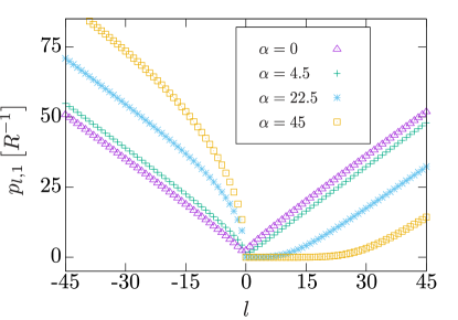
Figure 1: Lowest transverse momentum $p_{l,1}$ as a function of the angular momentum $l$ for various $\alpha$’s.

In Fig. 1 we plot the lowest transverse momentum $p_{l,1}$ as a function of the angular momentum $l$ for various $\alpha$’s corresponding to various magnetic fields $B$ or radius $R$ [see Eq. (13)]. In the $B=0$ case, as shown by the purple triangular points in Fig. 1, positive $l$ modes and negative $(-l-1)$ modes have a degenerated $p_{l,1}$, which is immediately understood from the $\mathcal{CP}$ invariance implying $j\leftrightarrow-j$. Once a finite magnetic field is turned on, however, the momenta for the $l>0$ branch are more suppressed than the $l<0$ branch, as is clear by the green cross, the blue star, and the magenta square points in Fig. 1. Naturally, finite magnetic fields favor a particular direction of the angular momentum and break the $\mathcal{CP}$ invariance. As $\alpha$ increases (i.e., $eB$ or $R$ increases), we see that the lowest momenta become insensitive to $l$ and the conventional Landau zero modes appear .

Figure 1 provides us with more information on the Landau zero modes peculiar to finite-size systems. According to the conventional argument, the Landau degeneracy factor should be given by $\alpha$, but this is no longer the case for a small $\alpha$; we notice in Fig. 1 that $p_{l,1}$ is lifted up from zero at around $l\simeq 10$ for $\alpha=22.5$. This means that there are only half of the Landau zero modes, as compared to the conventional degeneracy factor. We can intuitively understand this as follows. The Landau wave functions with larger $l$’s have a peak position at larger $r$ due to the centrifugal force, which corresponds to a larger Larmor radius of the classical cyclotron motion. The peak width should scale as $1/\sqrt{eB}$. For a large enough $\alpha$, the peak is narrow relative to the system size, and its position hits the boundary at $r=R$ when $l$ reaches $\simeq\alpha$ (which we have numerically confirmed for $\alpha=1000$). For a small $\alpha$, however, the peak is not well localized, so the Landau zero modes are breached before $l$ goes up to $\alpha$. Figure 1 shows a tendency for the degeneracy of the Landau zero modes to approach $\alpha$ with increasing $\alpha$; for $\alpha=45$ the zero modes remain approximately at $l\simeq 30$.

Alternatively, in a slightly different setup of finite-size systems, we can understand the above fact that there emerges less Landau zero modes. We suppose that the system is put not on a cylinder but on a semi-infinite $x-y$ plane with boundary walls at $x=0$ and $x=l_{\text{system}}$. If the Landau gauge $A^{\mu}=(0,-By,0,0)$ is chosen, the peak location of the wave functions is dictated by $p_{x}$. Small momentum modes with $p_{x}\lesssim\pi/l_{B}$ or large momentum modes with $p_{x}\gtrsim\pi/l_{\text{system}}$ receive strong influences from the boundary effect. As a result, for example, a finite-size graphene ribbon under an external magnetic field has energy dispersion spectra with large and small $p_{x}$ modes pushed up, and the Landau zero modes are seen only for intermediate $p_{x}$’s Gusynin et al. (2009).

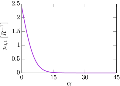
Figure 2: Lowest momentum $p_{0,1}$ (which gives an energy gap) as a function of $\alpha=eBR^{2}/2$.

In Fig. 2 we show a plot for the lowest momentum $p_{0,1}$ as a function of $\alpha$. If there is no boundary, $p_{0,1}$ must be vanishing. For a small $\alpha$, however, a finite gap appears from the boundary effect. This is obviously so because $\alpha\to 0$ implies $B\to 0$ and then there is no Landau quantization. In this particular limit of $\alpha\to 0$, we find that $p_{0,1}$ goes to $2.40483/R$, and this value precisely corresponds to the Bessel zero, $\zeta_{0,1}$, in the discretized momenta (16) for $B=0$ Giordano and Laforgia (1983). We should emphasize that this behavior of $p_{0,1}$ is physically quite important. As argued in Ref. Ebihara et al. (2017), a rotation alone does not change the vacuum structure because the induced effective chemical potential (i.e. the rotational energy shift) is always smaller than the lowest energy gap, $p_{0,1}$. Once $eB$ becomes bigger than the squared system-size inverse (that is, $\alpha\gtrsim 10$ from Fig. 2), however, the energy gap is significantly reduced and the anomalous coupling between the magnetic field and the rotation is then manifested Chen et al. (2016); Hattori and Yin (2016).

IV Integration Measure and Reweighted wave functions

Because the radial momenta are discretized, we replace the transverse momentum integration with the sums over the quantum numbers, $l$ and $k$, i.e.

$$\int\frac{dp_{x}dp_{y}}{(2\pi)^{2}}\longrightarrow\frac{1}{\pi R^{2}}\sum_{l=-\infty}^{\infty}\sum_{k=1}^{\infty}\frac{1}{N_{l,k}^{2}}\;,$$ (18)

where $N_{l,k}$ represents a weight factor which corresponds to the integration measure in finite-size systems. In the $B=0$ case, as discussed in Ref. Ebihara et al. (2017), the weight factor is deduced from the Bessel-Fourier expansion, that is, we know that in the limit of $\alpha\to 0$,

$$\begin{split}N_{l,k}^{2}\;\;\longrightarrow&\;\;\frac{2}{R^{2}}\int_{0}^{R}rdr\,\bigl{[}J_{l}(p_{l,k}r)\bigr{]}^{2}\end{split}$$ (19)

with the discretized momentum $p_{l,k}$ in Eq. (16). From the relation in Eq. (8), we extrapolate the above identification to nonzero $\alpha$ as

$$\begin{split}N_{l,k}^{2}&=\frac{2}{R^{2}}\int_{0}^{R}rdr\,\bigl{[}\Phi_{l}(\lambda_{l,k},\tfrac{1}{2}eBr^{2})\bigr{]}^{2}\\ &=\int_{0}^{1}dx\,\bigl{[}\Phi_{l}(\lambda_{l,k},\alpha x)\bigr{]}^{2}\,.\end{split}$$ (20)

We can easily confirm that the $N_{l,k}$ defined as above satisfies the asymptotic behavior in Eq. (19) in the $\alpha\to 0$ limit. Moreover, we can readily understand that $N_{l,k}^{2}$ goes to $1/\alpha$ in the opposite limit of $\alpha\to\infty$. Then this exactly accounts for the appearance of the Landau degeneracy factor, $\alpha/(\pi R^{2})=eB/(2\pi)$, in Eq. (18) in the strong magnetic field limit, which also validates Eq. (20). Interestingly, as this should be so, we can prove

$$\int_{0}^{1}dx\,\bigl{[}\Phi_{l}(\lambda_{l,k},\alpha x)\bigr{]}^{2}=\int_{0}^{1}dx\,\bigl{[}\Phi_{l+1}(\lambda_{l,k}-1,\alpha x)\bigr{]}^{2}\,.$$ (21)

This is an important relation; thanks to this equality, we can commonly use $N_{l,k}$ to normalize the four component spinors with both $\phi_{l,k}$ and $\varphi_{l,k}$.

As we see in the next section, the propagator involves a spinor matrix that is a product of two wave functions and, in general, $1/N_{l,k}^{2}$ appears together with the propagator. Thus, the physical meaning of $N_{l,k}$ would become more transparent if we define reweighted wave functions by $N_{l,k}$, i.e.,

$$\widetilde{\phi}_{l,k}\equiv\frac{\phi_{l,k}}{\sqrt{\pi R^{2}}N_{l,k}}\,,\qquad\widetilde{\varphi}_{l,k}\equiv\frac{\varphi_{l,k}}{\sqrt{\pi R^{2}}N_{l,k}}$$ (22)

for a certain $R$.

Let us explain the interpretation of the reweighted wave functions, $\widetilde{\phi}_{l,k}$ and $\widetilde{\varphi}_{l,k}$. We solved the Dirac equation and gave definitions for $\phi_{l,k}$ and $\varphi_{l,k}$, but they are not yet properly normalized, where we simply fixed the overall normalization to reproduce the conventional expressions in the limit of no boundary effect. The important point here is that, for $l>0$, $\varphi_{l,k}$ may penetrate outside of $r>R$, while only $\phi_{l,k}$ vanishes at $r=R$; nevertheless, there is no communication across $r=R$ due to the no-flux condition. Therefore, we should normalize the wave functions within $0\leq r\leq R$ only. In other words, we can just presume that the system is empty for $r>R$; owing to the no-flux condition, even in this sharp boundary case, no singularity appears at $r=R$. To avoid confusion, we must stress that the above description is just an interpretation, and the denominator in Eq. (22) is, in any case, uniquely fixed in the replacement of the integration with the discrete sum in Eq. (18).

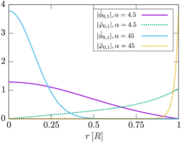
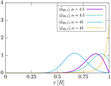
Figure 3: Radial profiles of $|\widetilde{\phi}_{l,1}|$ (the solid lines) and $|\widetilde{\varphi}_{l,1}|$ (dashed lines), which are wave functions normalized by $\sqrt{\pi R^{2}}N_{l,1}$, where all the quantities are given in the unit of $R$. The upper and lower panels show the wave functions for $l=0$ and $l=20$, respectively.

From the point of view of a confined picture of wave functions, the reweighted wave functions, $\widetilde{\phi}_{l,k}$ and $\widetilde{\varphi}_{l,k}$, would make intuitive sense. To see the behavior of the reweighted wave functions, in Fig. 3, we show the radial dependence of $|\widetilde{\phi}_{l,1}|$ and $|\widetilde{\varphi}_{l,1}|$ for $l=0$ (upper panel) and $l=20$ (lower panel) (where we chose $k=1$ to see the lowest modes only). Let us discuss several notable features of the reweighted wave functions below.

First, we focus on the $l=0$ modes, as depicted in the upper panel of Fig. 3. We numerically found $\xi_{0,1}\simeq 0.041$ for a weak magnetic field ($\alpha=4.5$) leading to $N_{0,1}^{2}\simeq 0.19$, and $\xi_{0,1}\simeq 0$ for a stronger magnetic field ($\alpha=45$) leading to $N_{0,1}^{2}\simeq 0.022$. In fact, if $\xi_{0,1}\simeq 0$, as pointed out before, $N_{l,k}^{2}\simeq 1/\alpha$ is a very good approximation.

Because $l=0$ corresponds to the $S$-wave, $|\phi_{0,1}|$ is centered around $r=0$ and becomes more localized for larger $\alpha$’s. As noticed in Eq. (4), on the other hand, $|\varphi_{0,1}|$ has a $l=1$ component of the $P$-wave, so the wave function peaks near the boundary due to the centrifugal force. It is an interesting observation that $|\varphi_{0,1}|$ gets more and more sharply attached to the boundary with increasing $\alpha$. In the infinite size limit $R\to\infty$ (i.e., $\alpha\to\infty$), there is no contribution at all from $|\varphi_{0,1}|$, which means that both $u_{\pm}$ are eigenstates of the spin $s_{z}=\frac{1}{2}\sigma_{z}$ with an eigenvalue $+\frac{1}{2}$, that is, spin-up states. This observation is consistent with the fact that the Landau zero modes have only one spin state.

Next, we consider the $l=20$ modes by looking at the lower panel in Fig. 3. The behavior is qualitatively different from the $l=0$ case. The most nontrivial point is seen in the difference between $|\widetilde{\varphi}_{0,1}|$ in the upper panel and $|\widetilde{\varphi}_{20,1}|$ in the lower panel for $\alpha=4.5$. As explained above, the centrifugal force with $l=1$ pushes $|\widetilde{\varphi}_{0,1}|$ toward $r=R$, and one would expect that such centrifugal effects must be greater for $l=20$. However, $|\widetilde{\phi}_{20,1}|$ is centered rather away from $r=R$, which seems to be quite counterintuitive. We can resolve this puzzle from an indirect constraint from $|\widetilde{\phi}_{l,1}|$; for the $l=0$ case, $|\widetilde{\phi}_{0,1}|$ is not modified much by the boundary because the wave function tail at $r=R$ is negligibly small from the beginning. However, for the $l=20$ case, $|\widetilde{\phi}_{20,1}|$ is significantly distorted and this boundary effect is strong enough to distort $|\widetilde{\varphi}_{20,1}|$ as well.

Another interesting observation for the $l=20$ wave functions is that the spin-up and the spin-down states are not really separable unlike the $l=0$ case. We recall that in the upper panel of Fig. 3 the region with $r<R$ is dominated by $|\widetilde{\phi}_{0,1}|$ only and the wave function inevitably becomes the spin-up eigenstate. In the $l=20$ case, however, due to the centrifugal force, all of the wave functions are shifted in the vicinity of the boundary, and there, $|\widetilde{\phi}_{20,1}|$ and $|\widetilde{\varphi}_{20,1}|$ always coexist; in other words, the Landau degeneracy is violated for large $l$’s, as we already saw in Fig. 2.

We emphasize the importance of the wave function behavior around $r=R$. In this way the wave functions at larger $l$’s are accumulated near $r=R$ and the low-energy dynamics closer to the boundary is more prominently affected by the magnetic background. For instance, as we will confirm in the next section, the dynamical mass enhancement by the magnetic field is further strengthened near the boundary. As a side remark, we note that the mode accumulation around the boundary has no contradiction with the Pauli exclusion principle because all accumulated modes are labeled by different quantum numbers.

V Boundary enhancement of the magnetic catalysis

We will proceed to some concrete calculations to demonstrate the interplay between the magnetic and the surface effects. We will estimate the dynamical mass in the local density approximation using an NJL model. The qualitative features are robust in the sense that it does not depend on a model choice, however, as is clear from the physical discussions in the previous section.

The most fundamental ingredient for concrete calculations is the propagator, $S$, which can be constructed from the solutions (2), (3), (9), and (10). Then, in terms of the Dirac indices, $S$ is a $4\times 4$ matrix whose form is given by

$$\begin{split}&S^{\alpha\beta}(x,x^{\prime})=\ i\int\frac{dp^{0}dp_{z}}{(2\pi)^{2}}\sum_{l=-\infty}^{\infty}\sum_{k=1}^{\infty}\frac{1}{\pi R^{2}N_{l,k}^{2}}\\ &\qquad\times\frac{e^{-ip^{0}(t-t^{\prime})+ip_{z}(z-z^{\prime})}}{(p^{0})^{2}-\varepsilon^{2}+i\epsilon}\mathcal{S}_{l,k}^{\,\alpha\beta}(p;r,\theta,r^{\prime},\theta^{\prime})\,,\end{split}$$ (23)

where the spinor matrix $\mathcal{S}_{l,k}^{\,\alpha\beta}$ in the Dirac representation reads

$$\mathcal{S}_{l,k}(p;r,\theta,r^{\prime},\theta^{\prime})=\begin{pmatrix}\mathcal{M}_{l,k}^{(+)}&\mathcal{N}_{l,k}^{(+)}\\ \mathcal{N}_{l,k}^{(-)}&\mathcal{M}_{l,k}^{(-)}\end{pmatrix}$$ (24)

with

$$\begin{split}\mathcal{M}_{l,k}^{(\pm)}&\equiv\begin{pmatrix}(\pm p_{0}+m)\phi_{l,k}\phi^{\prime}_{l,k}&0\\ 0&(\pm p_{0}+m)\varphi_{l,k}\varphi^{\prime}_{l,k}\end{pmatrix}\,,\\ \mathcal{N}_{l,k}^{(\pm)}&\equiv\begin{pmatrix}-p_{z}\phi_{l,k}\phi^{\prime}_{l,k}&\pm i\sqrt{2eB\lambda_{l,k}}\phi_{l,k}\varphi^{\prime}_{l,k}\\ \mp i\sqrt{2eB\lambda_{l,k}}\varphi_{l,k}\phi^{\prime}_{l,k}&p_{z}\varphi_{l,k}\varphi^{\prime}_{l,k}\end{pmatrix}\,.\end{split}$$ (25)

In the above equations, we use a short notation for the wave functions; $\phi_{l,k}=\phi_{l,k}(r,\theta)$, $\phi^{\prime}_{l,k}=\phi_{l,k}^{*}(r^{\prime},\theta^{\prime})$, $\varphi_{l,k}=\varphi_{l,k}(r,\theta)$, and $\varphi^{\prime}_{l,k}=\varphi_{l,k}^{*}(r^{\prime},\theta^{\prime})$. We note that $\pi R^{2}N_{l,k}^{2}$ in Eq. (23) may have been absorbed into redefinition of $\phi_{l,k}\to\widetilde{\phi}_{l,k}$ and $\varphi_{l,k}\to\widetilde{\varphi}_{l,k}$.

To study the boundary effect for the dynamical mass generation associated with the spontaneous breaking of chiral symmetry, we analyze the NJL model whose Lagrangian density is

$$\mathcal{L}=\bar{\psi}\,i\gamma^{\mu}(\partial_{\mu}+ieA_{\mu})\psi+\frac{G}{2}\bigl{[}(\bar{\psi}\psi)^{2}+(\bar{\psi}i\gamma_{5}\psi)^{2}\bigr{]}\;.$$ (26)

In the mean-field approximation (which is justified when there are infinitely many fermion species), the gap equation or the condition to minimize the thermodynamic potential is written as

$$m=G\,\text{tr}[S(x,x)]\,.$$ (27)

Since translation invariance is lost along the radial direction, the dynamical mass has the $r$ dependence, and thus we should regard Eq. (27) as a functional equation to determine a function $m(r)$. It is, however, numerically demanding to solve this functional equation self-consistently. Besides, our present purpose is not to quantify the effects but to demonstrate robust features of the surface effects. Thus, we reasonably simplify the problem by employing the local density approximation under an assumption of $|\partial_{r}m(r)|\ll m(r)^{2}$ Jiang and Liao (2016). Then, we can approximately treat the energy dispersion relation as simple as $\varepsilon(r)=\sqrt{2eB\lambda_{l,k}+p_{z}^{2}+m(r)^{2}}$. Utilizing Eq. (23) and inserting a ultraviolet regulator, we write the explicit form of the gap equation as

$$\begin{split}\frac{m(r)}{G}&=m(r)\int_{-\infty}^{\infty}\frac{dp_{z}}{2\pi}\sum_{l=-\infty}^{\infty}\sum_{k=1}^{\infty}\frac{f(p\,;\Lambda,\delta\Lambda)}{\pi R^{2}N_{l,k}^{2}}\\ &\times\frac{\bigl{[}\Phi_{l}(\lambda_{l,k},\tfrac{1}{2}eBr^{2})\bigr{]}^{2}+\bigl{[}\Phi_{l+1}(\lambda_{l,k}-1,\tfrac{1}{2}eBr^{2})\bigr{]}^{2}}{\varepsilon(r)}\,.\end{split}$$ (28)

Here, we note that the choice of the ultraviolet regulator is a part of the model definition, and in our numerical calculations presented below, we adopt a smooth 3-momentum cutoff function as follows Chen et al. (2016):

$$f(p\,;\Lambda,\delta\Lambda)=\frac{\sinh(\Lambda/\delta\Lambda)}{\cosh(p/\delta\Lambda)+\cosh(\Lambda/\delta\Lambda)}$$ (29)

with $p=\sqrt{2eB\lambda_{l,k}+p_{z}^{2}}$. To discuss the magnetic catalysis, the proper-time regularization Schwinger (1951) and the Pauli-Villars regularization would be a common choice in NJL model studies (see e.g., see Ref. Klimenko (1992a); Gusynin et al. (1994)). It is, however, known that a naive momentum cutoff with a step function could also give a qualitatively correct result, as long as the smearing parameter $\delta\Lambda$ is not too small Gorbar et al. (2011). Therefore, the above simple $f(p;\Lambda,\delta\Lambda)$ value should suffice for our present purpose of qualitative analysis. For the numerical calculation we chose the model parameters as

$$G=24\,\Lambda^{-2}\,,\qquad\delta\Lambda=0.05\,\Lambda\,.$$ (30)

Here, we can trivially scale out $\Lambda$ by measuring all of the quantities in units of $\Lambda$. Also we fix the system size to be

$$R=30\,\Lambda^{-1}\,.$$ (31)

This value itself is not relevant for our discussions. For $\Lambda\simeq 1\,\text{GeV}$ (that is, a QCD scale), the above choice of the system size $R=30\,\Lambda^{-1}$ corresponds to the typical radial scale of heavy ions, $R\simeq 6\,\text{fm}$. In units of $\Lambda$, in this model with $B=0$ and $R\to\infty$, the critical coupling is

$$G_{c}=19.58\,\Lambda^{-2}\,,$$ (32)

which is smaller than the present $G$.

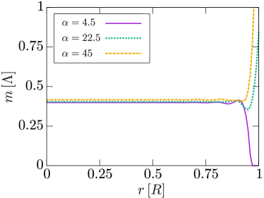
Figure 4: Dynamical mass as a function of the radial coordinate $r$ for the choice of $R=30\Lambda^{-1}$. Near the boundary the dynamical mass rapidly increases due to the accumulation of the boundary modes.

In Fig. 4 we show the dynamical mass $m(r)$ solved from the gap equation in the local density approximation. We see from Fig. 4 that the magnetic field effect is minor for $\alpha=4.5$. The $r$ dependence of the dynamical mass is flat up to $r\simeq 0.7R$, and $m(r)$ becomes oscillatory for $r\gtrsim 0.7R$. Such oscillation results from the boundary effect, and its exact form depends on the regularization $f(p;\Lambda,\delta\Lambda)$ as well as the system size. Actually, for a larger $R$, the discretized momentum spacing is smaller (which is $\propto 1/R$), and thus the oscillating period should be smaller accordingly. For the even larger $r\simeq R$, the dynamical mass eventually vanishes. This oscillating and vanishing behavior of $m(r)$ is quite similar to what is observed in the $B=0$ case (see Fig. 1 in Ref. Ebihara et al. (2017)). We also comment on the validity of the local density approximation. The required condition, $|\partial_{r}m(r)|\ll m(r)^{2}$ is satisfied for almost all $r$’s except the region very close to $R$.

In contrast to $\alpha=4.5$, the dynamical mass behavior for stronger magnetic fields ($\alpha=22.5$ and $45$ in Fig. 4) is qualitatively different. As long as $r$ is away from the boundary, a flat plateau continues, until oscillations appear around $r\simeq 0.7R$. Then, $m(r)$ does not vanish but is pushed up as $r$ approaches $R$. This abnormally enhanced magnetic catalysis (called the surface magnetic catalysis in this work) is a consequence of the interplay between the magnetic field and the boundary effect.

We shall explain how to understand the surface magnetic catalysis in terms of the wave functions. We have already seen that the spin-down mixture by $\widetilde{\varphi}_{l,k}$ piles up near $r\simeq R$ for a large $l$, as shown in the lower panel of Fig. 3. If there were no boundary, the peak position of the wave functions with large $l$ would be at a far distance. However, in the presence of the boundary at $r=R$, these modes, which would have no contribution without a boundary, come to make a finite contribution near $r\simeq R$. Then, the gap equation (28) receives a contribution of spin-down boundary modes with various $l$’s. We could say, in other words, that the surface magnetic catalysis is induced by the combination of the incomplete spin alignment of the Landau levels seen in Sec. III and the reweighting factor from the integration measure argued for in Sec. IV.

VI Conclusion

In this paper, imposing a proper boundary condition in terms of the fermionic flux (the same conclusion can be drawn from the Hermiticity of the Hamiltonian), we analyzed the finite-size effect on fermionic matter coupled with an external magnetic field. We obtained incomplete or nondegenerate Landau levels; that is, for states with larger angular momenta relative to the system size, the Landau quantized spectra are not degenerate. Also, we noticed that the spin-up and spin-down structures of the wave functions are significantly changed by the finite-size effect. In the thermodynamic limit of infinite volume, only the spin-up modes (if the magnetic field is positive along the quantum axis of the angular momentum) occupy the Landau zero modes, and the spin-down modes become irrelevant because the spin-down modes are tightly localized in the vicinity of the boundary at an infinitely great distance. In finite-size systems, however, the magnetic field partially overcomes this spin separation and forms the gapless Landau zero modes for both spin-up and spin-down states. This pairwise structure of spin-up modes in the bulk and spin-down modes at the surface is quite remarkable for magnetic phenomena related to chirality imbalance. For instance, in finite-size systems, even though an anomalous fermionic current density is nonzero in bulk, the whole current would vanish together with the surface contribution kam .

In this paper, we found a novel aspect of the magnetic catalysis peculiar to finite-size systems; the catalyzing effect on the dynamical mass is more intense in the vicinity of the boundary, which is called the surface magnetic catalysis in this work. Because the surface magnetic catalysis shows a sharp enhancement of the dynamical mass at the surface, strictly speaking, we must say that the local density approximation, in which spatial derivatives of the dynamical mass are neglected, adopted in the present work might be not reliable enough. We must stress, however, that the origin of such a strong enhancement can be explained by the accumulation of many spin-down zero modes near the boundary, which does not rely on any model or approximation. Therefore, even including the higher order derivative terms of the dynamical mass, nothing qualitative should be changed. Regardless of the model or the approximation, similar spatial profile of the dynamical mass or the condensate must be reproduced. Furthermore, we note that the geometrical shape of the boundary is not relevant to the accumulation of the low-energy modes. Hence, lattice numerical simulations could test the surface magnetic catalysis in a realistic finite-size system (for instance, graphene DeTar et al. (2016); *DeTar:2016dmj) if not the periodic boundary condition but an appropriate no-flux boundary condition is formulated in terms of the link variables.

The findings in this paper have various applications. For Dirac and Weyl semimetals we expect fruitful phase structures from the proper treatment of the finite-size effect. In Ref. Gorbar et al. (2013), the authors argue that an external magnetic field leads to the dynamical transformation from a Dirac semimetal (a state without the chiral shift Gorbar et al. (2009)) to a Weyl semimetal (a state with the chiral shift). This is the case for large systems. According to our result, the magnetic property of the boundary should differ from that of the bulk, and thus it would be intriguing to revisit the possibility of the dynamical transformation including the surface effect.

Another interesting extension is the coupling to rotation. For instance, the anomalous coupling with the magnetic field and the rotation Ebihara et al. (2017); Hattori and Yin (2016) should lead to a fascinating effect on the energy-momentum tensor of a quark-gluon plasma Hernandez and Kovtun (2017); mam . Besides, the interplay between the magnetic field and the rotation should influence the dynamical symmetry breaking and the equation of state. As discussed in Ref. Chen et al. (2016), in rotating matter, the magnetic catalysis and the inverse magnetic catalysis are driven, respectively, by small and large rotational effects. At a short distance $r$ from the rotational center, the magnetic catalysis is realized because the centrifugal force, which is proportional to $r$, is still small. Since the edge region near the boundary is heavily affected by the magnetic field, on the other hand, it is nontrivial whether the inverse magnetic catalysis really takes place around the boundary once the results in Ref. Chen et al. (2016) are augmented by the finite-size effects. The quantitative details of the chiral structure in magnetized rotating systems deserve further investigations, and we will report our progress in forthcoming papers.

Appendix A Solving the Dirac equation

We derive the solutions (2), (3), (9), and (10). The Dirac equation for fermions confined in a finite-size system under an external magnetic field is given by

$$(i\gamma^{\mu}D_{\mu}-m)\psi=0\,,$$ (33)

where $D_{\mu}=\partial_{\mu}+ieA_{\mu}$ is the covariant derivative with the symmetric gauge $A^{\mu}=(0,-By/2,Bx/2,0)$. Multiplying $(i\gamma^{\nu}D_{\nu}+m)$ by the above Dirac equation and changing to the cylindrical coordinates, we can rewrite Eq. (1) as follows:

$$\begin{split}&\Biggl{[}-\partial_{t}^{2}+\partial_{z}^{2}-m^{2}+\partial_{r}^{2}+\frac{1}{r}\partial_{r}+\frac{1}{r^{2}}\partial_{\theta}^{2}\\ &\qquad+eB(-i\partial_{\theta}+\sigma^{12})-\biggl{(}\frac{eBr}{2}\biggr{)}^{2}\ \Biggr{]}\psi=0\,.\end{split}$$ (34)

with $\sigma^{12}=\tfrac{i}{2}[\gamma^{1},\gamma^{2}]=\text{diag}(\sigma_{z},\sigma_{z})$. Since the $t$- and $z$-dependent terms are separately solved in the form of plane waves, we can parametrize two linear independent solutions with positive energy as

$$\psi=u_{\pm}=e^{-i\varepsilon t+ip_{z}z}\begin{pmatrix}f_{1\pm}(r,\theta)\\ f_{2\pm}(r,\theta)\end{pmatrix}\,,$$ (35)

where $\pm$ refers to different polarizations.

Let us first focus on $f_{1\pm}$. While the total angular momentum, $\hat{J}_{z}=\hat{L}_{z}+\hat{S}_{z}=-i\partial_{\theta}+\tfrac{1}{2}\sigma^{12}$, is a good quantum number in the present system, neither $\hat{L}_{z}$ nor $\hat{S}_{z}$ is. For this reason it is convenient to choose $u_{\pm}$ as an eigenstate of $\hat{J}_{z}$ with its common eigenvalue denoted by $j$. We here employ the Dirac representation for $\gamma^{\mu}$’s, i.e.,

$$\gamma^{0}=\begin{pmatrix}1&0\\ 0&-1\end{pmatrix}\,,\qquad\gamma^{i}=\begin{pmatrix}0&\sigma^{i}\\ -\sigma^{i}&0\end{pmatrix}\,.$$ (36)

Then, we fix the angular part of the two component function $f_{1\pm}$ as

$$f_{1\pm}(r,\theta)=e^{il_{\pm}\theta}\tilde{f}_{1\pm}(r)\chi_{\pm}$$ (37)

with $\sigma_{z}\chi_{\pm}=\pm\chi_{\pm}$ and $l_{+}+1/2=l_{-}-1/2=j$. From Eq. (34) we find the equation of motion for the radial part, $\tilde{f}_{1\pm}$, which reads

$$\begin{split}&\Biggl{[}\partial_{r}^{2}+\frac{1}{r}\partial_{r}-\frac{l_{\pm}^{2}}{r^{2}}+2eB\lambda_{l,k}\\ &\qquad\qquad+eB(l_{\pm}\pm 1)-\biggl{(}\frac{eBr}{2}\biggr{)}^{2}\ \Biggr{]}\tilde{f}_{1\pm}=0\end{split}$$ (38)

with the dispersion relation,

$$2eB\lambda_{l,k}=\varepsilon^{2}-p_{z}^{2}-m^{2}\,.$$ (39)

Using the scalar function $\Phi_{l}(\lambda,\tfrac{1}{2}eBr^{2})$ defined in Eqs. (5) and (7), we identify the solutions for this equation as $\tilde{f}_{1+}=\Phi_{l}(\lambda_{l,k},\tfrac{1}{2}eBr^{2})$ and $\tilde{f}_{1-}=\Phi_{l+1}(\lambda_{l,k}-1,\tfrac{1}{2}eBr^{2})$, where we introduce the quantum number for $\hat{L}_{z}$,

$$l\equiv j-1/2\,,\quad\text{i.e.\ }\quad l=l_{+}=l_{-}-1\,.$$ (40)

Thus, we find that $f_{1\pm}$ is represented as follows:

$$f_{1+}(r,\theta)=\phi_{l,k}\chi_{+}\,,\qquad f_{1-}(r,\theta)=\varphi_{l,k}\chi_{-}\,,$$ (41)

with $\phi_{l,k}$ and $\varphi_{l,k}$ in Eq. (4).

Also, we can solve the lower components $f_{2\pm}$ from

$$(\varepsilon+m)f_{2\pm}=(-i{\boldsymbol{\sigma}}_{\perp}\cdot{\boldsymbol{D}}_{\perp}+\sigma_{z}p_{z})f_{1\pm}\,,$$ (42)

which follows from the Dirac equation in the Dirac representation. In the cylindrical coordinates, the covariant derivative term, $-i{\boldsymbol{\sigma}}_{\perp}\cdot{\boldsymbol{D}}_{\perp}$, is represented as

$$-i{\boldsymbol{\sigma}}_{\perp}\cdot{\boldsymbol{D}}_{\perp}=\begin{pmatrix}0&a^{\dagger}\\ a&0\end{pmatrix}\,,$$ (43)

where we introduce the ladder operators defined by

$$\begin{split}a&\equiv-ie^{i\theta}(\partial_{r}+ir^{-1}\partial_{\theta}+eBr/2)\,,\\ a^{\dagger}&\equiv-ie^{-i\theta}(\partial_{r}-ir^{-1}\partial_{\theta}-eBr/2)\,.\\ \end{split}$$ (44)

In fact, we can explicitly check to see that $a$ and $a^{\dagger}$ act as the ladder operator on $\phi_{l,k}$ and $\varphi_{l,k}$:

$$\begin{split}&a\phi_{l,k}=i\sqrt{2eB\lambda_{l,k}}\varphi_{l,k}\,,\\ &a^{\dagger}\varphi_{l,k}=-i\sqrt{2eB\lambda_{l,k}}\phi_{l,k}\,.\end{split}$$ (45)

From these relations and the explicit form of $\tilde{f}_{1\pm}$, we can solve Eq. (42) for $f_{2\pm}$ as

$$\begin{split}f_{2+}&=\frac{p_{z}}{\varepsilon+m}\phi_{l,k}\chi_{+}+\frac{i\sqrt{2eB\lambda_{l,k}}}{\varepsilon+m}\varphi_{l,k}\chi_{-}\,,\\ f_{2-}&=\frac{-i\sqrt{2eB\lambda_{l,k}}}{\varepsilon+m}\phi_{l,k}\chi_{+}+\frac{-p_{z}}{\varepsilon+m}\varphi_{l,k}\chi_{-}\,,\end{split}$$ (46)

which finally amounts to Eqs. (2) and (3) for the positive-energy solution.

In the same way, we find the negative-energy solution, $v_{\pm}$. We suppose that the solution takes the following form:

$$\psi=v_{\pm}=e^{i\varepsilon t-ip_{z}z}\begin{pmatrix}g_{1\mp}(r,\theta)\\ g_{2\mp}(r,\theta)\end{pmatrix}$$ (47)

with

$$g_{2+}(r,\theta)=\varphi_{l,k}\chi_{+}\,,\qquad g_{2-}(r,\theta)=-\phi_{l,k}\chi_{-}\,.$$ (48)

Then, the Dirac equation fixes the form of the upper component $g_{1\pm}$ through

$$(\varepsilon+m)g_{1\pm}=(i{\boldsymbol{\sigma}}_{\perp}\cdot{\boldsymbol{D}}_{\perp}-\sigma_{z}p_{z})g_{2\pm}\,.$$ (49)

We can explicitly solve this equation, leading to

$$\begin{split}g_{1+}&=\frac{-p_{z}}{\varepsilon+m}\phi_{l,k}\chi_{+}+\frac{-i\sqrt{2eB\lambda_{l,k}}}{\varepsilon+m}\varphi_{l,k}\chi_{-}\,,\\ g_{1-}&=\frac{-i\sqrt{2eB\lambda_{l,k}}}{\varepsilon+m}\phi_{l,k}\chi_{+}+\frac{-p_{z}}{\varepsilon+m}\varphi_{l,k}\chi_{-}\,.\end{split}$$ (50)

Hence, we obtain Eqs. (9) and (10).

References

- Cheng and Olinto (1994) B.-l. Cheng and A. V. Olinto, Phys. Rev. D50, 2421 (1994).
- Baym et al. (1996) G. Baym, D. Bodeker, and L. D. McLerran, Phys. Rev. D53, 662 (1996), arXiv:hep-ph/9507429 [hep-ph] .
- Grasso and Rubinstein (2001) D. Grasso and H. R. Rubinstein, Phys. Rept. 348, 163 (2001), arXiv:astro-ph/0009061 [astro-ph] .
- Duncan and Thompson (1992) R. C. Duncan and C. Thompson, Astrophys. J. 392, L9 (1992).
- Skokov et al. (2009) V. Skokov, A. Yu. Illarionov, and V. Toneev, Int. J. Mod. Phys. A24, 5925 (2009), arXiv:0907.1396 [nucl-th] .
- Voronyuk et al. (2011) V. Voronyuk, V. D. Toneev, W. Cassing, E. L. Bratkovskaya, V. P. Konchakovski, and S. A. Voloshin, Phys. Rev. C83, 054911 (2011), arXiv:1103.4239 [nucl-th] .
- Deng and Huang (2012) W.-T. Deng and X.-G. Huang, Phys. Rev. C85, 044907 (2012), arXiv:1201.5108 [nucl-th] .
- Fukushima et al. (2008) K. Fukushima, D. E. Kharzeev, and H. J. Warringa, Phys. Rev. D78, 074033 (2008), arXiv:0808.3382 [hep-ph] .
- Son and Surowka (2009) D. T. Son and P. Surowka, Phys. Rev. Lett. 103, 191601 (2009), arXiv:0906.5044 [hep-th] .
- Kharzeev et al. (2016) D. E. Kharzeev, J. Liao, S. A. Voloshin, and G. Wang, Prog. Part. Nucl. Phys. 88, 1 (2016), arXiv:1511.04050 [hep-ph] .
- Huang (2016) X.-G. Huang, Rept. Prog. Phys. 79, 076302 (2016), arXiv:1509.04073 [nucl-th] .
- Klimenko (1992a) K. G. Klimenko, Z. Phys. C54, 323 (1992a).
- Klimenko (1992b) K. G. Klimenko, Theor. Math. Phys. 90, 1 (1992b).
- Gusynin et al. (1994) V. P. Gusynin, V. A. Miransky, and I. A. Shovkovy, Phys. Rev. Lett. 73, 3499 (1994), [Erratum: Phys. Rev. Lett.76,1005(1996)], arXiv:hep-ph/9405262 [hep-ph] .
- Gusynin et al. (1996) V. P. Gusynin, V. A. Miransky, and I. A. Shovkovy, Nucl. Phys. B462, 249 (1996), arXiv:hep-ph/9509320 [hep-ph] .
- Fraga and Mizher (2008) E. S. Fraga and A. J. Mizher, Phys. Rev. D78, 025016 (2008), arXiv:0804.1452 [hep-ph] .
- Mizher et al. (2010) A. J. Mizher, M. N. Chernodub, and E. S. Fraga, Phys. Rev. D82, 105016 (2010), arXiv:1004.2712 [hep-ph] .
- Andersen and Khan (2012) J. O. Andersen and R. Khan, Phys. Rev. D85, 065026 (2012), arXiv:1105.1290 [hep-ph] .
- Ferrari et al. (2012) G. N. Ferrari, A. F. Garcia, and M. B. Pinto, Phys. Rev. D86, 096005 (2012), arXiv:1207.3714 [hep-ph] .
- Fraga and Palhares (2012) E. S. Fraga and L. F. Palhares, Phys. Rev. D86, 016008 (2012), arXiv:1201.5881 [hep-ph] .
- Bali et al. (2012a) G. S. Bali, F. Bruckmann, G. Endrodi, Z. Fodor, S. D. Katz, S. Krieg, A. Schafer, and K. K. Szabo, JHEP 02, 044 (2012a), arXiv:1111.4956 [hep-lat] .
- Bali et al. (2012b) G. S. Bali, F. Bruckmann, G. Endrodi, Z. Fodor, S. D. Katz, and A. Schafer, Phys. Rev. D86, 071502 (2012b), arXiv:1206.4205 [hep-lat] .
- Bruckmann et al. (2013) F. Bruckmann, G. Endrodi, and T. G. Kovacs, JHEP 04, 112 (2013), arXiv:1303.3972 [hep-lat] .
- Johnson and Kundu (2008) C. V. Johnson and A. Kundu, JHEP 12, 053 (2008), arXiv:0803.0038 [hep-th] .
- Hong et al. (1996) D. K. Hong, Y. Kim, and S.-J. Sin, Phys. Rev. D54, 7879 (1996), arXiv:hep-th/9603157 [hep-th] .
- Skokov (2012) V. Skokov, Phys. Rev. D85, 034026 (2012), arXiv:1112.5137 [hep-ph] .
- Scherer and Gies (2012) D. D. Scherer and H. Gies, Phys. Rev. B85, 195417 (2012), arXiv:1201.3746 [cond-mat.str-el] .
- Andersen and Tranberg (2012) J. O. Andersen and A. Tranberg, JHEP 08, 002 (2012), arXiv:1204.3360 [hep-ph] .
- Fukushima and Pawlowski (2012) K. Fukushima and J. M. Pawlowski, Phys. Rev. D86, 076013 (2012), arXiv:1203.4330 [hep-ph] .
- Kamikado and Kanazawa (2014) K. Kamikado and T. Kanazawa, JHEP 03, 009 (2014), arXiv:1312.3124 [hep-ph] .
- Hattori et al. (2017) K. Hattori, K. Itakura, and S. Ozaki, (2017), arXiv:1706.04913 [hep-ph] .
- Shovkovy (2013) I. A. Shovkovy, Lect. Notes Phys. 871, 13 (2013), arXiv:1207.5081 [hep-ph] .
- Miransky and Shovkovy (2015) V. A. Miransky and I. A. Shovkovy, Phys. Rept. 576, 1 (2015), arXiv:1503.00732 [hep-ph] .
- Ebert et al. (1999) D. Ebert, K. G. Klimenko, M. A. Vdovichenko, and A. S. Vshivtsev, Phys. Rev. D61, 025005 (1999), arXiv:hep-ph/9905253 [hep-ph] .
- Preis et al. (2011) F. Preis, A. Rebhan, and A. Schmitt, JHEP 03, 033 (2011), arXiv:1012.4785 [hep-th] .
- Preis et al. (2013) F. Preis, A. Rebhan, and A. Schmitt, Lect. Notes Phys. 871, 51 (2013), arXiv:1208.0536 [hep-ph] .
- Fukushima and Hidaka (2013) K. Fukushima and Y. Hidaka, Phys. Rev. Lett. 110, 031601 (2013), arXiv:1209.1319 [hep-ph] .
- Chen et al. (2016) H.-L. Chen, K. Fukushima, X.-G. Huang, and K. Mameda, Phys. Rev. D93, 104052 (2016), arXiv:1512.08974 [hep-ph] .
- Liang and Wang (2005) Z.-T. Liang and X.-N. Wang, Phys. Rev. Lett. 94, 102301 (2005), [Erratum: Phys. Rev. Lett.96,039901(2006)], arXiv:nucl-th/0410079 [nucl-th] .
- Huang et al. (2011) X.-G. Huang, P. Huovinen, and X.-N. Wang, Phys. Rev. C84, 054910 (2011), arXiv:1108.5649 [nucl-th] .
- Becattini et al. (2015) F. Becattini, G. Inghirami, V. Rolando, A. Del Zanna, L. De Pace, G. Pagliara, and V. Chandra, Eur. Phys. J. C75, 406 (2015), arXiv:1501.04468 [nucl-th] .
- Jiang et al. (2016) Y. Jiang, Z.-W. Lin, and J. Liao, Phys. Rev. C94, 044910 (2016), arXiv:1602.06580 [hep-ph] .
- Aristova et al. (2016) A. Aristova, D. Frenklakh, A. Gorsky, and D. Kharzeev, JHEP 10, 029 (2016), arXiv:1606.05882 [hep-ph] .
- Deng and Huang (2016) W.-T. Deng and X.-G. Huang, Phys. Rev. C93, 064907 (2016), arXiv:1603.06117 [nucl-th] .
- Davies et al. (1996) P. C. W. Davies, T. Dray, and C. A. Manogue, Phys. Rev. D53, 4382 (1996), arXiv:gr-qc/9601034 [gr-qc] .
- Ambrus and Winstanley (2016) V. E. Ambrus and E. Winstanley, Phys. Rev. D93, 104014 (2016), arXiv:1512.05239 [hep-th] .
- Ebihara et al. (2017) S. Ebihara, K. Fukushima, and K. Mameda, Phys. Lett. B764, 94 (2017), arXiv:1608.00336 [hep-ph] .
- Jiang and Liao (2016) Y. Jiang and J. Liao, Phys. Rev. Lett. 117, 192302 (2016), arXiv:1606.03808 [hep-ph] .
- Chernodub and Gongyo (2017a) M. N. Chernodub and S. Gongyo, JHEP 01, 136 (2017a), arXiv:1611.02598 [hep-th] .
- Chernodub and Gongyo (2017b) M. N. Chernodub and S. Gongyo, Phys. Rev. D95, 096006 (2017b), arXiv:1702.08266 [hep-th] .
- Chernodub and Gongyo (2017c) M. N. Chernodub and S. Gongyo, (2017c), arXiv:1706.08448 [hep-th] .
- Hattori and Yin (2016) K. Hattori and Y. Yin, Phys. Rev. Lett. 117, 152002 (2016), arXiv:1607.01513 [hep-th] .
- Buchholz (2013) H. Buchholz, The confluent hypergeometric function: with special emphasis on its applications, Vol. 15 (Springer Science & Business Media, 2013).
- (54) Y, Hidaka, private communications.
- Note (1) More precisely, this is not exactly a gapless mode but rather a “pseudo” zero mode, and the exact one is produced in the limit of , as seen in Fig. 2.
- Gusynin et al. (2009) V. P. Gusynin, V. A. Miransky, S. G. Sharapov, I. A. Shovkovy, and C. M. Wyenberg, Physical Review B 79, 115431 (2009), arXiv:0801.0708 [cond-mat.mes-hall] .
- Giordano and Laforgia (1983) C. Giordano and A. Laforgia, Journal of Computational and Applied Mathematics 9, 221 (1983).
- Schwinger (1951) J. S. Schwinger, Phys. Rev. 82, 664 (1951).
- Gorbar et al. (2011) E. V. Gorbar, V. A. Miransky, and I. A. Shovkovy, Phys. Rev. D83, 085003 (2011), arXiv:1101.4954 [hep-ph] .
- (60) K. Hattori, X.-G. Huang, Y. Hidaka, and S. Kamata, in preparation.
- DeTar et al. (2016) C. DeTar, C. Winterowd, and S. Zafeiropoulos, Phys. Rev. Lett. 117, 266802 (2016), arXiv:1607.03137 [hep-lat] .
- DeTar et al. (2017) C. DeTar, C. Winterowd, and S. Zafeiropoulos, Phys. Rev. B95, 165442 (2017), arXiv:1608.00666 [hep-lat] .
- Gorbar et al. (2013) E. V. Gorbar, V. A. Miransky, and I. A. Shovkovy, Phys. Rev. B88, 165105 (2013), arXiv:1307.6230 [cond-mat.mes-hall] .
- Gorbar et al. (2009) E. V. Gorbar, V. A. Miransky, and I. A. Shovkovy, Phys. Rev. C80, 032801 (2009), arXiv:0904.2164 [hep-ph] .
- Hernandez and Kovtun (2017) J. Hernandez and P. Kovtun, JHEP 05, 001 (2017), arXiv:1703.08757 [hep-th] .
- (66) K. Hattori, X.-G. Huang, and K. Mameda, in preparation.