Determination and biological application of a time dependent thermal parameter and sensitivity analysis for a conduction problem with superficial evaporation
Abstract
A boundary value problem, which could represent a transcendent temperature conduction problem with evaporation in a part of the boundary, was studied to determine unknown thermophysical parameters, which can be constants or time dependent functions. The goal of this paper was elucidate which parameters may be determined using only the measured superficial temperature in part of the boundary of the domain. We formulated a nonlinear inverse problem to determine the unknown parameters and a sensitivity analysis was also performed. In particular, we introduced a new way of computing a sensitivity analysis of a parameter which is variable in time. We applied the proposed method to model tissue temperature changes under transient conditions in a biological problem: the hamster cheek pouch. In this case, the time dependent unknown parameter can be associated to the loss of heat due to water evaporation at the superficial layer of the pouch. Finally, we performed the sensitivity analysis to determine the most sensible parameters to variations of the superficial experimental data in the hamster cheek pouch.
Keywords: Boundary value problem, Determination of parameters, Sensitivity analysis, Hamster cheek pouch.
1 Introduction
Diffusion problems have been studied in many different areas, such as heat conduction [1], sediment transport in a river [2], the study of the weather [3], or in drying food technology [4, 5, 6]. The heat transport in a certain object may be modeled through a convection-diffusion differential equation. The boundary conditions usually considered are: a constant temperature (Dirichlet condition), a fixed heat flux (Neumann condition) or a mixed condition, where the heat flux depends on the temperature at the boundary.
In [7] some thermal inverse problems were considered in a mathematical tumor model. They estimated simultaneously unknown thermophysical and geometrical parameters, through an evolutionary algorithm. All the parameters were constants and no evaporation was considered. In [8] a space-dependent convection parameter was determined through a nonlinear least squares technique, using several temperature measurements at different times in different locations of the domain. In [9], we observed that exophytic tumors and irradiated tissues, principally those with ulcers, exhibit mass moisture transfer in the tissue-air interphase.
In this work, we resolved a partial differential problem considering a time-dependent extra term in the mixed condition, which can be associated with a loss of heat due to superficial evaporation. Having measurements of temperature in a section of a particular domain during time, a nonlinear inverse problem was formulated to determine some thermophysical parameters such as the superficial heat loss or the heat conductivity. A sensitivity analysis was also performed. Finally the parameter determination and the sensitivity analysis were validated using our previous study on tissue temperature responses in the hamster cheek pouch [9].
2 Description of the conduction problem
Let us consider a one dimensional spatial domain , and the following boundary value problem:
| (1a) | ||||
| (1b) | ||||
| (1c) | ||||
| (1d) | ||||
where are real constants, and are real functions, and 222We chose one spatial dimension for simplicity. This procedure can be easily extended to more dimensions without loss of generality..
In general, the parameters , and are fundamental in using this type of differential equation problem with boundary conditions given by Eqs. (1b), (1c) and (1d). Note that Eq. (1b) includes a time-dependent parameter, , which is defined only in the boundary . In particular, are often approximated, and sometimes their values are just guessed. If there is an experimental measure of the temperature on the boundary , an inverse problem can be formulated defining the following cost function:
| (2) |
where is the measured superficial temperature. Therefore, some parameters can be determined minimizing the cost function .
The goal of this paper is to find which parameters may be determined using only the measured superficial temperature. First we proposed a method to identify the function such that the solution of the problem (1) minimizes the cost function (Section 3). Then, we introduced a new way of computing a sensitivity analysis of a variable parameter (Section 4). As an example, in Section 5, we applied this problem to model tissue temperature changes, under transient conditions, in the hamster cheek pouch. In this biological problem, the function can be associated to the loss of heat due to water evaporation at the superficial layer of the cheek pouch. Finally, we performed the sensitivity analysis to determine the most sensible parameters to variations of the superficial experimental data (Section 5.3).
3 Determination of the function
The goal of this section is to determine the function , assuming that the rest of the parameters are known constant. To solve the direct problem (1) we used the Finite Element Method (FEM), meshed the spatial-time333The mesh used is a triangular uniform mesh, where the nodes are obtained by the Cartesian product of a discretization in time and a discretization in space. Using polynomials of degree one and this particular mesh makes the FEM equivalent to a finite difference scheme. domain and obtained the triangulation . We define the following finite element spaces:
| (3) |
| (4) |
| (5) |
The weak formulation of problem (1) is the following:
where,
| (6) | |||
| (7) |
Let be the nodes of the triangulation , and be the subset of index whose nodes are in the boundary . We define the function as follows,
where is the base of the space .
The inverse problem of determining consists in obtaining the values of such that the solution of the weak formulation problem is close to the measured temperatures. Let be a solution of . The cost function can be approximated by:
We defined the following optimization problem:
-
Find such that minimizes the cost function , where is a solution of using the values of to define .
We used the Lagrange Method to determine the variation of by each , and obtaining a direction of descent. Suppose that for the values of are fixed, and we vary only the parameter . We define the following function:
| (8) |
where y is defined in (6) and (7), and the subscript means that we are using in the fixed values of and the value of (which may vary).
Note that if is a solution of (VP) then , and therefore their derivatives are equal.
Using the chain rule we obtained the derivative of the Lagrangian respect to each :
| (9) |
where is the adjoint state, which is defined as the unique solution to the following variational problem:
To find the optimal values of we used the gradient descent method. This method is based on the observation that if the function is defined and differentiable in a neighborhood of a point , then decreases fastest if one goes from in the direction of the negative gradient of at , e.g. . It follows that for small enough, the value of in is smaller than . We get a sequence such that and , for all . The convergence of this sequence to a local minimum of depends on the properties of , (for example, convex and Lipschitz).
The value of is different in every step. For each , we searched for the greatest such that it minimizes . This is achieved combining a dichotomy method and a method that approximates by a parabola, for more information about this procedure, see page 51 of [10].
4 Sensitivity analysis
In [11] Blackwell and Dowding analyzed the usage of sensitivity parameters in connection with the estimation of thermal properties in the heat conduction equation. They stated that although parametric investigations may be done, sensitivity parameters are rarely computed (see also [12]). Sensitivity parameters help to understand the parametric dependence of an experiment and shape our experience and intuition for future cases .
In inverse problems, the sensitivity parameter is the partial derivative of the output function (in our case the temperature) with respect to a parameter being determined, which is for a parameter . Due to the general interest on the comparison of magnitudes for different parameters, a scaled (sometimes called “modified”) sensitivity parameter is used:
| (10) |
Note that equation (10) has units of temperature for all parameters, therefore magnitudes for various parameters can be directly compared. Small sensitivity parameters, or general insensitivity, are beneficial when the parameters are not well quantified, such as materials with no characterized thermal properties. Then the parameter is not influential in the thermal response. To estimate a parameter, however, the measured response has to be sensible to that parameter. In this case, the scaled sensitivity parameters are desired to be larger in magnitude (compared to the representative temperature) and linearly independent (having different shapes). The more sensitive the temperature is, the more valuable the temperature measurements are. In a similar way, the estimation of multiple parameters requires that the sensitivity, or the effect on temperature of each parameter, is different or independent of one another for each parameter. If two parameters have similar effects on temperature, their individual influence is difficult to distinguish.
In this work we analyzed the sensitivity of the superficial temperature, for which we defined the modified sensitivity parameter as follows:
| (11) |
where indicates the superficial boundary, and is the solution of the differential problem (1), using the value in the parameter .
We used the method of finite differences [11] to determine the sensitivity parameters. First we solved the direct problem (1) using the values of the parameters , and then we solved the direct problem again but with the following values: . Finally we approximated the sensitivity parameters as follows:
| (12) |
We remark that as every partial derivative, it is dependent not only on time, but also depends strongly in the values assumed by the parameters .
This previous analysis works if the parameters are constant. In the case of which is variable in time, we introduced a new way of defining the sensitivity parameter of a variable parameter:
| (13) |
where represents the product of a real number and a function.
Observation 1
Note that in order to compute we need to work in a concrete problem, and therefore we will perform the sensitivity analysis for the biological application, where will be determined (Section 5.3).
5 Biological Application
It was previously demonstrated that the hamster cheek pouch is useful for the study of tissue temperature affected by tissue superficial humidity [9, 13]. The hamster cheek pouch is widely used as a model of oral cancer and mucositis, an adverse side effect induced by several cancer therapies [14]. Our group is focused on the study of BNCT (Boron Neutron Capture Therapy), a binary treatment modality that can selectively target neoplastic tissue [15]. Particularly, we study BNCT therapeutic effect on tumors and BNCT induced mucositis in the hamster cheek pouch with a non-invasive complementary method called Dynamic Infrared Imaging (DIRI). This method is based on the observation of temperature changes under transient conditions associated with mass moisture transfer in the tissue-air interface of the pouch. In our previous studies, we described different temperature changes for normal and tumor tissue, and also for non-irradiated and irradiated pouches [9]. However, the study of the mass moisture transfer as a function of time was not quantified.
5.1 Dynamic Infrared imaging (DIRI) studies in the hamster cheek pouch
Dynamic Infrared imaging (DIRI) is based on the acquisition of thermal images during transient processes, caused by sudden and sustained changes in surface temperature due to the application of a thermal stimulus (provocation test) that forces the neurovascular system to respond in order to maintain local and body temperature within normal parameters [16]. Other authors followed this concept, including our group [9, 13, 17], in different clinical research studies using thermography [18, 19, 20, 21]. DIRI provides a non-invasively supplementary in vivo information potentially useful to characterize normal and pathological tissues and their response to cancer therapy.
The biological model, experimental setup and procedures of the DIRI studies can be found in [9]. Briefly, a total of 61 hamsters were examined under DIRI protocol. Following an acclimatization period in the room, the animals were anesthetized and the pouch was everted using a plastic pipette held by hand. Thermal responses were measured using a FLIR T420 infrared camera, before, during and after the provocation test, namely, Transient Equilibrium Phase (TEP), Provocation Test (PT) and Recovery Phase (RP), respectively. The PT consisted of a mild air current applied at ambient temperature for about 120 seconds. The purpose of an air stimulus is to eliminate the initial moisture condition of the tissue so that, in the RP, we can focus on its thermal behavior and evaporation process that occur in response of the PT. In TEP and RP no air was applied, leaving the pouch exposed to ambient conditions without perturbations during approximately 280 and 400 seconds, respectively.
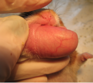
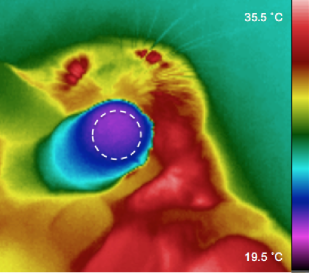
Figure 1(a) shows the normal hamster cheek pouch tissue. The measured temperature values during time were extracted from the thermal image (Figure 1(b)) and averaged in a user-defined region of interest (ROI) used to delineate the normal tissue.
5.2 Determination of the superficial temperature and superficial heat loss
In this study, the differential equation model (1) was applied to model the hamster cheek pouch temperature, imposing a loss of heat in the superficial tissue, due to the water evaporation. For this simulation, we used the experimental temperature data as a function of time in a given ROI [9].
The heat transfer modeling in organs has proposed numerous equations, studied by Pennes since 1948 [22, 23]. He suggested that the heat transfer rate between blood and tissue was proportional to the product of the volumetric perfusion rate and the difference between the arterial blood temperature and the local tissue temperature. Therefore the temperature of a tissue depends on the rate of blood perfusion, the metabolic activity and the heat conduction between the tissue and the environment. Taking into account the suggestion made by Pennes [23], Eq. (1a) of problem (1) takes the form:
| (14) |
where () represents the tissue (blood) density, () is the tissue (blood) specific heat, is the thermal conductivity, is the blood perfusion coefficient, is the metabolic heat source and is the constant blood temperature. The boundary condition Eqs. (1b), (1c) and (1d) are:
| (15) |
Where, represents the inner boundary and let represents the superficial boundary. Here, () represents the superficial heat loss due to water evaporation, is the heat transfer coefficient between the tissue and the air and is the ambient temperature. We used the following initial temperature, that assures the continuity of the temperature values between the two boundaries and :
| (16) |
where is the initial superficial temperature measured. We used a linear function for simplicity.
Since thermal responses in the hamster cheek pouch were assessed before, during and after the application of a thermal stimulus (TEP, PT and RP) [9], these three different phases were modeled considering that the heat transfer coefficient assumed different values in each stage:
| (17) |
The values used for and and others parameters are shown in Table 1.
| 28.715 | 28.5 | 35 | 10 | 30 | 10 |
To our knowledge, there are no published data related to the thermophysical properties (such as thermal conductivity, diusivity, etc.) of the hamster cheek pouch. In [24], Poppendiek et al. suggested that tissues may be considered accurately for thermal analysis as being composed of water, protein and fat. Thus, for the thermal properties needed to compute Eq. (10) in our biological application, we only considered water and protein to calculate the thermal properties, shown in Table 2. The other parameters not related to the composition of the tissue were obtained from [25].
| (W/m ∘C) | (W/m3 ∘C) | (Kg/m3) | (Kg/m3) | (J/Kg ∘C) | (J/Kg ∘C) | (W/m3) |
| 0.445 | 0.0002 | 1200 | 1060 | 3300 | 3770 | 368.1 |
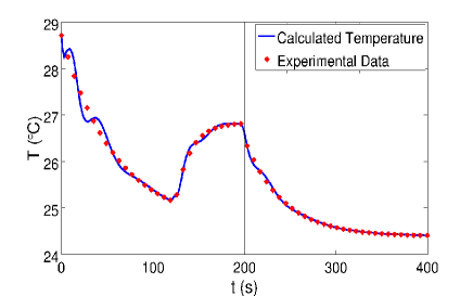
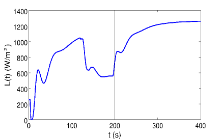
Figure 2 shows the normal hamster cheek pouch experimental and calculated thermal response as a function of time. In Figure 2(a) it can be seen the good approximation between the calculated superficial temperature and the experimental data. In particular, Figure 2(b) depicts the convective coefficient obtained using an initial constant coefficient , and 15 steps of the gradient descent method described in Section 3.
In Figure 2(b), we observed that at the beginning of each stage the superficial heat loss had oscillations. These oscillations can be seen also in the derivative of the functional (see Eq. (2)), and therefore it seems that they are intrinsic of this differential problem. Besides, during the provocation test, the superficial heat loss decreases, due to the air stimulus that helps to eliminate the tissue superficial moisture.
5.3 Sensitivity analysis
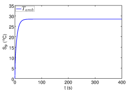
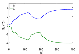
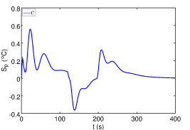
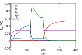
Table 1 and 2 show those parameters used for the sensitivity analysis. We also used the parameter in Figure 2(b), obtained in the previous section. The initial temperature is in Eq. (16). Table 3 summarizes the physiological parameters considered, showing their units, and their position in the differential problem444The position in the differential problem, which was taken into account when the sensitivity was computed, changing the parameter to whenever it appeared., necessary for the sensitivity analysis. Note that some parameters, such as and , appeared in more than one place in the differential problem. Figure 3 shows different parameters sensitivities, grouped together depending on their order of the sensitivity. A summary of the order of the sensitivity parameters is shown in Table 4.
| Symbol | Units | Represents | Position in the differential problem∗ |
|---|---|---|---|
| ∘C | temperature of tissue | DE, BC. | |
| 1/ | blood perfusion | DE: indep. term, heat source | |
| W/m ∘C | tissue conductivity | DE: second order term | |
| BC: external normal derivative | |||
| Kg/m3 | tissue density | DE: temporal derivative | |
| Kg/m3 | blood density | DE: temporal derivative | |
| J/Kg ∘C | specific heat of tissue | DE: temporal derivative | |
| J/Kg ∘C | specific heat of blood | DE: temporal derivative | |
| m2/ | diffusivity of tissue | DE: second order term | |
| 1/ | diffusivity of blood | DE: independent term | |
| W/m3 | metabolic heat | DE: heat source | |
| W/m3 | DE: heat source | ||
| ∘C | ambient temperature | BC: convective condition | |
| ∘C | arterial temperature | DE: heat source | |
| BC: Dirichlet condition | |||
| ∘C | inferior temperature | BC: Dirichlet condition | |
| ∘C | superficial temperature in | BC: Dirichlet condition | |
| ∘C | initial temperature | BC: Dirichlet condition | |
| W/m2 ∘C | tissue-air convective coeff. | BC: convective condition | |
| W/m2 | superficial heat loss | BC: convective condition | |
| m | tissue depth | EDP: Domain |
| Order of the sensitivity | Parameters |
|---|---|
| 10 | |
| 1 | |
The first important observation is that the most sensible parameter is the ambient temperature () (Figure 3(a)). This could be explained by the thinness of the tissue and the Dirichlet condition in the inner surface. Therefore, this parameter should be determined with the smallest error possible.
Secondly, we examined the linear dependence between parameters, studied in [26], which could be established by analyzing the shapes of the sensitivity parameters. If two parameters are linearly dependent, this means that there are infinite possible solutions, which implies that there will be infinite local minimums and therefore the minimization problem will not converge.
Figure 3(b) shows that and are linearly dependent parameters, because their sensitivity are symmetric with respect to the horizontal axis. Therefore, although they have similar sensitivities, they should not be simultaneously determined. Figure 3(d) shows that and are linearly dependent parameters, because their sensitivities have the same behavior (increasing functions). Moreover, these parameters are linearly dependent with and . Therefore to determine a parameter, of this order of sensitivity, we should choose between , and .
Finally the least sensible parameter is the metabolic heat , which may be justified by observing that the total heat source is , and the predominant term is .
6 Conclusions
We proposed a method for the determination of time dependent parameters using measured superficial temperatures in a conduction problem with evaporation, and a new way of computing a sensitivity analysis of a variable parameter. We applied this method successfully to a biological problem, modeling tissue temperature changes, under transient conditions, in the hamster cheek pouch. In this study we found a good approximation between the calculated superficial temperature and the experimental data. We performed a sensitivity analysis, which should be done whenever parameters are simultaneously determined. Based on temperature measurements and having calculated the loss of heat due to water evaporation at the superficial layer of the pouch, the sensitivity analysis determined which of the studied parameters were the most sensible to variations of the superficial experimental data. We found that ambient temperature should be measured with the smallest error, because it is the most sensible parameter in this problem. Moreover, we noted that the linear dependence between the conductivity and the superficial heat loss is not intuitive, in contrast with the dependence between the blood perfusion and the blood temperature (an increase in either of them would result in a raise in the superficial temperature). Therefore, we conclude that a choice has to be made between determining the conductivity or the superficial heat loss.
In previous studies, we observed that tumors and particularly a precancerous tissue bearing ulcers after BNCT had high superficial humidity [9]. Thus, in future studies, the proposed mathematical model will be extended to explore the mass moisture transfer as a function of time in tumors and precancerous tissue in the hamster cheek pouch.
Acknowledgments
This paper has been partially supported by the BNCT project of CNEA, and by CONICET.
References
- [1] S. G. Bankoff, “Heat conduction or diffusion with change of phase,” Advances in Chemical Engineering, vol. 5, pp. 75–150, 1964.
- [2] J. J. Roering, J. W. Kirchner, and W. E. Dietrich, “Evidence for nonlinear, diffusive sediment transport on hillslopes and implications for landscape morphology,” Water Resources Research, vol. 35 (3), pp. 853–870, 1999.
- [3] L. S. Andrew, “Wildland surface fire spread modelling, 1990–2007. 1: Physical and quasi-physical models,” International Journal of Wildland Fire, vol. 18, pp. 349–368, 2009.
- [4] R. Baini and T. A. G. Langrish, “Choosing an appropriate drying model for intermittent and continuous drying of bananas,” Journal of Food Engineering, vol. 79, pp. 330–343, 2007.
- [5] M. P. Tolaba, R. J. Aguerre, and C. Suárez, “Modeling cereal grain drying with variable diffusivity,” Cereal Chem, vol. 74, pp. 842–845, 2007.
- [6] C. Suárez and P. E. Viollaz, “Shrinkage effect on drying behavior of potato slabs,” Journal of Food Engineering, vol. 13, pp. 103–114, 1991.
- [7] M. Paruch and E. Majchrzak, “Identification of tumor region parameters using evolutionary algorithm and multiple resiprocity boundary element method,” Eng. Appl. Artificial Intelligence, vol. 20, pp. 647–655, 2007.
- [8] F. S. Bazán, L. Bedin, and L. S. Borges, “Space-dependent perfusion coefficient estimation in a 2d bioheat transfer problem,” Computer Physics Communications, vol. 214, pp. 18–30, 2017.
- [9] M. Herrera, A. Monti Hughes, N. Salva, C. Padra, A. Schwint, and G. A. Santa Cruz, “Non-invasive characterization of normal and pathological tissues through dynamic infrared imaging in the hamster cheek pouch oral cancer model,” SPIE Proceedings: Thermosense: Thermal Infrared Applications XXXIX Paolo Bison; Douglas Burleigh, Editor(s), vol. 10214, 2017.
- [10] O. Pironneau, Optimal Shape Design for Elliptic Systems. Springer-Verlag, New York, 1984.
- [11] B. F. Blackwell and K. J. Dowding, Handbook of Numerical Heat Transfer, Chapter 14: Sensitivity analysis ans uncertainty propagation of computational models. Kluwer Academic, Netherlands, 1989.
- [12] K. Benke, K. Lowell, and A. Hamilton, “Parameter uncertainty, sensitivity analysis and prediction error in a water-balance hydrological model,” Mathematical and Computer Modelling, vol. 47, pp. 1134–1149, 2008.
- [13] G. A. Santa Cruz, S. J. González, A. Dagrosa, A. E. Schwint, M. Carpano, V. A. Trivillin, E. F. Boggio, J. Bertotti, J. Marín, A. Monti Hughes , A. J. Molinari, and M. Albero, “Dynamic infrared imaging for biological and medical applications in boron neutron capture therapy,” in Thermosense: Thermal Infrared Appl. XXXIII (M. Safai and J. R. Brown, eds.), vol. 8013, (Orlando, Florida, USA), pp. 7–25, SPIE, 2011.
- [14] A. Monti Hughes, R. F. Aromando, M. A. P. andA. E. Schwint, and M. E. Itoiz, “The hamster cheek pouch model for field cancerization studies,” Periodontol 2000, vol. 67, pp. 292–311, 2015.
- [15] J. A. Coderre and G. M. Morris, “The radiation biology of boron neutron capture therapy,” Radiat Res., vol. 151(1), pp. 1–18, 1999.
- [16] D. L. Kellogg, “In vivo mechanisms of cutaneous vasodilation and vasoconstriction in humans during thermoregulatory challenges,” J. Appl. Physiol., vol. 100(5), pp. 1709–1718, 2006.
- [17] G. A. Santa Cruz, S. J. González, J. Bertotti, and J. Marín, “First application of dynamic infrared imaging in boron neutron capture therapy for cutaneous malignant melanoma,” Med. Phys., vol. 36, pp. 4519–4529, 2009.
- [18] N. Arora, D. M. andD. Ruggerio, E. Tousimis, A. J. Swistel, M. P. Osborne, and R. M. Simmons, “Effectiveness of a noninvasive digital infrared thermal imaging system in the detection of breast cancer,” The American Journal of Surgery, vol. 196, pp. 523–526, 2008.
- [19] C. Hildebrandt, C. Raschner, and K. Ammer, “An overview of recent application of medical infrared thermography in sports medicine in austria,” Sensors, vol. 10, pp. 4700–4715, 2010.
- [20] M. P. Çetingül and C. Herman, “Quantification of the thermal signature of a melanoma lesion,” Clinics in Dermatology, vol. 13, pp. 329–336, 2011.
- [21] G. Bhavani Bharathi, S. V. Francis, M. Sasikala, Sandeep, and D. Jaipurka, “Feature analysis for abnormality detection in breast thermogram sequences subject to cold stress,” in Proceedings of The National Conference on Man Machine Interaction 2014 (M. H. Loew, ed.), NCMMI 2014, pp. 15–21, 2014.
- [22] H. W. Huang, C. L. Chan, and R. B. Roemer, “Analytical solutions of pennes bio-heat transfer equation with blood vessel,” J. of Biomechanical Engineering, vol. 116, pp. 208–212, 1994.
- [23] H. Pennes, “Analysis of tissue ans arterial blood temperature in the resting human forearm,” J. Appl. Physiol., vol. 1, pp. 93–122, 1948.
- [24] H. F. Poppendiek, R. Randall, J. Breeden, J. E. Chambers, and J. R. Murphy, “Thermal conductivity measurements and predictions for biological fluids and tissues,” Cryobiology, vol. 3, pp. 318–327, 1966.
- [25] M. Pirtini Cetingul and C. Herman, “A heat transfer model of skin tissue for the detection of lesions: sensitivity analysis,” Phys. Med. Biol., vol. 55, pp. 5933–5951, 2010.
- [26] J. Beck and K. Arnold, Parameter estimation in engineering and sciences. John Wiley & Sons, 1977.