Efficient Deformable Shape Correspondence via Kernel Matching

Abstract

We present a method to match three dimensional shapes under non-isometric deformations, topology changes and partiality. We formulate the problem as matching between a set of pair-wise and point-wise descriptors, imposing a continuity prior on the mapping, and propose a projected descent optimization procedure inspired by difference of convex functions (DC) programming.

1 Introduction

Finding correspondences between non-rigid shapes is a fundamental problem in computer vision, graphics and pattern recognition, with applications including shape comparison, texture transfer, and shape interpolation just to name a few. Given two three-dimensional objects $\mathcal{X}$ and $\mathcal{Y}$, modeled as compact two-dimensional Riemannian manifolds, our task is to find a meaningful correspondence $\varphi:\mathcal{X}\rightarrow\mathcal{Y}$. While a rigorous definition of meaningful is challenging, one can identify some desirable properties of $\varphi$:

1. Bijective.

2. Continuous in both directions, in the sense that nearby points on $\mathcal{X}$ should be mapped to nearby points on $\mathcal{Y}$ (and vice versa).

3. Similar points should be put into correspondence.

For the simplicity of the introduction, we assume the two shapes $\mathcal{X}$ and $\mathcal{Y}$ to be sampled at $n$ points each, and defer the case of different number of samples to the algorithmic part of this paper detailed in Section 3. Assuming a consistent sampling (e.g. via farthest point sampling with a sufficiently large number $n$ of points), the discrete counterpart to the correspondence $\varphi$ is a mapping $\pi:\{x_{1},\ldots x_{n}\}\rightarrow\{y_{1},\ldots y_{n}\}$, which admits a representation as a permutation matrix $\mathbf{\Pi}\in\{0,1\}^{n\times n}$ satisfying $\mathbf{\Pi}^{\top}\mathbf{1}=\mathbf{\Pi}\mathbf{1}=\mathbf{1}$ with $\mathbf{1}$ being a column vector of ones. We henceforth denote the space of $n\times n$ permutation matrices by $\mathcal{P}_{n}$.

The vast majority of shape matching approaches phrase the correspondence problem as an energy minimization problem

$${\mathbf{\Pi}}^{*} =\arg\!\!\min_{\mathbf{\Pi}\in\mathcal{P}_{n}}E({\mathbf{\Pi}})\,,$$ (1)

where $E(\mathbf{\Pi})$ is usually a weighed aggregate of two terms

$$E(\mathbf{\Pi})=\alpha g(\mathbf{\Pi})+h(\mathbf{\Pi})\,.$$ (2)

The first term $g(\mathbf{\Pi})$ is a fidelity term trying to align a set of pointwise descriptors encoding the similarity between points, while the second term $h(\mathbf{\Pi})$ is a regularization term promoting the continuity of the correspondence by aligning a set of pairwise descriptors encoding global/local relations between pairs of points. The parameter $\alpha$ governs the tradeoff between the two terms.

While the constraint $\mathbf{\Pi}\in\mathcal{P}_{n}$ guarantees bijectivity of the correspondence, the two terms $h$ and $g$ correspond, respectively, to the second and the third desirable qualities of a meaningful correspondence, and provide a trade-off between complexity, fidelity and regularity. We stress in our work that despite their seemingly unrelated nature, those properties are in fact tightly connected, i.e., choosing a particular set of pairwise descriptors might have a profound effect not only on the regularity of the final solution, but also on the complexity of the resulting optimization problem. We will elaborate on these aspects in more detail.

Related work. Finding correspondences between shapes is a well-studied problem. Traditionally, the solution involves minimization of a distortion criterion which fits into one of the two categories: pointwise descriptor similarity [43, 49, 16, 4, 51], and pairwise relations [34, 17, 18, 52]. In the former case, matches are obtained via nearest neighbor search or, when injectivity is required, by solving a linear assignment problem (LAP). Pairwise methods usually come at a high computational cost, with the most classical formulation taking the form of an NP-hard quadratic assignment problem (QAP) [37]. Several heuristics have been proposed to address this issue by using subsampling [50] or coarse-to-fine techniques [54, 44]. Various relaxations have been used to make the QAP problem tractable [13, 27, 39, 1, 17, 21], however they result in approximate solutions. In addition, pairwise geodesics are computationally expensive, and sensitive to noise. In [20] the use of heat kernels was proposed as a noise-tolerant approximation of matching adjacency matrices. In [53] dense bijective correspondences were derived from sparse and possibly noisy input using an iterative filtering scheme, making use of geodesic Gaussian kernels.

A different family of methods look for pointwise matches in a lower-dimensional “canonical” embedding space. Such embedding can be carried out by multidimensional scaling [19, 12] or via the eigenfunctions of the Laplace-Beltrami operator (LBO) [33, 48]. The correspondence is then calculated in the embedding space using a simple rigid alignment technique such as ICP [6]. Functional maps [36, 23] can be seen as a sophisticated way to initialize ICP when using this spectral embedding. Other bases can be used within the functional map framework [24]. In particular, the eigenspaces arising from the spectral decomposition of the geodesic distance matrices have been shown to outperform the LBO basis for the case of isometric shapes [46]. In [55] the matching problem is phrased as an integer linear program, enforcing continuity of the correspondence via a linear constraint. This additional constraint however makes the problem computationally intractable even for modestly-sized shapes, requiring the use of relaxation and post-processing heuristics.

Most recent works attempt to formulate the correspondence problem as a learning problem [42] and design intrinsic deep learning architectures on manifolds and point clouds [32, 9, 11, 10, 35, 29]. As of today, these methods hold the record of performance on deformable correspondence benchmarks; however, supervised learning requires a significant annotated training set that is often hard to obtain.

Contribution. The main contribution of this paper is a simple method that works out-of-the-box for finding high quality continuous (regular) correspondence between two not necessarily isometric shapes. The method can be seen as an improved version of [53], and is accompanied by theoretical insights that shed light on its effectiveness. In particular, we contrast the method with other shape matching approaches and elaborate on the computational benefits of using kernels rather than distances as pairwise descriptors. The key insight is the realization that high quality regular correspondence can be obtained from a rough irregular one by a sequence of smoothing and projection operations. Remarkably, this process admits an appealing interpretation as an alternating diffusion process [26]. We report drastic runtime and scalability improvements compared to [53], and present an extension to the setting of partial shape correspondence and an effective multi-scale approach.

2 Background

2.1 Pointwise descriptors

Similarity of points is often measured with the help of pointwise descriptors $f_{\mathcal{X}}:\mathcal{X}\rightarrow\mathbb{R}^{q}$, $f_{\mathcal{Y}}:\mathcal{Y}\rightarrow\mathbb{R}^{q}$ that are constructed in a way such that similar points on the two shapes are assigned closeby (in the Euclidean sense) descriptors, while dissimilar points are assigned distant descriptors. In the discrete case, the descriptors $f_{\mathcal{X}},f_{\mathcal{Y}}$ can be encoded as matrices $\mathbf{F}_{\mathcal{X}},\mathbf{F}_{\mathcal{Y}}\in\mathbb{R}^{n\times q}$ giving rise to the optimization problem

$$\arg\!\!\min_{\mathbf{\Pi}\in\mathcal{P}_{n}}\left\|{\mathbf{\Pi}}\mathbf{F}_{\mathcal{X}}-\mathbf{F}_{\mathcal{Y}}\right\|^{2}=\arg\!\!\max_{\mathbf{\Pi}\in\mathcal{P}_{n}}\langle{\mathbf{\Pi}},\mathbf{F}_{\mathcal{Y}}\mathbf{F}_{\mathcal{X}}^{\top}\rangle\,.$$ (3)

Problem (3) is linear in ${\mathbf{\Pi}}$ and is therefore one of the rare examples of combinatorial optimization problems that can be globally optimized in polynomial time; the best known complexity $O(n^{2}\log n)$ is achieved by the auction algorithm [5].

Over the last years, intrinsic features have extensively been used due to their invariance to isometry. However, they come with two main drawbacks: First, the implicit assumption that the shapes at hand are isometric is not always met in practice. Today’s best performing approaches partially tackle this problem using deep learning [32, 9, 11, 10, 35]. Secondly, many natural shapes come with at least one intrinsic (e.g., bilateral) symmetry that is impossible to capture by purely intrinsic features, be these handcrafted or learned. Correspondences obtained by (3) may suffer from severe discontinuities due to some points being mapped to the desired destination, and others to the symmetric counterpart.

2.2 Pairwise descriptors

Another family of methods consider pairwise descriptors of the form $d_{\mathcal{X}}:\mathcal{X}\times\mathcal{X}\rightarrow\mathbb{R}$, $d_{\mathcal{Y}}:\mathcal{Y}\times\mathcal{Y}\rightarrow\mathbb{R}$ encoded in the discrete setting as symmetric matrices $\mathbf{D}_{\mathcal{X}},\mathbf{D}_{\mathcal{Y}}\in\mathbb{R}^{n\times n}$. These methods aim at solving optimization problems of the form

$${\mathbf{\Pi}}^{*} =\arg\!\!\min_{\mathbf{\Pi}\in\mathcal{P}_{n}}\left\|{\mathbf{\Pi}}\mathbf{D}_{\mathcal{X}}-\mathbf{D}_{\mathcal{Y}}{\mathbf{\Pi}}\right\|^{2}$$ (4)

$$=\arg\!\!\max_{\mathbf{\Pi}\in\mathcal{P}_{n}}\langle{\mathbf{\Pi}},\mathbf{D}_{\mathcal{Y}}{\mathbf{\Pi}}\mathbf{D}_{\mathcal{X}}\rangle\,,$$ (5)

known under the names of graph matching (GM) or quadratic assignment problem (QAP), and are in general not solvable in polynomial time. A typical way to circumvent the complexity issue is to relax the integer constraint $\pi_{ij}\in\{0,1\}$ and optimize the objectives (4)-(5) over the convex set of bi-stochastic matrices $\mathcal{B}_{n}=\{{\mathbf{P}}\geq\mathbf{0}:{\mathbf{P}}^{\top}\mathbf{1}={\mathbf{P}}\mathbf{1}=\mathbf{1}\}$. Note that when viewed as functions over this convex set, the objectives (4)-(5) are no longer equivalent. In particular, (4) will always be convex, while the convexity of (5) depends on the eigenvalues of the matrices $\mathbf{D}_{\mathcal{X}}$ and $\mathbf{D}_{\mathcal{Y}}$, as shown in the following lemma.

Lemma 1.

Let $\mathbf{D}_{\mathcal{X}},\mathbf{D}_{\mathcal{Y}}$ be symmetric. The function $h(\mathbf{P})=\langle{\mathbf{P}},\mathbf{D}_{\mathcal{Y}}{\mathbf{P}}\mathbf{D}_{\mathcal{X}}\rangle$ over the set of bi-stochastic matrices $\mathcal{B}_{n}$ is (strictly) convex iff all eigenvalues of $\mathbf{D}_{\mathcal{X}}$ and $\mathbf{D}_{\mathcal{Y}}$ are (strictly) positive.

Corollary 1.

If all eigenvalues of $\mathbf{D}_{\mathcal{X}}$ and $\mathbf{D}_{\mathcal{Y}}$ are strictly positive, the optimum of the relaxed problem coincides with that of the original combinatorial problem:

$$\arg\!\!\max_{\mathbf{P}\in\mathcal{B}_{n}}h(\mathbf{P}) =\arg\!\!\max_{\mathbf{\Pi}\in\mathcal{P}_{n}}h(\mathbf{\Pi})\,.$$ (6)

Notice that we can add a linear term (weighted by a scalar factor $\alpha$), such as the one in (3), while still keeping this property: $E(\mathbf{P})=\alpha\langle{\mathbf{P}},\mathbf{F}_{\mathcal{Y}}\mathbf{F}_{\mathcal{X}}^{\top}\rangle+\langle{\mathbf{P}},\mathbf{D}_{\mathcal{Y}}{\mathbf{P}}\mathbf{D}_{\mathcal{X}}\rangle\,$.

Figure 2: Spectrum of distance matrix (left) vs. spectrum of heat-kernel matrix (right) for several values of $t\in[0.01,5]$ computed on the cat shape from TOSCA.

Popular pairwise descriptors include a variety of pairwise distances [13, 15, 38] and kernels [31, 47, 53] tailored for the specific class of deformations. In what follows, we advocate the superiority of using kernels over distances.

Pairwise distances. A common choice for pairwise descriptors are geodesic distances $d_{\mathcal{X}}(x_{i},x_{j})$, a choice motivated by the fact that, for isometric shapes, these are preserved by the optimal ${\mathbf{\Pi}}$. Geodesic distances have major drawbacks, both from the modeling and computational point of view. On the modeling side, they introduce a bias towards far away points and are sensitive to topological noise. On the computational side, they are slow to compute and give rise to highly non-convex (and non-differentiable) optimization problems. Note that, although one may employ more robust definitions of distance [15, 17], these do not solve the optimization issues.

Heat kernels. Heat kernels are fundamental solutions to the heat diffusion equation on manifold $\mathcal{X}$,

$$\frac{\partial u(t,x)}{\partial t} =\Delta_{\mathcal{X}}u(t,x)\,,$$ (7)

with the initial condition $u(0,x)=u_{0}(x)$ and additional boundary conditions if applicable. Here $u:[0,\infty)\times\mathcal{X}\rightarrow\mathbb{R}$ represents the amount of heat at point $x$ at time $t$. The solution is linear in the initial distribution and is given by

$$u(t,x) =\int_{\mathcal{X}}k(t,x,x^{\prime})u_{0}(x^{\prime})dx^{\prime}\,,$$ (8)

where $k:\mathbb{R}^{+}\times\mathcal{X}\times\mathcal{X}\rightarrow\mathbb{R}$ is the heat kernel and its values can be interpreted as the amount of heat transported from $x^{\prime}$ to $x$ in time $t$. In the Euclidean case, the heat kernel is an isotropic Gaussian kernel with the variance proportional to the diffusion time $t$.

Figure 3: Runtime comparison of matching shapes with varying number of vertices using our algorithm with heat kernels compared to Gaussian kernels[53]. For more info see supp. material.

For a compact manifold $\mathcal{X}$, the heat kernel can be expressed as the exponent of the intrinsic self-adjoint negative semi-definite Laplacian operator $\Delta_{\mathcal{X}}$,

$$k(t,x,x^{\prime}) =\sum_{i}e^{\lambda_{i}t}\phi_{i}(x)\phi_{i}(x^{\prime}),$$ (9)

where $\Delta_{\mathcal{X}}\phi_{i}(x)=\lambda_{i}\phi_{i}(x)$ is the eigendecomposition of the Laplacian with eigenvectors $\phi_{1},\phi_{2},\ldots$ and corresponding non-positive eigenvalues $0=\lambda_{1}\geq\lambda_{2}\geq\ldots$. The null eigenvalue is associated with a constant eigenvector.

In the discrete setting, the heat kernel is given by the positive-definite matrix $\mathbf{K}_{\mathcal{X}}=e^{t\boldsymbol{\Delta}_{\mathcal{X}}}=\boldsymbol{\Phi}e^{t\boldsymbol{\Lambda}_{\mathcal{X}}}\boldsymbol{\Phi}^{\top}$. The constant eigenvector corresponds to the unit eigenvalue, $\mathbf{K}_{\mathcal{X}}\mathbf{1}=\mathbf{1}$.

An issue that is often overlooked is the relation between the original and relaxed solution of (5), which is tightly connected to the choice of pairwise descriptors. Corollary 1 asserts the sufficient condition under which this relaxation is exact. Whereas heat kernels, being (strictly) positive definite, satisfy this condition, distance matrices never do. A distance matrix, having non-negative entries and trace zero, will always, by the Perron-Frobenius theorem, have one large positive eigenvalue and several low magnitude negative eigenvalues [8]. This distribution of eigenvalues is illustrated in Figure 2.

2.3 Bijective maps and functional maps

The requirement of bijectivity is what makes a problem (1) computationally hard. A variety of relaxation techniques can be applied to alleviate this complexity. Amongst the most popular are relaxing the column or row sum constraints, relaxing the integer constraints, or restricting the matrix to a sphere of constant norm [27]. A bijective mapping can then be recovered by a post processing step, such as projection onto the set of permutation matrices

$$\mathbf{\Pi}^{*}=\arg\!\!\min_{\mathbf{\Pi}\in\mathcal{P}_{n}}\|\mathbf{\Pi}-\mathbf{P}\|^{2}=\arg\!\!\max_{\mathbf{\Pi}\in\mathcal{P}_{n}}\left<\mathbf{\Pi},\mathbf{P}\right>\,.$$ (10)

One popular technique in recent years replaces the combinatorially hard point-wise map recovery problem with the simpler problem of finding a linear map between functions[36]. A functional map is a map between functional spaces $T:L^{2}(\mathcal{X})\rightarrow L^{2}(\mathcal{Y})$, which can be disretized (under the previous assumptions of $n$ vertices in each shape) as an $n\times n$ matrix $\mathbf{T}$. Providing a pair of orthonormal bases $\boldsymbol{\Phi}=(\boldsymbol{\phi}_{1},\ldots,\boldsymbol{\phi}_{n})$ and $\boldsymbol{\Psi}=(\boldsymbol{\psi}_{1},\ldots,\boldsymbol{\psi}_{n})$ for $L^{2}(\mathcal{X})$ and $L^{2}(\mathcal{Y})$, respectively, one can express $\mathbf{T}=\boldsymbol{\Psi}\mathbf{C}\boldsymbol{\Phi}^{\top}$, where $\mathbf{C}$ acts as a basis transformation matrix. Two common choices for basis are the Dirac (or hat) basis, in which the functional map attains the form of a permutation matrix, and the Laplacian eigenbasis, which is especially suited when the map is smooth, so it can be approximated using a truncated basis of $k$ first basis functions corresponding to the lowest frequencies. The computation of the functional map thus boils down to solving a linear system $\mathbf{C}\boldsymbol{\Phi}^{\top}\mathbf{F}_{\mathcal{X}}=\boldsymbol{\Psi}^{\top}\mathbf{F}_{\mathcal{Y}}$. The recovery of the point-wise map from the functional map can be obtained by ICP-like procedures [36, 41], with the possible introduction of bijectivity constraints [53]. The fact that the map is band-limited is often erroneously referred to as “smoothness” in the literature; however, the bijective map recovered from such a band-limited map is not guaranteed to be continuous let alone smooth (i.e., continuously differentiable).

3 Method

3.1 Optimization

We aim at maximizing $E(\mathbf{\Pi})$ over $\mathcal{P}_{n}$, which by Corollary 1 is equivalent to the relaxed problem

$$\arg\!\!\max_{\mathbf{P}\in\mathcal{B}_{n}}E(\mathbf{P})=\arg\!\!\max_{\mathbf{P}\in\mathcal{B}_{n}}\langle{\mathbf{P}},\alpha\mathbf{F}_{\mathcal{Y}}\mathbf{F}_{\mathcal{X}}^{\top}+\mathbf{K}_{\mathcal{Y}}{\mathbf{P}}\mathbf{K}_{\mathcal{X}}\rangle$$ (11)

where $\mathbf{F}_{\mathcal{X}},\mathbf{F}_{\mathcal{Y}}$ are matrices of pointwise descriptors and $\mathbf{K}_{\mathcal{X}},\mathbf{K}_{\mathcal{Y}}$ are the positive-definite heat kernel matrices on $\mathcal{X}$ and $\mathcal{Y}$, respectively. This maximization problem can be seen as the minimization of the difference of convex functions:

$$\arg\!\!\min_{\mathbf{P}\in\mathbb{R}^{n\times n}}B(\mathbf{P})-E(\mathbf{P}).$$ (12)

where $B$ is the (convex) indicator function on the set of bistochastic matrices $\mathcal{B}_{n}$.

A renowned way to optimize this type of energy is the difference of convex functions (DC) algorithm that starts with some initial $\mathbf{P}^{0}$ and then iterates the following two steps until convergence:

• Select $\mathbf{Q}^{k}\in\partial E(\mathbf{P}^{k})$.

• Select $\mathbf{P}^{k+1}\in\partial B^{*}(\mathbf{Q}^{k})$.

Here $B^{*}$ denotes the convex conjugate of $B$ and $\partial E,\partial B^{*}$ denote the subdifferentials (set of supporting hyperplanes) of $E$ and $B^{*}$, respectively.

For a differentiable $E$, the step of the DC algorithm assumes the form

$$\mathbf{P}^{k+1}=\arg\!\!\max_{\mathbf{P}\in\mathcal{B}_{n}}\langle\mathbf{P},\nabla E(\mathbf{P}^{k})\rangle\,.$$ (13)

Moreover, the value of the objective is an increasing sequence, $E(\mathbf{P}^{k+1})>E(\mathbf{P}^{k})$, and each iterate $\mathbf{P}^{k}$ is a permutation matrix. We provide the proof in the supplementary material. Figure 4 illustrates this iterative process.

Since $\mathbf{P}^{k}$ is guaranteed to be a permutation matrix, we henceforth use $\mathbf{\Pi}^{k}$ to denote the iterates. For our choice of $E$, the gradient is given by

$$\nabla E =\alpha\mathbf{F}_{\mathcal{Y}}\mathbf{F}_{\mathcal{X}}^{\top}+\mathbf{K}_{\mathcal{Y}}{\mathbf{\Pi}}\mathbf{K}_{\mathcal{X}}$$ (14)

yielding the step

$$\mathbf{\Pi}^{k+1} =\arg\!\!\max_{\mathbf{\Pi}\in\mathcal{B}_{n}}\langle\mathbf{\Pi},\alpha\mathbf{F}_{\mathcal{Y}}\mathbf{F}_{\mathcal{X}}^{\top}+\mathbf{K}_{\mathcal{Y}}{\mathbf{\Pi}}^{k}\mathbf{K}_{\mathcal{X}}\rangle\,.$$ (15)

In the experiments presented in this paper, we use the data fidelity term $\langle\mathbf{\Pi},\mathbf{F}_{\mathcal{Y}}\mathbf{F}_{\mathcal{X}}^{\top}\rangle$ mainly to initialize the process:

$$\mathbf{\Pi}^{0} =\arg\!\!\max_{\mathbf{\Pi}\in\mathcal{B}_{n}}\langle\mathbf{\Pi},\mathbf{F}_{\mathcal{Y}}\mathbf{F}_{\mathcal{X}}^{\top}\rangle.$$ (16)

Figure 4: Schematic illustration of the proposed algorithm for maximizing a convex quadratic objective over a convex polytope, by successively maximizing a linear sub-estimate of it. The hot color map encodes the function values. The jet color map encodes the values of the linear sub-estimate. The point around which the objective is linearized is depicted in red. The global maximum is depicted in blue. The maximum of the linear sub-estimate is depicted in green. Notice that the algorithm travels between extreme but not necessarily adjacent points of the polytope, until it converges to a local maximum.

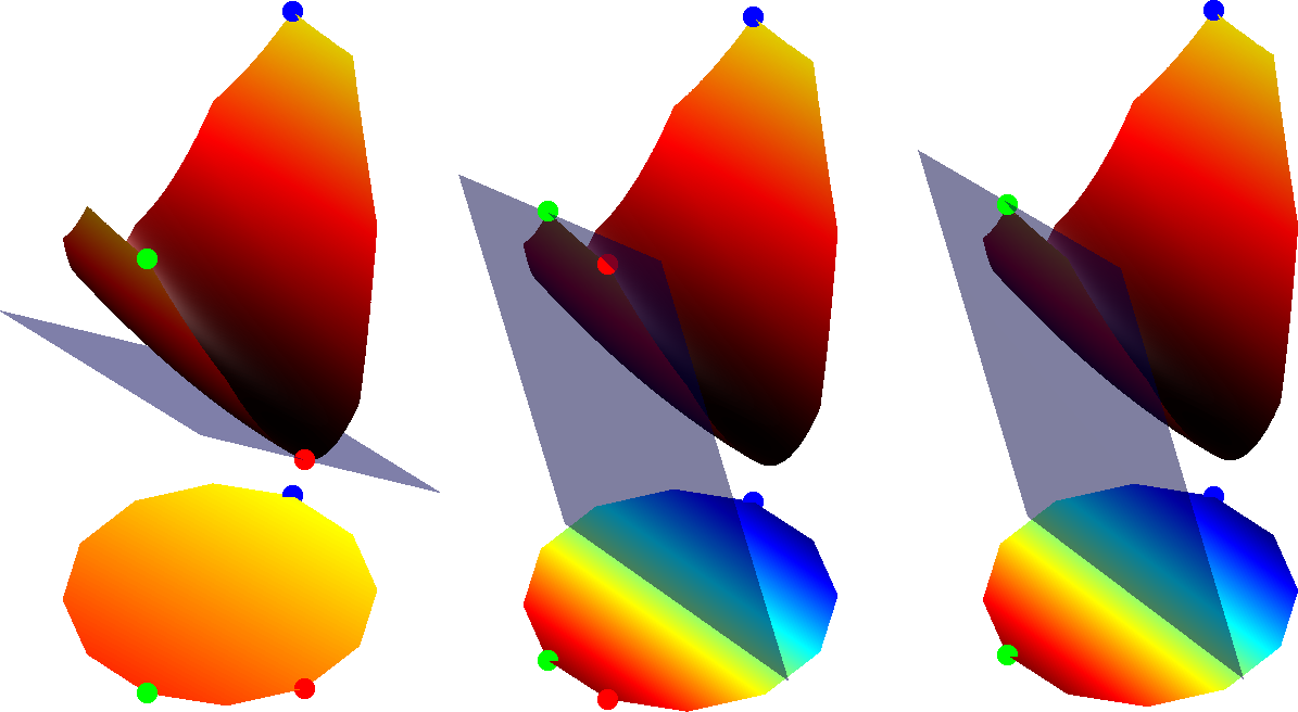
3.2 Partial matching using slack variables

\begin{overpic}[width=433.62pt]{figures/partiality.png} \put(8.0,0.0){Input} \put(34.0,0.0){Iter 1} \put(60.0,0.0){Iter 2} \put(87.0,0.0){Iter 3} \end{overpic}

Figure 5: Our approach can tackle the challenging scenario of partial correspondences. As a proof of concept we initialized our method with sparse correspondences, indicated by spheres. We simulated noise by mapping a point on the left hand of the woman to the right foot of the man. At the first iteration all points spread their information, leading to a discontinuity of the mapping at the hand of the woman. After three iterations the method converged to the correct solution. This example was generated with Gaussian kernels. The proper choice of boundary conditions when using heat kernels will be discussed in future work.

In a general setting, we will be dealing with shapes having different number of vertices. Let us denote by $n_{\mathcal{X}}$ the number of vertices on $\mathcal{X}$ and by $n_{\mathcal{Y}}$ the number of vertices on $\mathcal{Y}$, and assume w.l.o.g. $n_{\mathcal{X}}\geq n_{\mathcal{Y}}$. We aim at optimizing

$$\arg\!\!\max_{\mathbf{\Pi}\in\mathcal{P}_{n_{\mathcal{X}}}^{n_{\mathcal{Y}}}}\langle{\mathbf{\Pi}},\alpha\mathbf{F}_{\mathcal{Y}}\mathbf{F}_{\mathcal{X}}^{\top}+\mathbf{K}_{\mathcal{Y}}{\mathbf{\Pi}}\mathbf{K}_{\mathcal{X}}\rangle$$ (17)

where the space of rectangular permutation matrices $\mathcal{P}_{n_{\mathcal{X}}}^{n_{\mathcal{Y}}}$ is given by $\mathcal{P}_{n_{\mathcal{X}}}^{n_{\mathcal{Y}}}=\{\mathbf{\Pi}\in\{0,1\}^{n_{\mathcal{Y}}\times n_{\mathcal{X}}}:\mathbf{\Pi}\mathbf{1}\leq\mathbf{1},\mathbf{\Pi}^{\top}\mathbf{1}=\mathbf{1}\}$. Analogously to the previously discussed case in which we had $n_{\mathcal{X}}=n_{\mathcal{Y}}=n$, we iteratively solve

$$\mathbf{\Pi}^{k+1} =\arg\!\!\max_{\mathbf{\Pi}\in\mathcal{P}_{n_{\mathcal{X}}}^{n_{\mathcal{Y}}}}\langle\mathbf{\Pi},\alpha\mathbf{F}_{\mathcal{Y}}\mathbf{F}_{\mathcal{X}}^{\top}+\mathbf{K}_{\mathcal{Y}}{\mathbf{\Pi}^{k}}\mathbf{K}_{\mathcal{X}}\rangle\,.$$ (18)

In order to solve these optimization problems we pad the rectangular matrix $\alpha\mathbf{F}_{\mathcal{Y}}\mathbf{F}_{\mathcal{X}}^{\top}+\mathbf{K}_{\mathcal{Y}}{\mathbf{\Pi}^{k}}\mathbf{K}_{\mathcal{X}}$ with constant values $c$ (slack variables) such that it becomes square. After the correspondence is computed, we discard the ones belonging to the introduced slack variables. While such a treatment does not affect the value of the maximum, the constant $c$ has to be chosen appropriately to avoid ambiguity between the slacks and the actual vertices on $\mathcal{X}$. A drawback of this approach is that there are $(n_{\mathcal{X}}-n_{\mathcal{Y}})!$ solutions achieving the optimal score, leading to worse runtime in the presence of many slacks. See Fig.5. for a proof of concept of this approach.

3.3 Multiscale acceleration

Solving the LAP (18) at each iteration of the DC algorithm has a super-quadratic complexity. As a consequence, the proposed method is only directly applicable for small $n$ (up to $15\times 10^{3}$ in our experiments). We therefore propose a multiscale approach that enables us to find correspondences between larger meshes.

We start by resampling both shapes to a number of vertices we can handle and solving for a bijection $\pi_{0}:\mathcal{X}_{0}\to\mathcal{Y}_{0}$. This set of initial vertices is called seeds. The seeds on $\mathcal{X}$ are clustered into $k$ Voronoi cells and these cells are transfered to $\mathcal{Y}$ via $\pi_{0}$. More points are added iteratively and assigned to the same Voronoi cell as their closest seed. Next, we solve for $\pi_{i}:\mathcal{X}_{i}\to\mathcal{Y}_{i}$ where $i$ refers to the $i$-th Voronoi cell. This proceeds until all points are sampled (see Figure 6 for a visualization). To keep the correspondence consistent at the boundary of the Voronoi cells, we choose $1000$ correspondences from $\pi_{0}$ and use them to orient each Voronoi cell correctly over all iterations. Additional details are provided in the supplementary material.

\begin{overpic}[trim=0.0pt 0.0pt 0.0pt 0.0pt,clip,width=208.13574pt]{figures/multiscale1.png} \put(45.0,80.0){\footnotesize(a)} \end{overpic}

\begin{overpic}[trim=0.0pt 0.0pt 0.0pt 0.0pt,clip,width=208.13574pt]{figures/multiscale2.png} \put(45.0,80.0){\footnotesize(b)} \end{overpic}

\begin{overpic}[trim=0.0pt 0.0pt 0.0pt 0.0pt,clip,width=208.13574pt]{figures/multiscale3.png} \put(45.0,80.0){\footnotesize(c)} \end{overpic}

\begin{overpic}[trim=0.0pt 0.0pt 0.0pt 0.0pt,clip,width=208.13574pt]{figures/multiscale4.png} \put(45.0,80.0){\footnotesize(d)} \end{overpic}

Figure 6: Conceptual illustration of our multiscale approach: (a) correspondence at a coarse scale is given; (b) vertices on the source shape are grouped into sets (left), and the known correspondence is used to group vertices on the target shape (right); (c) vertices at a finer scale are added and (d) included in the group they reside in; finally, a correspondence is calculated for each group separately.

4 Interpretation

In what follows we provide different, yet complementary interpretations of the proposed method, shedding light on its effectiveness.

4.1 Alternating diffusion

To intuitively understand the efficacy of kernel alignment for the purpose of finding correspondences, consider the $k$-th iteration (without data term):

$$\max_{\mathbf{\Pi}\in\mathcal{P}_{n}}\langle\mathbf{\Pi},{K}_{\mathcal{Y}}\mathbf{\Pi}^{k}{K}_{\mathcal{X}}\rangle\,$$

Let us denote by $\boldsymbol{\delta}^{j}$ the discrete indicator function of vertex $j$ on shape $\mathcal{X}$, representing initial heat distribution concentrated at vertex $j$. This heat is propagated via the application of the heat kernel ${K}_{\mathcal{X}}$ to the rest of the vertices, resulting in the new heat distribution on $\mathcal{X}$ given by ${k}_{\mathcal{X}}^{j}={K}_{\mathcal{X}}{\boldsymbol{\delta}}^{j}$. This heat distribution, whose spread depends on the time parameter $t$, is mapped via $\mathbf{\Pi}^{k}$ onto the shape $\mathcal{Y}$, where it is propagated via the heat kernel ${K}_{\mathcal{Y}}$. The $ij$-th element of the matrix ${K}_{\mathcal{Y}}\mathbf{\Pi}^{k}{K}_{\mathcal{X}}$, Figure 7: Illustration of the alternating diffusion process initialized with a noisy correspondence that wrongly maps $\pi(8)=16$ and $\pi(16)=8$ but correctly maps $\pi(x)=x$ elsewhere. Top left: Indicator functions on the source shape, one on a point with a wrong correspondence (red) and one with a correct correspondence (blue). Top right: Both indicator functions are diffused. Bottom left: The diffused functions are transported to the target shape via $\pi$.Bottom right: Diffusion on the target shape.

4.2 Iterated blurring and sharpening

An alternative point of view is to recall that a diffusion process corresponds to a smoothing operation, or low-pass filtering in the spectral domain. To that end we view each iteration (15) as an application of a series of low-pass filters (smoothing) followed by a projection operation (deblurring/sharpening). To see that, we use the spectral decomposition of the heat kernels to rewrite the payoff matrix in (15)

where the functional map $\mathbf{C}$ is seen as a low-pass approximation of the permutation matrix in the truncated Laplacian eigenbasis, $\boldsymbol{\Pi}\approx{\Psi}\mathbf{C}{\Phi}^{\top}$. Equation (4.2) can thus be interpreted as applying a low-pass filter to the functional map matrix ${C}$. The second step in (15) can be regarded as a projection of the smoothed correspondence on the set of permutations (10), producing a point-wise bijection.

4.3 Kernel density estimation in the product space

Similar to the interpretation in [53], our approach can be seen as estimating the graph $\Pi=\{(x,\pi(x)):x\in\mathcal{X}\}$ of the latent correspondence $\pi:\mathcal{X}\to\mathcal{Y}$ on the product manifold $\mathcal{X}\times\mathcal{Y}$. In case of a bijective, continuous $\pi$, the graph $\Pi$ is a submanifold without a boundary of same dimension as $\mathcal{X}$ (2 in the discussed case). In each iteration of the process a probability distribution $P:\mathcal{X}\times\mathcal{Y}\rightarrow[0,1]$ is constructed by placing kernels (geodesic Gaussian kernels in [53], and heat kernels in our case) on the graph of the previous iterate and maximizing

$$\hat{\pi}=\mathrm{arg}\max_{\hat{\pi}:\mathcal{X}\overset{1:1}{\rightarrow}\mathcal{Y}}\int_{\mathcal{X}}P(x,\hat{\pi}(x))dx$$ (19)

over the set of bijective but not necessarily continuous correspondences.

5 Experiments

We performed an extensive quantitative evaluation of the proposed method on four different benchmarks. All datasets include several classes of (nearly) isometric shapes, with the last one additionally introducing strong topological noise (i.e., mesh ‘gluing’ in areas of contact). In our experiments we used the SHOT [51] and heat kernel signature (HKS) [49] descriptors with default parameters. For the computation of heat kernels we used $500$ Laplacian eigenfunctions. We provide comparisons with complete matching pipelines as well as with learning-based approaches, where we show how using our method as a post-processing step leads to a significant boost in performance. In addition Figure 3 provides runtime comparison against [53] which uses a similar method with geodesic Gaussian kernels. Code of our method is available at https://github.com/zorah/KernelMatching.

Error measure. We measure correspondence quality according to the Princeton benchmark protocol [22]. Assume to be given a match $(x,y)\in\mathcal{X}\times\mathcal{Y}$, whereas the ground-truth correspondence is $(x,y^{*})$. Then, we measure the geodesic error $\epsilon(x)=d_{\mathcal{Y}}(y,y^{*})/\text{diam}(\mathcal{Y})$ normalized by the geodesic diameter of $\mathcal{Y}$. Ideal correspondence should produce $\epsilon=0$. We plot cumulative curves showing the percentage of matches that have error smaller than a variable threshold.

Figure 8: Correspondence accuracy on the SCAPE dataset.

Parameters. The optimal choice of parameters does not only depend on properties of the considered shapes (such as diameterand density of the sampling) but also on the noise of the input correspondence. The exact dependencies in particular on the latter will be investigated in follow up works.

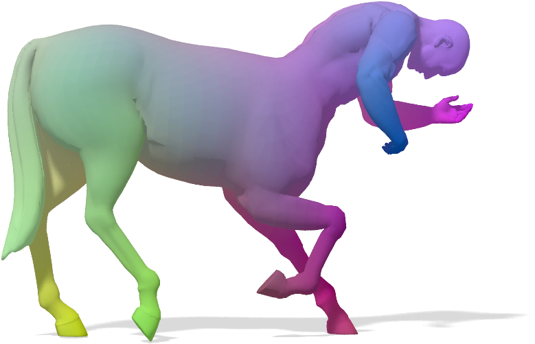
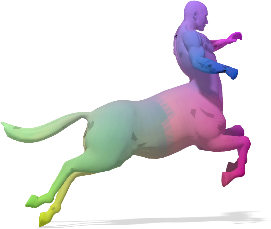
TOSCA. The TOSCA dataset [14] contains 76 shapes divided into 8 classes (humans and animals) of varying resolution (3K to 50K vertices). We match each shape with one instance of the same class. For shapes having more than 10K vertices we use our multiscale acceleration with an initial problem size of 10K and a maximum problem size of 3K for all further iterations. The parameters were set to $\alpha=10^{-10}$ and $t=[300\ 100\ 50\ 10]$, with 5 iterations per diffusion time. Figure 9 shows a quantitative evaluation.

Figure 9: Correspondence accuracy on the TOSCA dataset.

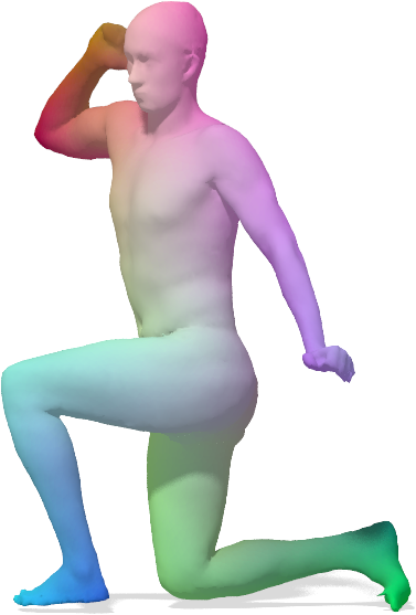
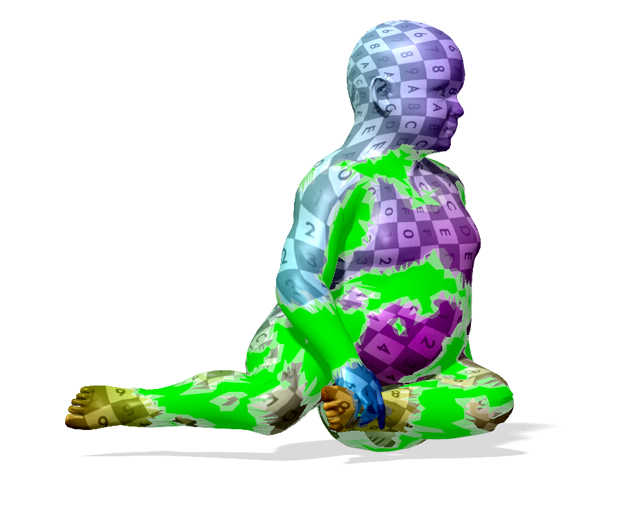
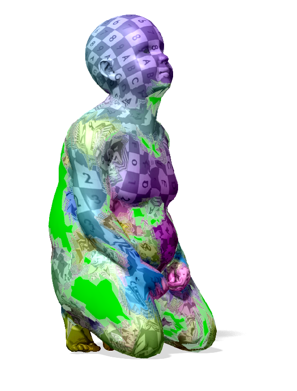
SCAPE. The SCAPE dataset [3] contains 72 clean shapes of scanned humans in different poses. For this test we set $\alpha=10^{-7}$, $t=[0.1\ 0.05\ 0.009\ 0.001\ 0.0001]$, and 5 iterations per diffusion time. We used multiscale acceleration with initial size equal to 10K vertices, and equal to 1K for subsequent iterations. Quantitative and qualitative results are given in Figure 8 and 1 (right) respectively.

FAUST. The FAUST dataset [7] contains 100 human scans belonging to 10 different individuals; for these tests we used the template subset of FAUST, consisting of shapes with around 7K vertices each. This allowed us to run our algorithm without multiscale acceleration. We set $\alpha=10^{-7}$ and $t=[500\ 323\ 209\ 135\ 87\ 36\ 23\ 15\ 10]$. Differently from the previous experiments, here we employ our method as a refinement step for several deep learning-based methods, demonstrating significant improvements (up to $50\%$) upon the ‘raw’ output of such approaches. The results are reported in Figure 10. Our results contain a few shapes in which body parts were swapped, preventing us from reaching 100%. An example is presented in the supp. material.

Figure 10: Correspondence accuracy on FAUST. Dashed curves indicate the performance of recent deep learning methods, solid curves are obtained using our method as post-processing. Our method based on handcrafted descriptors (SHOT) is denoted as ‘Handcrafted+Ours’.

Figure 11: Correspondence accuracy on SHREC’16 Topology.

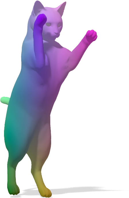
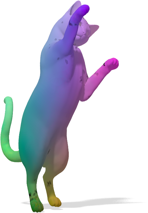
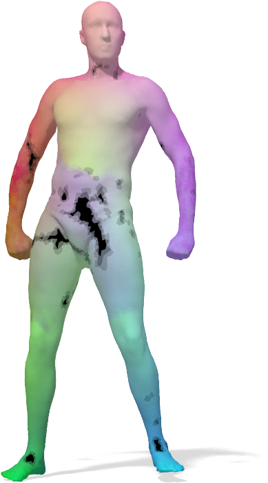
SHREC’16 Topology. This dataset [25] contains 25 shapes of the same class with around 12K vertices, undergoing near-isometric deformations in addition to large topological shortcuts (see Figure 1 middle). Here we use only SHOT as a descriptor, since HKS is not robust against topological changes. We used $\alpha=10^{-6}$ and $t=[2.7\ 2.44\ 2.1\ 1.95\ 1.7]$, using multiscale with an initial problem of size 12k and the following problems with maximum size 1k. Quantitative results are reported in Figure 11.

6 Conclusions

We considered a formulation of the problem of finding a smooth, possibly partial, correspondence between two non-isometric shapes as a quadratic assignment problem matching between point-wise and pair-wise descriptors. We showed that when choosing the pair-wise descriptors to be positive-definite kernel matrices (unlike the traditionally used distance matrices), the NP-hard QAP admits an exact relaxation over the space of bistochastic matrices, which we proposed to solve using a projected descent procedure motivated by the DC algorithm. The resulting iterations take the form of LAPs, which are solved using a multi-scale version of the auction algorithm. We interpreted the proposed algorithm as an alternating diffusion process, as iterated blurring and sharpening, and as a kernel density estimation procedure. The algorithm scales very well to even hundreds of thousands of vertices, and produces surprisingly good results. Experimental evaluation on various datasets shows that our method significantly improves the output obtained by the best existing correspondence methods.

Acknowledgements

This work has been supported by the ERC grants 307047 (COMET), 335491 (RAPID), 649323 (3D Reloaded) and 724228 (LEMAN).

Supplementary Material

Appendix A Details about the DC algorithm

In Section 3 of the submission we propose to use the DC algorithm to optimize

$$\arg\!\!\min_{\mathbf{P}\in\mathbb{R}^{n\times n}}B(\mathbf{P})-E(\mathbf{P}).$$ (95)

where $B$ is the convex indicator function of the set of bistochastic matrices $\mathcal{B}_{n}$ and $E$ is strictly convex and differentiable. We will now prove that the two steps

• Select $\mathbf{Q}^{k}\in\partial E(\mathbf{P}^{k})$

• Select $\mathbf{P}^{k+1}\in\partial B^{*}(\mathbf{Q}^{k})$.

of the DC algorithm are equivalent to

$$\mathbf{P}^{k+1}=\arg\!\!\max_{\mathbf{P}\in\mathcal{B}_{n}}\langle\mathbf{P},\nabla E(\mathbf{P}^{k})\rangle\,,$$ (96)

that each iterate $\mathbf{P}^{k}$ can be chosen to be a permutation matrix, and that $E(\mathbf{P}^{k})$ is a strictly increasing.

We assume that the reader is familiar with the concepts of convex conjugates and sub-gradients and just recall the following Lemma

Lemma 2.

Let $X$ be a Banach space and $f:X\rightarrow(-\infty,\infty]$ with $\partial f\neq\emptyset$. Then $f^{**}(x)=f(x)$ and

$$x^{*}\in\partial f(x) \Leftrightarrow x\in\partial f^{*}(x^{*})$$ (97)

Moreover for convex functions $f$, $0\in\partial f(x)$ is equivalent to

$$x =\arg\!\!\min_{x}f(x)$$ (98)

Let now $E$ be convex differentiable and $B$ the (convex) indicator function of a convex set $C$. We will derive equivalent expressions for the two steps in the DC algorithm for solving (95). Since $E$ is differentiable, its subdifferential at any point has one element, namely the gradient at that point:

$$\mathbf{Q}^{k}\in\partial E(\mathbf{P}^{k}) \Leftrightarrow\mathbf{Q}^{k}=\nabla E(\mathbf{P}^{k})$$ (99)

The second step $\mathbf{P}^{k+1}\in\partial B^{*}(\mathbf{Q}^{k})$ can be rewritten using Lemma 2:

$$\mathbf{P}^{k+1}\in\partial B^{*}(\mathbf{Q}^{k}) \Leftrightarrow\mathbf{Q}^{k}\in\partial B(\mathbf{P}^{k+1})$$

$$\Leftrightarrow 0\in-\mathbf{Q}^{k}+\partial B(\mathbf{P}^{k+1})$$

$$\Leftrightarrow\mathbf{P}^{k+1}=\arg\!\!\min_{\mathbf{P}}-\langle\mathbf{Q}^{k},\mathbf{P}\rangle+B(x)$$

$$\Leftrightarrow\mathbf{P}^{k+1}=\arg\!\!\max_{\mathbf{P}\in C}\langle\mathbf{Q}^{k},\mathbf{P}\rangle$$ (100)

Thus the DC algorithm in this special case reads

$$\mathbf{P}^{k+1}=\arg\!\!\max_{\mathbf{P}\in C}\langle\mathbf{P},\nabla E(\mathbf{P}^{k})\rangle\,.$$ (101)

In our case the convex set $C$ is the polyhedron $\mathcal{B}_{n}$ of bistochastic matrices. Since linear functions defined on a polyhedron attain their extrema at the vertices of the polyhedron, we can choose the maximizer to be a permutation matrix.

Due to the strict convexity of $E$ we further see:

$$E(\mathbf{P}^{k+1}) >E(\mathbf{P}^{k})+\langle\mathbf{P}^{k+1}-\mathbf{P}^{k},\nabla E(\mathbf{P}^{k})\rangle$$

$$\geq E(\mathbf{P}^{k})+\langle\mathbf{P}^{k}-\mathbf{P}^{k},\nabla E(\mathbf{P}^{k})\rangle$$

$$=E(\mathbf{P}^{k})$$ (102)

where the strong inequality holds until convergence and the weak inequality follows directly from (101).

Figure 12: A failure case of our method. Left and right are switched on the upper body, causing a non-continuous correspondence. We observed eight such failure cases in the entire FAUST dataset.

Appendix B Details on multiscale acceleration

The multiscale algorithm begins by solving for an initial sparse bijection $\pi_{0}:\mathcal{X}_{0}\to\mathcal{Y}_{0}$ between $n_{0}$ samples $s_{\mathcal{X}},s_{\mathcal{Y}}$ (also called seeds), obtained with farthest point sampling (Euclidean in our experiments). $n_{0}$ can either be the maximum amount of vertices that can be handled (around 15k in our experiments) or smaller if runtime is crucial. Then $s_{\mathcal{X}}$ is divided into $n_{0}/(k\cdot maxP)$ Voronoi cells $V_{\mathcal{X},0}$ and these Voronoi cells are transferred to $\mathcal{Y}$ using $\pi_{0}$ to create $V_{\mathcal{Y},0}$. The parameter $maxP$ is the maximum problem size allowed in later iterations and normally much smaller than $n_{0}$. $k$ determines how many new samples are added in each iteration. A small $maxP$ makes the method faster but less robust, and a small $k$ slower but more robust. In our experiments, we always choose $maxP=1500$ and $k=3$. At the first iteration ($i=1$) and any following iteration $i$, $n_{i}=k\times n_{i-1}$ new points are sampled in a farthest point manner on both shapes to create $\mathcal{X}_{i},\mathcal{Y}_{i}$. Each new point is assigned to the same Voronoi cell as its nearest neighbor in $s_{\mathcal{X}},s_{\mathcal{Y}}$ resulting in the new cells $V_{\mathcal{X},i},V_{\mathcal{Y},i}$. If any cell has more than $maxP$ vertices, the number of cells is increased until this is not the case anymore. Next we solve for $\pi_{i}:\mathcal{X}_{i}\to\mathcal{Y}_{i}$ by solving for a mapping from the $m$-th cell of $V_{\mathcal{X},i}$ to the $m$-th of $V_{\mathcal{X},i}$ using the proposed method from this paper and combining them into a global permutation. Notice that the $m$-th cells of both shapes correspond to roughly the same areas as long as the previous matching $\pi_{i-1}$ that was used for its construction is reasonable. Nevertheless, the cells could include a different amount of points due to discretization errors, so we need to apply the partial matching scheme for each cell and some points may stay unmatched (in this iteration). All matched points are added to the sets $s_{\mathcal{X}},s_{\mathcal{Y}}$ for the next iteration. Again, $\mathcal{X}$ is divided into $n_{i}/(k\cdot maxP)$ Voronoi cells and these are transfered to $\mathcal{Y}$ via $\pi_{i}$. The Voronoi cells of previous iterations are discarded to allow exchange of points between cells. This proceeds until all points have been sampled.

We use Euclidean FPS in all cases and build approximate Voronoi cells on remeshed versions of the shape to keep the runtime small. Each $\pi_{i}$ is solved for by using descriptors and initial matches from the previous iteration in the same cell. Additionally, we add $1000$ equally distributed matches from $\pi_{0}$ to every problem which aligns the solution along the boundaries of the cells with each other. Notice that even if the shapes have the same number of vertices at the beginning due to the sampling and decoupling of each cell not all vertices might be matched.

If the matched shapes are partial versions of each other, this information needs to be propagated from the first iteration on since all later cells are solved independently and can therefore not see partiality. In this case, $n_{0,\mathcal{X}},n_{0,\mathcal{Y}}$ can be chosen dependently on the ratio of areas or number of vertices between $\mathcal{X}$ and $\mathcal{Y}$, either assuming the scale or the discretization is comparable. Then certain points of the initial sampling will stay unmatched and be marked forbidden. They are handled exactly like any other seed but have their own Voronoi cell and any point that gets a assigned to the forbidden Voronoi cell is also marked forbidden such that the information spreads only to the neighborhood.

Appendix C Run time comparison

shapes in experiment	#vertices	runtime with heat kernel in sec	runtime with Gaussian kernel in sec
Tosca: cat0 to cat2	3400	29.25	97.77
Tosca: dog0 to dog2	3400	36	98.43
Tosca: centaur0 to centaur1	3400	25.31	98.91
Tosca: wolf0 to wolf1	4344	60.7	192.72
Faust models: 000 to 098	6890	109.477019	639.9
Faust models: 001 to 031	6890	104.68	609.56
Faust models: 002 to 039	6890	104.5	611.24
Faust models: 003 to 021	6890	106.41	614.23
Faust models: 004 to 033	6890	106.28	652.58

Table 1: Runtime comparison of matching between shapes with different number of vertices using heat kernels and Gaussian kernels.

The run time experiments, were conducted on a MacBook pro with a $2.5$ GHz Intel Core i7 processor and $16$ GB RAM running Matlab $2016b$. The experiments were conducted using $9$ pairs of shapes with a varying number of vertices from the TOSCA high and low resolution meshes as well as FAUST registrations set. The complete results are presented in Table 1. We ran all our tests using SHOT descriptors, 10 iterations with $\alpha=1/10^{8}$, $400$ eigenvectors to construct the heat kernels and a logarithmic scale of time parameters between $400$ and $10$.

Figure 13: Matching from a horse to an elephant using SHOT and HKS descriptors. The shapes are sampled in a way such that a bijective matching is possible.

Appendix D More results, Failure cases

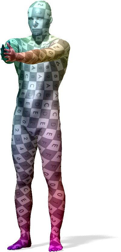
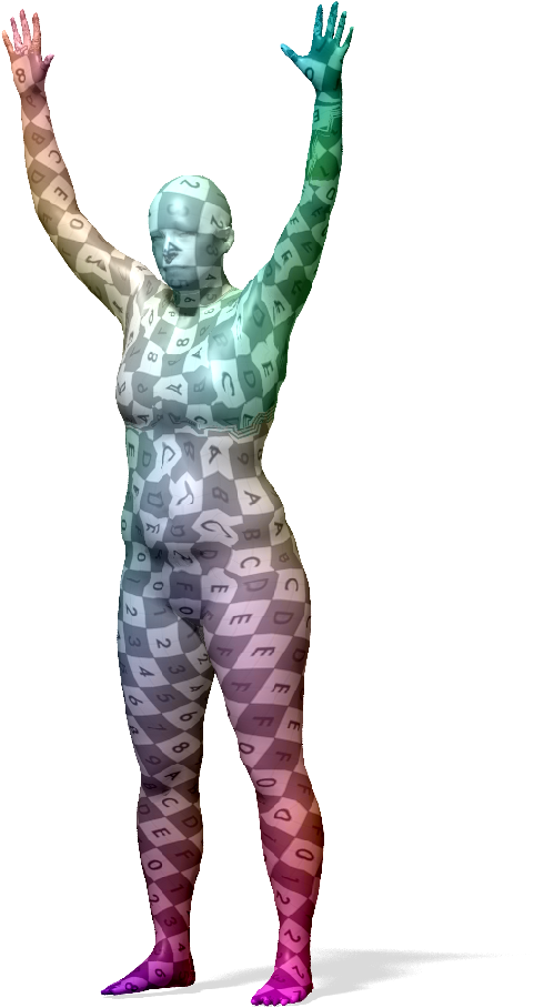
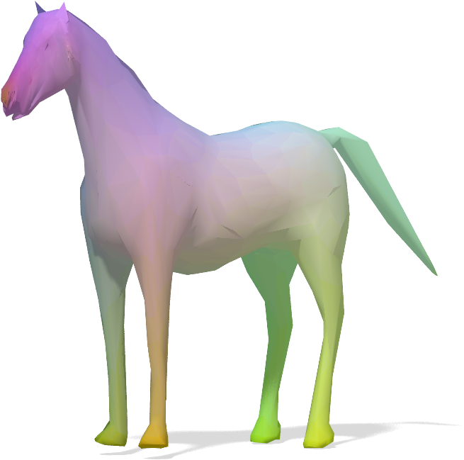
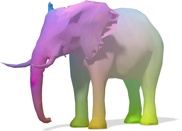
In this section we show additional results for a pair of dramatically non-isometric shapes (Fig.13), pairs from the Tosca dataset (Fig.14) and failure cases (Figs.12,15).

Figure 14: (left) A matching between two cats from the Tosca dataset. The unmatched points resulting from the multiscale (black) are very sparse. (right) A failed matching on the centaurs from Tosca. The front legs are swapped but only few points are unmatched.

Figure 15: (left) Failure case on the SCAPE dataset.The legs are mapped front to back causing a non continuous correspondence on the torso. Large unmatched areas due to the multiscale also appear there. Over the knees unaligned cell boundaries are visible. (right) Failure case on the SHREC’16 dataset. Many parts are missing or the texture is heavily distorted. These are really challenging shapes to match because the hands and feet are topologically merged to different parts of the body in both cases.

References

- [1] Y. Aflalo, A. Bronstein, and R. Kimmel. On convex relaxation of graph isomorphism. PNAS, 112(10):2942–2947, 2015.
- [2] Y. Aflalo, A. Dubrovina, and R. Kimmel. Spectral generalized multi-dimensional scaling. IJCV, 118(3):380–392, 2016.
- [3] D. Anguelov, P. Srinivasan, D. Koller, S. Thrun, J. Rodgers, and J. Davis. SCAPE: shape completion and animation of people. Proc. of ACM SIGGRAPH, 2005.
- [4] M. Aubry, U. Schlickewei, and D. Cremers. The wave kernel signature: A quantum mechanical approach to shape analysis. In Proc. 4DMOD, 2011.
- [5] D. P. Bertsekas. Network Optimization: Continuous and Discrete Models. Athena Scientific, 1998.
- [6] P. J. Besl and N. D. McKay. A method for registration of 3-d shapes. IEEE Transactions on Pattern Analysis and Machine Intelligence, 14(2):239–256, Feb 1992.
- [7] F. Bogo, J. Romero, M. Loper, and M. J. Black. FAUST: Dataset and evaluation for 3D mesh registration. In Proc. CVPR, 2014.
- [8] E. Bogomolny, O. Bohigas, and C. Schmit. Spectral properties of distance matrices. J. Physics A, 36(12):3595, 2003.
- [9] D. Boscaini, J. Masci, S. Melzi, M. M. Bronstein, U. Castellani, and P. Vandergheynst. Learning class-specific descriptors for deformable shapes using localized spectral convolutional networks. Computer Graphics Forum, 34(5):13–23, 2015.
- [10] D. Boscaini, J. Masci, E. Rodolà, and M. M. Bronstein. Learning shape correspondence with anisotropic convolutional neural networks. In Proc. NIPS, 2016.
- [11] D. Boscaini, J. Masci, E. Rodolà, M. M. Bronstein, and D. Cremers. Anisotropic diffusion descriptors. In Computer Graphics Forum, volume 35, pages 431–441, 2016.
- [12] A. M. Bronstein, M. M. Bronstein, and R. Kimmel. Efficient computation of isometry-invariant distances between surfaces. SIAM J. Sci. Comp., 28(5):1812–1836, 2006.
- [13] A. M. Bronstein, M. M. Bronstein, and R. Kimmel. Generalized multidimensional scaling: a framework for isometry-invariant partial surface matching. PNAS, 103(5):1168–1172, 2006.
- [14] A. M. Bronstein, M. M. Bronstein, and R. Kimmel. Numerical geometry of non-rigid shapes. Springer, 2008.
- [15] A. M. Bronstein, M. M. Bronstein, R. Kimmel, M. Mahmoudi, and G. Sapiro. A Gromov-Hausdorff framework with diffusion geometry for topologically-robust non-rigid shape matching. IJCV, 89(2):266–286, 2010.
- [16] M. M. Bronstein and I. Kokkinos. Scale-invariant heat kernel signatures for non-rigid shape recognition. In Proc. CVPR, 2010.
- [17] Q. Chen and V. Koltun. Robust nonrigid registration by convex optimization. In Proc. ICCV, pages 2039–2047, 2015.
- [18] R. R. Coifman, S. Lafon, A. B. Lee, M. Maggioni, B. Nadler, F. Warner, and S. W. Zucker. Geometric diffusions as a tool for harmonic analysis and structure definition of data: Diffusion maps. PNAS, 102(21):7426–7431, 2005.
- [19] A. Elad and R. Kimmel. On bending invariant signatures for surfaces. Trans. PAMI, 25(10):1285–1295, 2003.
- [20] N. Hu and L. Guibas. Spectral descriptors for graph matching. arXiv preprint arXiv:1304.1572, 2013.
- [21] I. Kezurer, S. Z. Kovalsky, R. Basri, and Y. Lipman. Tight relaxation of quadratic matching. In Computer Graphics Forum, volume 34, pages 115–128, 2015.
- [22] V. G. Kim, Y. Lipman, and T. A. Funkhouser. Blended intrinsic maps. Trans. Graphics, 30(4), 2011.
- [23] A. Kovnatsky, M. M. Bronstein, X. Bresson, and P. Vandergheynst. Functional correspondence by matrix completion. In Proc. CVPR, 2015.
- [24] A. Kovnatsky, M. M. Bronstein, A. M. Bronstein, K. Glashoff, and R. Kimmel. Coupled quasi-harmonic bases. Computer Graphics Forum, 32(2):439–448, 2013.
- [25] Z. Lähner, E. Rodolà, M. M. Bronstein, D. Cremers, O. Burghard, L. Cosmo, A. Dieckmann, R. Klein, and Y. Sahillioglu. SHREC’16: Matching of deformable shapes with topological noise. In Proc. 3DOR, 2016.
- [26] R. R. Lederman and R. Talmon. Learning the geometry of common latent variables using alternating-diffusion. App. and Comp. Harmonic Analysis, 2015.
- [27] M. Leordeanu and M. Hebert. A spectral technique for correspondence problems using pairwise constraints. In Proc. ICCV, 2005.
- [28] Y. Lipman and T. Funkhouser. Möbius voting for surface correspondence. In Trans. Graphics, volume 28, page 72, 2009.
- [29] O. Litany, T. Remez, E. Rodolà, A. M. Bronstein, and M. M. Bronstein. Deep functional maps: Structured prediction for dense shape correspondence. In Proc. ICCV, 2017.
- [30] O. Litany, E. Rodolà, A. Bronstein, and M. Bronstein. Fully spectral partial shape matching. Computer Graphics Forum, 36(2):1681–1707, 2017.
- [31] X. Liu, A. Donate, M. Jemison, and W. Mio. Kernel functions for robust 3d surface registration with spectral embeddings. In ICPR, pages 1–4, 2008.
- [32] J. Masci, D. Boscaini, M. M. Bronstein, and P. Vandergheynst. Geodesic convolutional neural networks on Riemannian manifolds. In Proc. 3DRR, 2015.
- [33] D. Mateus, R. Horaud, D. Knossow, F. Cuzzolin, and E. Boyer. Articulated shape matching using laplacian eigenfunctions and unsupervised point registration. In Proc. CVPR, 2008.
- [34] F. Mémoli and G. Sapiro. A theoretical and computational framework for isometry invariant recognition of point cloud data. Foundations of Computational Mathematics, 5(3):313–347, 2005.
- [35] F. Monti, D. Boscaini, J. Masci, E. Rodolà, J. Svoboda, and M. M. Bronstein. Geometric deep learning on graphs and manifolds using mixture model CNNs. In Proc. CVPR, 2017.
- [36] M. Ovsjanikov, M. Ben-Chen, J. Solomon, A. Butscher, and L. Guibas. Functional maps: a flexible representation of maps between shapes. Trans. Graphics, 31(4):30, 2012.
- [37] P. M. Pardalos, H. Wolkowicz, et al. Quadratic Assignment and Related Problems: DIMACS Workshop, May 20-21, 1993, volume 16. American Mathematical Soc., 1994.
- [38] D. Raviv, A. M. Bronstein, M. M. Bronstein, R. Kimmel, and N. Sochen. Affine-invariant geodesic geometry of deformable 3d shapes. Computers & Graphics, 35(3):692–697, 2011.
- [39] E. Rodolà, A. M. Bronstein, A. Albarelli, F. Bergamasco, and A. Torsello. A game-theoretic approach to deformable shape matching. In Proc. CVPR, 2012.
- [40] E. Rodolà, L. Cosmo, M. M. Bronstein, A. Torsello, and D. Cremers. Partial functional correspondence. Computer Graphics Forum, 36(1):222––236, 2017.
- [41] E. Rodolà, M. Moeller, and D. Cremers. Point-wise map recovery and refinement from functional correspondence. In Proc. VMV, pages 25–32, Aachen, Germany, 2015. Eurographics Association.
- [42] E. Rodolà, S. Rota Bulò, T. Windheuser, M. Vestner, and D. Cremers. Dense non-rigid shape correspondence using random forests. In Proc. CVPR, 2014.
- [43] R. M. Rustamov. Laplace-Beltrami eigenfunctions for deformation invariant shape representation. In Proc. SGP, 2007.
- [44] Y. Sahillioglu and Y. Yemez. Coarse-to-fine combinatorial matching for dense isometric shape correspondence. In Computer Graphics Forum, volume 30, pages 1461–1470, 2011.
- [45] Y. Sahillioğlu and Y. Yemez. Minimum-distortion isometric shape correspondence using EM algorithm. IEEE Trans. Pattern Anal. Mach. Intell., 34(11):2203–2215, 2012.
- [46] G. Shamai and R. Kimmel. Geodesic distance descriptors. CoRR, abs/1611.07360, 2016.
- [47] A. Shtern and R. Kimmel. Iterative closest spectral kernel maps. In Proc. 3DV, volume 1, pages 499–505. IEEE, 2014.
- [48] A. Shtern and R. Kimmel. Matching the lbo eigenspace of non-rigid shapes via high order statistics. Axioms, 3(3):300–319, 2014.
- [49] J. Sun, M. Ovsjanikov, and L. Guibas. A concise and provably informative multi-scale signature based on heat diffusion. In Computer Graphics Forum, volume 28, pages 1383–1392, 2009.
- [50] A. Tevs, A. Berner, M. Wand, I. Ihrke, and H.-P. Seidel. Intrinsic shape matching by planned landmark sampling. In Computer Graphics Forum, volume 30, pages 543–552, 2011.
- [51] F. Tombari, S. Salti, and L. Di Stefano. Unique signatures of histograms for local surface description. In Proc. ECCV, 2010.
- [52] L. Torresani, V. Kolmogorov, and C. Rother. Feature correspondence via graph matching: Models and global optimization. In Proc. ECCV, 2008.
- [53] M. Vestner, R. Litman, E. Rodolà, A. Bronstein, and D. Cremers. Product manifold filter: Non-rigid shape correspondence via kernel density estimation in the product space. Proc. CVPR, 2017.
- [54] C. Wang, M. M. Bronstein, A. M. Bronstein, and N. Paragios. Discrete minimum distortion correspondence problems for non-rigid shape matching. In Proc. SSVM, 2011.
- [55] T. Windheuser, U. Schlickewei, F. R. Schmidt, and D. Cremers. Geometrically consistent elastic matching of 3d shapes: A linear programming solution. In Proc. ICCV, 2011.