Parametrizing growth in dark energy and modified gravity models

Abstract

It is well-known that an extremely accurate parametrization of the growth function of matter density perturbations in $\Lambda$CDM cosmology, with errors below $0.25\%$, is given by $f(a)=\Omega_{m}^{\gamma}\,(a)$ with $\gamma\simeq 0.55$. In this work, we show that a simple modification of this expression also provides a good description of growth in modified gravity theories. We consider the model-independent approach to modified gravity in terms of an effective Newton constant written as $\mu(a,k)=G_{eff}/G$ and show that $f(a)=\beta(a)\Omega_{m}^{\gamma}\,(a)$ provides fits to the numerical solutions with similar accuracy to that of $\Lambda$CDM. In the time-independent case with $\mu=\mu(k)$, simple analytic expressions for $\beta(\mu)$ and $\gamma(\mu)$ are presented. In the time-dependent (but scale-independent) case $\mu=\mu(a)$, we show that $\beta(a)$ has the same time dependence as $\mu(a)$. As an example, explicit formalae are provided in the DGP model. In the general case, for theories with $\mu(a,k)$, we obtain a perturbative expansion for $\beta(\mu)$ around the General Relativity case $\mu=1$ which, for $f(R)$ theories, reaches an accuracy below $1\%$. Finally, as an example we apply the obtained fitting functions in order to forecast the precision with which future galaxy surveys will be able to measure the $\mu$ parameter.

I Introduction

One of the most important open problems in cosmology is to understand the physics behind cosmic acceleration Riess:1998cb ; Perlmutter:1998np ; Eisenstein:2005su ; Percival:2007yw . Most of the models proposed to date can be classified in two major categories, namely, dark energy and modified gravity. The former refers to a new component which acts as a source of gravity within the framework of General Relativity (GR), the simplest example being a cosmological constant. By modified gravity we understand extensions of GR which include new degrees of freedom that mediate the gravitational interaction. Well-known examples of these theories are the $f(R)$ models Nojiri:2003ft ; Capozziello:2003tk or the Dvali, Gabadadze y Porrati model (DGP) Dvali:2000hr .

The main source of observational information about cosmic acceleration comes from distance measurements which can map the expansion history of the universe. However, this kind of observations alone are not able to completely discriminate between the different theoretical approaches. In recent years the construction of large galaxy catalogues has opened the possibility of mapping not only the expansion but also the growth history of large-scale structures. In general, modified gravity theories change the relation between the density perturbations and the gravitational potentials, thus modifying the amplitude of matter density perturbations as a function of time (growth function). They also modify the equations determining the form of the gravitational potential entering in the photon propagation equation (lensing potential). Thus, observations of clustering and lensing at different redshifts provide a way to break the degeneracy between different acceleration models.

For the sake of concreteness, we will consider scalar perturbations around a flat FLRW background in the longitudinal gauge Tsujikawa ,

$$ds^{2}=-(1+2\Psi)dt^{2}+a^{2}(t)(1+2\Phi)d{\bf x}^{2}$$ (1)

At the background level, the model is characterized by its Hubble function $H(a)=\dot{a}/a$ which allows to determine the cosmological distances.

At the perturbation level, the modified Einstein equations in a wide range of gravity theories, for sub-Hubble scales and in the quasi-static approximation lead to a modified Poisson equation that in Fourier space reads

$$k^{2}\Psi\simeq-4\pi G_{\text{eff}}\,a^{2}\rho_{m}\delta_{m}$$ (2)

where $\delta_{m}=\delta\rho_{m}/\rho_{m}$ is the matter density contrast which is related to the galaxy density contrast $\delta_{g}$ by the bias factor $b$ as $\delta_{g}=b\,\delta_{m}$. Here $G_{\text{eff}}$ is the effective gravitational coupling which will differ in general from the bare gravitational constant $G=1/(8\pi M_{p}^{2})$. The growth equation reads

$$\delta^{\prime\prime}_{m}+\left(2+\frac{H^{\prime}}{H}\right)\delta^{\prime}_{m}-\frac{3}{2}\mu(a,k)\Omega_{m}(a)\delta_{m}\simeq 0$$ (3)

where prime denotes derivative with respect to $\ln a$ and $\Omega_{m}(a)$ is the matter density parameter $\Omega_{m}(a)=\Omega_{m}\,a^{-3}\,\frac{H_{0}^{2}}{H^{2}(a)}$.

Figure 1: From left to right: $\gamma$, $\beta$ and relative error in the growth function as a function of $\mu$. The dashed red line corresponds to analytical approximation in (20) with $\gamma=\gamma_{*}$ and $\beta$ in (19). The continuous blue line, corresponds to the numerical fitting of $\beta$ and $\gamma$ to expression (22).

On the other hand, the lensing potential satisfies

$$\frac{\Psi-\Phi}{2}\simeq-\frac{3G_{\text{eff}}}{2G}\frac{1+\eta}{2}\left(\frac{aH}{k}\right)^{2}\Omega_{m}(a)\delta_{m}$$ (4)

These modifications of Einstein equations are parametrized by two free functions:

$$\mu(a,k)=\frac{G_{\text{eff}}}{G}$$ (5)

and

$$\eta(a,k)=-\frac{\Phi}{\Psi}\,.$$ (6)

For any local and generally covariant four-dimensional theory of gravity, it can be shown that they reduce to rational functions of $k$ which are even in theories with purely scalar extra degrees of freedom. If we also assume that no higher than second derivatives appear in the equations of motions, then they can be completely described by five functions of time only as follows Silvestri:2013ne

$$\mu(a,k)=\frac{1+p_{3}(a)k^{2}}{p_{4}(a)+p_{5}(a)k^{2}}$$ (7)

and

$$\eta(a,k)=\frac{p_{1}(a)+p_{2}(a)k^{2}}{1+p_{3}(a)k^{2}}\,.$$ (8)

Thus, deviations from $\mu=\eta=1$ signal a breakdown of standard GR.

Once the evolution of perturbations have been solved, the growth function is defined as,

$$f(a)=\frac{d\,\ln(\delta_{m})}{d\,\ln(a)}.$$ (9)

In the case of $\Lambda$CDM, a good approximation for the growth function is given by,

$$f(a)=\Omega_{m}^{\gamma}(a),$$ (10)

where $\gamma$ is known as the growth index which has a value in $\Lambda$CDM of $\gamma_{*}\simeq 0.55$ Linder:2005 ; Linder:2007hg . This expression provides accuracies better than $0.25\%$, and accordingly could be useful in the data analysis of present and future surveys such as J-PAS J-PAS , DESI DESI or Euclid Euclid which will be able to measure $f(z)$ with precisions around $1\%-3\%$.

In the modified gravity case, (10) does not necessarily provide a good fit and different alternatives have been considered in the literature, mainly focused on the modification of the growth index. Such alternative expressions have been obtained on a case by case basis and to the best of our knowledge no model-independent analysis has been performed so far. Thus the aim of this work is to fill this gap and determine accurate fitting functions for the modified growth function in terms of the $\mu$ parameter in a model-independent way.

The paper is organized as follows: in section II we analyze the case in which $\mu\,(a,k)$ does not depend on redshift, and we find an approximate analytic expression for the growth function. In section III we consider the time-dependent but scale-independent case and apply our results to the DGP model. In IV, we propose a perturbative parametrization for the general case $\mu\,(a,k)$ and consider $f(R)$ theories as an example. In section V, we make use of the obtained fitting functions in order to forecast the precision with which future galaxy surveys will be able to measure the $\mu$ parameter in the redshift-independent case. Finally in section VI we briefly discuss the results and conclusions.

Figure 2: Errors for $f(z)$, $\delta_{m}(z)$ and $f(z)\delta_{m}(z)$ in $\Lambda$CDM using $\gamma_{*}=0.554$ (left) and $\gamma_{*}=0.550$ (right). We see that for $\gamma_{*}=0.554$ the error in $f(z)$ is below $0.25\%$ but that in $\delta_{m}(z)$ reaches $0.15\%$, whereas for $\gamma_{*}=0.550$, the error in $\delta_{m}(z)$ can be reduced below $0.05\%$, however the corresponding error for $f(z)$ grows to $0.7\%$.

II Time-independent case $\mu=\mu(k)$

We start by studying the simplest case in which functions $p_{i}(a)=p_{i}$ in (7) are constant so that $\mu\,(a,\,k)=\mu(k)$ does not depend on the scale factor. Although in general for modified gravities with extra scalar or vector degrees of freedom we expect both time and scale dependence of the $\mu$ factor, the time-independent case can be used for phenomenological parametrizations of the effective Newton constant at different length scales. It can also be applied in scalar-tensor models as Gannouji:2008jr in which $G_{eff}$ rapidly tends to a constant at high redshift.

In this simple case, we can develop an analytical study. Making the change of variable from $\delta_{m}$ to $f$ in equation (3) we have,

$$f^{\prime}+f^{2}+\left(2+\frac{H^{\prime}}{H}\right)\,f-\frac{3}{2}\,\mu\,(k)\,\Omega_{m}(a)=0.$$ (11)

Let us first assume for simplicity a $\Lambda$CDM background. Later on we will consider a more general case with time-dependent effective equation of state for the dark energy or modified gravity extra components. The Hubble parameter in $\Lambda$CDM reads,

$$H(a)=H_{0}\,\sqrt{\Omega_{m}\,a^{-3}+\Omega_{\Lambda}},$$ (12)

with this expression and taking into account the definition of $\Omega_{m}(a)$ in function of $H$, we can obtain,

$$\frac{H^{\prime}}{H}=-\frac{3}{2}\,\Omega_{m}(a),$$ (13)

and

$$\Omega_{m}^{\prime}(a)=-3\,\Omega_{m}(a)\,(1-\Omega_{m}(a)).$$ (14)

Inspecting the numerical solutions of (11), we can see that a parametrization that provides a good fit is of the form,

$$f(a,k)=\beta(k)\,\Omega_{m}^{\gamma(k)}(a),$$ (15)

where for each Fourier mode, $\beta(k)$ and $\gamma(k)$ are in general the constants to adjust. This parametrization type was considered in DiPorto:2007ovd for the particular case of a scalar-tensor theories. Using equations (13) and (14) together with (15) in equation (11) we have,

$$(2-3\gamma)\,\Omega_{m}^{\gamma-1}(a)+\left(3\gamma-\frac{3}{2}\right)\,\Omega_{m}^{\gamma}(a)$$

$$+\beta\,\Omega_{m}^{2\gamma-1}(a)-\frac{3}{2}\,\frac{\mu}{\beta}=0.$$ (16)

Although this expression can be satisfied exactly only in the case in which $\Omega_{m}(a)=\Omega_{m}$ is a constant, as commented before, it is possible to obtain approximate solutions in the general case. Thus, for example, substituting $\mu=\beta=1$, we recover the case of $\Lambda$CDM so that for $\gamma=\gamma_{*}$ equation (II) is satisfied so that,

$$(2-3\gamma_{*})\,\Omega_{m}^{\gamma_{*}-1}(a)+(3\gamma_{*}-3/2)\,\Omega_{m}^{\gamma_{*}}(a)$$

$$+\Omega_{m}^{2\gamma_{*}-1}(a)-\frac{3}{2}\simeq 0,$$ (17)

Thus, if we take $\gamma=\gamma_{*}$ in the case with $\mu$ and $\beta$ different from one, we get from (II) and (II)

$$3\left(1-\frac{\mu}{\beta}\right)+2(\beta-1)\,\Omega_{m}^{2\gamma_{*}-1}(a)\simeq 0.$$ (18)

We consider a final approximation. Since $\gamma_{*}\simeq 1/2$, we assume that $\Omega_{m}^{2\gamma_{*}-1}(a)\simeq 1$. Thus we are able to find a relationship between $\mu$ and $\beta$,

$$\beta=\frac{1}{4}\,\left[\sqrt{1+24\,\mu}-1\right].$$ (19)

Therefore, we have an analytic expression which is an approximate solution of equation (11) for redshift-independent $\mu(k)$

$$f(a,k)=\frac{1}{4}\,\left[\sqrt{1+24\,\mu(k)}-1\right]\,\Omega_{m}^{\gamma_{*}}(a).$$ (20)

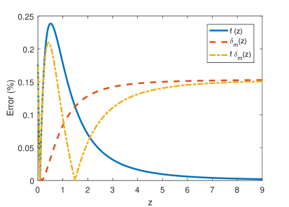
The error of this approximation generally depends on the scale factor and reaches a maximum at $a=1$ as discussed below. In Fig. 1, we plot the maximum error as a function of $\mu$ for $\Omega_{m}=0.271$. We have taken this particular value in order to compare with previous works although we have checked that the results remain unchanged in the range $\Omega_{m}=0.27-0.31$ which includes the latest Planck value Planck . The error corresponds to the difference between the fitting function and the numerical solution of (11) divided by their average value. We can see that the error is always below $2\%$. Notice that we have considered a wide range of $\mu$ values, although relatively small deviations from $\mu=1$ could generate a large integrated Sachs-Wolfe effect.

Figure 3: From left to right, functions $\gamma\,(\mu)$ (31), $\beta\,(\mu)$ (19) and growth function relative error, for time-independent $\mu$ for different values of $\omega_{0}$ with $\omega_{1}=0$. We have assumed that $\Omega_{m}=0.271$.

Figure 4: From left to right, functions $\gamma\,(\mu)$ (31), $\beta\,(\mu)$ (19) and growth function relative error, for time-independent $\mu$ for different values of $\omega_{1}$ with $\omega_{0}=-1$. We have assumed that $\Omega_{m}=0.271$.

It is however possible to improve the fit if we allow also the growth index $\gamma$ to depend on $\mu$. In this case, it is possible to find a good agreement with

$$\gamma\,(\mu)=\frac{1}{2}+\frac{0.161}{1.967+\beta\,(\mu)},$$ (21)

with $\beta(\mu)$ given in (19). In Fig. 1 we plot this relation together with the error corresponding to the improved growth function

$$f(a,k)=\frac{1}{4}\,\left[\sqrt{1+24\,\mu(k)}-1\right]\,\Omega_{m}^{\gamma(\mu(k))}(a).$$ (22)

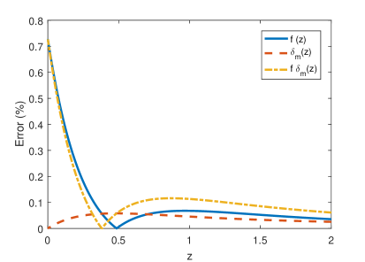
We can see that in this case, the maximum error can be below $0.25\%$. Also, we see that for GR ($\mu=1$), we obtain $\gamma_{*}=0.554$ as the value for the best fit, which is slightly different from that quoted in Linder:2005 ($\gamma_{*}=0.550$). In order to understand the difference, we analyze the error in three different functions, $f(z)$, $\delta_{m}(z)$ and $f(z)\delta_{m}(z)$ (see also Linder2 ). As we can see in Fig. 2, the error in $f(z)$ is larger for low redshift than the error in $\delta_{m}(z)$, but in general the errors for the three functions are of the same order. Notice that the value $\gamma_{*}=0.554$ minimizes the error in $f(z)$, however, the error in $\delta_{m}(z)$ is minimized by $\gamma_{*}=0.550$ Linder:2005 . This value also minimizes the error both in $f(z)$ and $f(z)\delta_{m}(z)$ for $z>0.4$ Since the error in the observable $f(z)\sigma_{8}(z)$ is dominated by the error in $f(z)$ we have taken $\gamma_{*}=0.554$ as our reference value in this work.

On the other hand, at early times, in the matter dominated era, $\Omega_{m}(a)\simeq 1$ and equation (11) can be solved exactly

$$f(a,k)=\frac{1}{4}\,\left[\sqrt{1+24\,\mu(k)}-1\right],$$ (23)

therefore $f(a,k)$ is just constant in time. The fitting function (20) exactly agrees with this result for $\Omega_{m}(a)=1$ and this is the reason why the error increases as we move away from the matter era. Thus for matter domination the density contrast grows as

$$\delta_{m}(a,k)\propto a^{\frac{1}{4}\,\left[\sqrt{1+24\,\mu(k)}-1\right]},$$ (24)

in agreement with Fry ; Gannouji:2008jr . This implies that if we want to preserve the growth of density contrast proportional to the scale factor in the matter era, $\mu$ should depend on the scale factor and tend to unity at early times.

Figure 5: Relative difference between the numerical solution and the fitting function (34) for the model $\mu\,(a)=1+b\,a$. As we see, the maximum error is reached at $z=0$.

II.1 Beyond the $\Lambda$CDM background

We now consider modifications of the background expansion. In order to keep the approach model-independent, we will parametrize them with an extra component $\Omega_{DE}(a)$ with arbitrary equation of state $\omega_{DE}(a)$. This extra component could correspond directly to dark energy or to the effective fluid description of the modified gravity. At late times, i.e. neglecting the radiation contribution, we can write

$$H(a)=H_{0}\,\sqrt{\Omega_{m}\,a^{-3}+\Omega_{DE}(a)},$$ (25)

with

$$\Omega_{DE}(a)=\Omega_{DE}\,\exp\left(\int_{0}^{a}\frac{3(1+\omega_{DE}(\hat{a}))}{\hat{a}}d\hat{a}\right).$$ (26)

Using (25) to obtain $\Omega_{m}(a)$, we get the expressions that replace (13) and (14),

$$\frac{H^{\prime}}{H}=-\frac{3}{2}\,\Omega_{m}(a)+\frac{\Omega_{m}(a)}{2\,\Omega_{m}}\,a^{3}\,\Omega_{DE}^{\prime}(a),$$ (27)

and

$$\Omega_{m}^{\prime}(a)=-3\,\Omega_{m}(a)\,(1-\Omega_{m}(a))-\frac{\Omega_{m}^{2}(a)}{\Omega_{m}}\,a^{3}\,\Omega_{DE}^{\prime}(a).$$ (28)

Following the same procedure as above, we obtain the analogous equation to (II) with an extra term,

$$(2 - 3\gamma)\,\Omega_{m}^{\gamma-1}(a)+\left(3\gamma-\frac{3}{2}\right)\,\Omega_{m}^{\gamma}(a)$$ (29)

$$+ \beta\,\Omega_{m}^{2\gamma-1}(a)-\frac{3}{2}\,\frac{\mu}{\beta}$$

$$+ \left(\frac{1}{2}-\gamma\right)\frac{\Omega_{DE}^{\prime}(a)}{\Omega_{m}}\,a^{3}\,\Omega_{m}^{\gamma}(a)=0.$$

We see that the new term is proportional to $(\frac{1}{2}-\gamma)$, so it is expected that it does not increase the errors in an important manner. Thus, considering the fitting function with $\gamma=\gamma_{*}$ in (20), we can see, that the errors increase in comparison with those for the $\Lambda$CDM background up to $3\%$.

As we did in the $\Lambda$CDM case, we can obtain better fits by modifying the expressions for $\beta(k)$ and $\gamma(k)$. Thus, the analysis shows that $\beta(k)$ is not sensitive to $\omega_{DE}(a)$ and therefore (19) provides a good approximation also in this case. The expression for $\gamma$ is however modified.

For example for the effective equation of state given by Chevallier:2000qy ; Linder:2002et ,

$$\omega_{DE}(a)=\omega_{0}+\omega_{1}\,(1-a).$$ (30)

with $\omega_{0}$ and $\omega_{1}$ constants, we find

$$\gamma(\mu,\omega_{0},\omega_{1})=\frac{1}{2}+\frac{0.161}{\beta(\mu)-1.967\omega_{0}-0.4789\omega_{1}}$$ (31)

Thus, the growth function reads in this case

$$f(a,k)=\frac{1}{4}\,\left[\sqrt{1+24\,\mu(k)}-1\right]\,\Omega_{m}^{\gamma(\mu(k),\omega_{0},\omega_{1})}(a).$$ (32)

In Fig. 3 and Fig. 4 we can see that the error can be reduced to $0.5\%$ with this parametrization.

Figure 6: Numerical solutions in the model $\mu\,(a)=1+b\,a$ for different values of $b$. The fit according to the equation (34) is not represented because it differs in less than $0.6\,\%$ with respect to the numerical solution.

Figure 7: From left to right, the functions $\gamma\,(\Omega_{0})$, $\Omega_{0}^{*}\,(\Omega_{0})$ and the relative error of the growth function for the DGP model. The error decreases as we increase the value of $\Omega_{0}$. The maximum error is less than $0.5\,\%$ for typical values of $\Omega_{0}$.

III scale-independent case $\mu=\mu(a)$

We have just seen that in the time-independent $\mu$ case, an ansatz of the form,

$$f(a)=\beta\;\Omega_{m}^{\gamma}(a),$$ (33)

provides a good fit to the numerical solutions. Let us now consider the case in which $\mu=\mu\,(a;p_{1},...,p_{n})$ where $[p_{1},...,p_{n}]$ are the set of $n$ cosmological parameters that $\mu$ depends on, i.e. $\mu$ can depend on redshift(time) but not on the scale $k$. We will explore a similar ansatz for the growth function,

$$f(a)=\beta\,(a;p^{*}_{1},...,p^{*}_{n})\,\Omega_{m}^{\gamma}(a),$$ (34)

where, in general, $p^{*}_{i}=p^{*}_{i}(p_{1},...,p_{n})$, $\gamma=\gamma(p_{1},...,p_{n})$ and let us assume that the $\beta$ function has the same $a$-dependence as the $\mu$ function (see Dent:2009wi ; BuenoSanchez:2010wd for similar proposals in particular models).

Thus, let us consider a simple example. For instance if $\mu\,(a)=1+b\,a$ being $b$ dimensionless constant, then we consider $\beta=1+b^{*}a$, with $b^{*}=b^{*}(b)$.

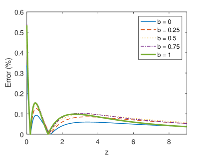
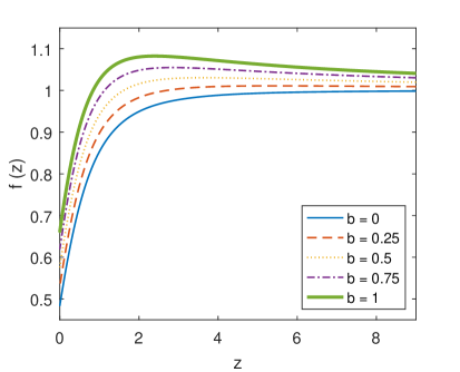
In Fig. 5 we show the fit error for different values of $b$. In Fig. 6 we can see the growth functions for the corresponding values of $b$. A $\Lambda$CDM background with $\Omega_{m}=0.271$ has been assumed. It can be seen how it grows with redshift reaching values larger than one and then decreases tending to one when matter starts dominating. We can see that in this simple example, the parametrization (34) provides fitting errors below $0.5\%$ in the whole redshift range, but they are even below $0.2\%$ for $z>0.1$ .

After we have studied this simple model, and checked the usefulness of parametrization (34), we will apply it to more realistic models of modified gravity, such as DGP and certain phenomenological parametrizations of $\mu\,(a)$.

Figure 8: From left to right, the functions $\gamma\,(\mu_{0})$, $\mu_{0}^{*}\,(\mu_{0})$ and relative error of the growth function for the phenomenological model (43) for different values of $\omega_{0}$, setting $\omega_{1}=0$. The case with $\omega_{0}=-1$ is parametrized in (III.2) and (47).

Figure 9: From left to right, the functions $\gamma\,(\mu_{0})$, $\mu_{0}^{*}\,(\mu_{0})$ and relative error of the growth function for the phenomenological model (43) for different values of $\omega_{1}$, setting $\omega_{0}=-1$. The case with $\omega_{1}=0$ is parametrized in (III.2) and (47).

III.1 DGP Model

In the DGP model Dvali:2000hr , the background evolution differs from $\Lambda$CDM so that

$$\Omega_{m}\,(a)=\frac{\Omega_{0}\,a^{-3}}{[(1-\Omega_{0})/2+\sqrt{\Omega_{0}\,a^{-3}+(1-\Omega_{0})^{2}/4}]^{2}},$$ (35)

and

$$\frac{H^{\prime}}{H}=-\frac{3\,\Omega_{m}(a)}{1+\Omega_{m}(a)}.$$ (36)

being $\Omega_{0}=\Omega_{m}(a=1)$ the only free parameter at the background level. The modified gravity parameters in this case read Kunz

$$\mu\,(a)=\frac{2(1+2\,\Omega_{m}^{2}\,(a))}{3(1+\Omega_{m}^{2}\,(a))}$$ (37)

and

$$\eta\,(a)=\frac{2+\Omega_{m}^{2}(a)}{1+2\,\Omega_{m}^{2}(a)}.$$ (38)

which are both $k$-independent, so that we try the parametrization in (34).

Thus, using (35), (36) and (37) in equation (3), solving numerically and fitting to (34), we get

$$f(a)=\frac{2(1+2\,\Omega_{m}^{2}\,(a;\,\Omega^{*}_{0}))}{3(1+\Omega_{m}^{2}\,(a;\,\Omega^{*}_{0}))}\,\Omega_{m}^{\gamma(\Omega_{0})}(a),$$ (39)

where $\Omega_{m}\,(a;\,\Omega^{*}_{0})$ follows equation (35) replacing $\Omega_{0}$ by $\Omega^{*}_{0}$. So we have two parameters to fit $\Omega^{*}_{0}\,(\Omega_{0})$ and $\gamma\,(\Omega_{0})$, which are given by the following expressions

$$\Omega^{*}_{0}(\Omega_{0})=0.8\,\Omega_{0}^{0.536}$$ (40)

and

$$\gamma(\Omega_{0})=0.52-0.47\,\Omega_{0}+\Omega_{0}^{2}-1.2\,\Omega_{0}^{3}$$ (41)

In Fig. 7 we plot the maximum error for $f(z)$ which is always reached at $z=0$ as a function of $\Omega_{0}$. We see that for typical values of $\Omega_{0}\simeq 0.3$, the maximum error is below $0.5\,\%$.

Other procedure used to parametrize growth in DGP is to assume that the growth index depends on redshift. Thus, for example, from equation (11), $\gamma\,(z)$ has been obtained to first order in $(1-\Omega_{m}\,(a))$ in Ishak:2009qs . Another possibility is to use a parametrization like,

$$\gamma\,(z)=\gamma_{0}+\gamma_{1}\,\frac{z}{1+z}.$$ (42)

Adding more terms, and therefore more fixing constants, a reduced error was obtained in Chen:2009ak . See also Gong:2008fh , for a different parametrization. In the best cases, these methods reach errors similar to those obtained in the present work.

III.2 Phenomenological parametrizations

As a second example, we will study the parametrization for $\mu\,(a)$ introduced in Simpson:2012ra and also considered in PlanckDE ,

$$\mu\,(a)=1+(\mu_{0}-1)\,\frac{1-\Omega_{m}\,(a)}{1-\Omega_{m}}.$$ (43)

Let us consider once more the effective equation of state (30), thus,

$$\Omega_{m}\,(a)=\frac{\Omega_{m}}{\Omega_{m}+(1-\Omega_{m})\,a^{-3\,(\omega_{0}+\omega_{1})}\,e^{-3\,\omega_{1}\,(1-a)}},$$ (44)

where we have fixed $\Omega_{m}=0.271$. Thus following (34), the growth function becomes,

$$f(a)=\left(1+(\mu_{0}^{*}-1)\,\frac{1-\Omega_{m}\,(a)}{1-\Omega_{m}}\right)\,\Omega_{m}^{\gamma}\,(a),$$ (45)

In this case, we only need to fit the parameters $\gamma=\gamma\,(\mu_{0})$ and $\mu_{0}^{*}=\mu_{0}^{*}\,(\mu_{0})$. We plot in Fig. 8 functions $\mu_{0}^{*}\,(\mu_{0})$, $\gamma\,(\mu_{0})$ along with errors in $f(a)$, for different values of $\omega_{0}$, setting $\omega_{1}=0$. In Fig. 9 the same functions are shown, in this case varying $\omega_{1}$ with $\omega_{0}=-1$. In the $\omega_{0}=-1$ and $\omega_{1}=0$ case, i.e. $\Lambda$CDM background, the fitting functions read

$$\mu_{0}^{*}=0.961-0.132\,\mu_{0}+0.245\,\mu_{0}^{2}-0.066\,\mu_{0}^{3}+0.0065\,\mu_{0}^{4}$$

and

$$\gamma=0.456+0.012\,\mu_{0}+0.403\,e^{-1.37\,\mu_{0}}\,.$$ (47)

We can see that the error is less than $0.25\,\%$ even changing the effective equation of state. In this case, a fit of the form (42) does not reproduce well the numerical results.

Figure 10: Left panel: $\mu(a,k)$ with $a=1$ as a function of $b\,(k/H_{0})^{2}$ for the $f(R)$ theory in (55). We compare the exact expression in (56) with the approximation in equation (60). Right panel: the growth function relative error for the approximation (60) for the $\Lambda$CDM background.

IV General case: perturbative analysis

Let us consider the general case in which $\mu=\mu(a,\,k)$. In order to get closed expressions for the growth function, we will restrict ourselves to small perturbations around the GR case $\mu=1$. Thus, we start with equation (11) and write

$$\mu(a,\,k)=1+\alpha(a,\,k)$$ (48)

being $|\alpha|\ll 1$. Let us now write the perturbed growth function in the following form,

$$f(a,k)=[1+\epsilon\,(a,\,k)]\,f_{0}(a),$$ (49)

with $|\epsilon|\ll 1$ and $f_{0}(a)=\Omega_{m}^{\gamma_{*}}(a)$ the growth function in $\Lambda$CDM. We insert (49) into (11) and using that $f_{0}$ satisfies equation (11) with $\mu=1$, we obtain,

$$\epsilon^{\prime}+\left[\frac{3}{2}\Omega_{m}^{1-{\gamma_{*}}}+\Omega_{m}^{\gamma_{*}}\right]\,\epsilon=\frac{3}{2}\,\Omega_{m}^{1-{\gamma_{*}}}\,\alpha,$$ (50)

where again, prime denotes derivative with respect to $\ln a$. We can solve this equation analytically for a given initial condition at $a=a_{i}$ well inside the matter era where $\alpha(a_{i},k)\simeq 0$ and $\epsilon(a_{i},k)\simeq 0$, so that

$$\epsilon\,(a,\,k)=\frac{3}{2}\,\,e^{-g(a)}\,\int_{a_{i}}^{a}\,\Omega_{m}^{1-{\gamma_{*}}}(a^{\prime})\,\alpha(a^{\prime},\,k)\,\,e^{\,g(a^{\prime})}\,\frac{da^{\prime}}{a^{\prime}},$$ (51)

being,

$$g(a)=\int_{a_{i}}^{a}\,\left[\frac{3}{2}\,\Omega_{m}^{1-{\gamma_{*}}}(a^{\prime})+\Omega_{m}^{\gamma_{*}}(a^{\prime})\right]\,\frac{da^{\prime}}{a^{\prime}}.$$ (52)

The result does not depend on the particular value chosen (for concreteness, we took $a_{i}=10^{-2}$).

If we consider as a hard approximation that $\Omega_{m}\simeq 1$ then we can simplify equation (51) as,

$$\epsilon\,(a,\,k)=\frac{3}{2}\,\,a^{-\frac{5}{2}}\,\int_{a_{i}}^{a}\,\alpha(a^{\prime},\,k)\,\,a^{\prime\frac{3}{2}}\,da^{\prime},$$ (53)

and we can integrate by parts obtaining,

$$\epsilon\,(a,\,k)=\frac{3}{5}\,\sum_{n=0}^{\infty}\,\left(-\frac{2}{5}\right)^{n}\,\alpha^{(n)}(a,\,k),$$ (54)

where $\alpha^{(n)}$ is the $n$-th derivative with respect to $\ln a$. Then, if we take $\alpha$ as a constant in $a$, $\epsilon\,(a,\,k)=\frac{3}{5}\alpha(k)$ and we recover the time-independent case that we analyzed above in (23).

In the following, we apply these results to different examples of modified gravity theories.

IV.1 $f(R)$ Model

Let us consider $f(R)$ gravities Starobinsky:2007hu ; Hu:2007nk ; Appleby:2007vb ; Tsujikawa:2007xu ; Tsujikawa:2009ku . The growth function in this kind of models has been studied in several works Gannouji:2008wt ; Narikawa:2009ux ; LopezRevelles:2013vm ; Bamba:2012qi . In particular, we will consider here the Hu-Sawicki model Hu:2007nk written in the simple form,

$$f(R)=R-\frac{2\Lambda}{1+\frac{b\,\Lambda}{R}},$$ (55)

which, for $b=0$, reduces to the standard $\Lambda$CDM model with a cosmological constant $\Lambda$. The corresponding $\mu$ function reads Tsujikawa:2009ku

$$\mu\,(a,k)=\frac{1}{f_{,R}}\frac{1+4(f_{,RR}(R_{0})/f_{,R}(R_{0}))(k/a)^{2}}{1+3(f_{,RR}(R_{0})/f_{,R}(R_{0}))(k/a)^{2}},$$ (56)

where $f_{,R}$ and $f_{,RR}$ denote the first and second derivatives with respect to $R$ and $R_{0}$ is the scalar curvature assuming that the background agrees with that of $\Lambda$CDM

$$R_{0}(a)=3\,H_{0}^{2}\,[\Omega_{m}\,a^{-3}+4\,(1-\Omega_{m})].$$ (57)

For small enough $b$, we can approximate,

$$\frac{f_{,RR}(R_{0})}{f_{,R}(R_{0})}\left(\frac{k}{a}\right)^{2}\simeq\frac{4\,b}{3}\frac{(1-\Omega_{m})^{2}}{a^{2}r^{2}(a)}\frac{k^{2}}{H_{0}^{2}},$$ (58)

where $r(a)=R_{0}(a)/3H_{0}^{2}$. Also, using that for small $x$,

$$\frac{1+4\,x}{1+3\,x}\simeq 1+0.44\,x^{0.77},$$ (59)

we can finally approximate (56) by

$$\mu(a,k)\simeq 1+0.44\,\left[\frac{4\,b}{3}\frac{(1-\Omega_{m})^{2}}{a^{2}r^{2}(a)}\frac{k^{2}}{H_{0}^{2}}\right]^{0.77},$$ (60)

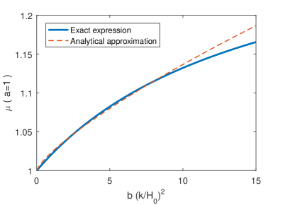
which allows to extract the explicit $b$ and $k/H_{0}$ dependence from the integral in equation (51). We compare in the left panel of Fig. 10 this approximation with the exact expression. We see that it provides an excellent fit for $b(k/H_{0})^{2}<10$. Then, using (51) we get

$$\epsilon(a,k)=\left[b\,\left(\frac{k}{H_{0}}\right)^{2}\right]^{0.77}\,F(a),$$ (61)

being,

$$F(a)=0.8236\,(1-\Omega_{m})^{1.54}\,e^{-g(a)}\,$$

$$\times\int_{a_{i}}^{a}\,\frac{\Omega_{m}^{1-\gamma^{*}}(a^{\prime})}{r^{2.31}(a^{\prime})a^{\prime 2.54}}\,e^{\,g(a^{\prime})}\,da^{\prime}.$$ (62)

The fitting functions for $F(a)$ in terms of $\Omega_{m}(a)$ can be easily obtained and reads

$$F(a)= 0.140\,\Omega_{m}(a)-0.545\,\Omega_{m}^{2}(a)+0.994\,\Omega_{m}^{3}(a)$$

$$-0.905\,\Omega_{m}^{4}(a)+0.315\,\Omega_{m}^{5}(a).$$ (63)

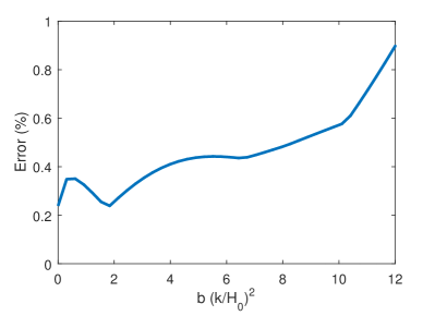
On the right panel of Fig. 10, we plot the growth function errors as a function of $b\,(k/H_{0})^{2}$ using the expressions above. We see that the agreement with the numerical solution is better than $1\%$ when $|\mu-1|<0.12$. Since these fits have been obtained for a $\Lambda$CDM background, using the above expressions with different backgrounds would increase the errors up to $2\%$.

IV.2 Phenomenological parametrization

Let us consider the limit $|\mu_{0}-1|\ll 1$ in the parametrization given in (43). Using equation (51) we find that,

$$\epsilon(a) = \frac{3}{2}\,(\mu_{0}-1)\,\,e^{-g(a)}\,$$ (64)

$$\times \int_{a_{i}}^{a}\,\Omega_{m}^{1-\gamma^{*}}(a^{\prime})\,\frac{1-\Omega_{m}(a^{\prime})}{1-\Omega_{m}}\,\,e^{\,g(a^{\prime})}\,\frac{da^{\prime}}{a^{\prime}},$$

and we can fit this expression as follows,

$$\epsilon(a) = (\mu_{0}-1)\,(0.505-0.646\,\Omega_{m}(a)+0.141\,\Omega_{m}(a)^{2}).$$

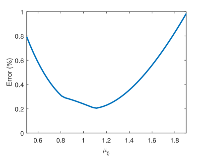
In this case, as we can see in Fig. 11, the error in the growth function is below $1\%$ for $|\mu_{0}-1|<1$. Since, as in the $f(R)$ case, these fits have been obtained for a $\Lambda$CDM background, using the above expressions with different backgrounds would increase the errors up to $2\%$.

Figure 11: Errors in $f(z)$ for the phenomenological parametrization (IV.1) for the $\Lambda$CDM background.

V Fisher matrix and forecasts

The fitting functions for $f$ in terms of the $\mu$ parameter that have been obtained in previous sections can be helpful to asses the capability of future galaxy surveys to constrain modified gravity theories in a model independent way. Let us consider the simplest possibility in which we assume that for the range of redshifts and scales covered by the survey, the $\mu$ factor can be considered as constant. In such a case (22) provides an accurate approximation for the growth function.

The galaxy power spectrum in redshift space, $P(k_{r},\hat{\mu}_{r},z)$ is given by Seo:2003pu

$$P(k_{r},\hat{\mu}_{r},z)=\frac{D_{A\,r}^{2}\,E(z)}{D_{A}^{2}\,E_{r}(z)}\,(b+f\,\hat{\mu}^{2})^{2}\,D^{2}{P}(k)\,e^{-k_{r}^{2}\,\hat{\mu}_{r}^{2}\,\sigma_{r}^{2}},$$ (66)

where, $\hat{\mu}$ is the angle between $\vec{k}$ and the line of sight, $H(z)=H_{0}E(z)$, $D(z)=\delta_{m}(z)/\delta_{m}(0)$ is the growth factor, $b$ is the bias and $f$ is the growth function given by (22) in terms of $\mu$. The sub-index $r$ denotes that the quantity is evaluated for the fiducial model. $\sigma_{r}=\delta z\,(1+z)/H(z)$ with $\delta z(1+z)$ the photometric redshift error and $D_{A}$ is the angular distance, which, in a flat Universe reads $D_{A}(z)=(1+z)^{-1}\,\chi(z)$, where $\chi(z)$ is the comoving radial distance,

$$\chi(z)=H_{0}^{-1}\,\int_{0}^{z}\frac{dz^{\prime}}{E(z^{\prime})},$$ (67)

$P(k)$ is the matter power spectrum which is the output of CAMB Lewis:1999bs using h/Mpc units. Finally, the dependence $k=k(k_{r})$, $\hat{\mu}=\hat{\mu}(\hat{\mu}_{r})$ and the factor $\frac{D^{2}_{Ar}E}{D^{2}_{A}\,E_{r}}$ are due to the Alcock-Paczynski effect Alcock:1979mp ,

$$k=Q\,k_{r},$$ (68)

$$\hat{\mu}=\frac{E\,\hat{\mu}_{r}}{E_{r}\,Q},$$ (69)

$$Q=\frac{\sqrt{E^{2}\,\chi^{2}\,\hat{\mu}^{2}_{r}-E_{r}^{2}\,\chi_{r}^{2}\,(\hat{\mu}^{2}_{r}-1)}}{E_{r}\,\chi}.$$ (70)

We consider a simple model in which we have only two free parameters $\mu$ and $\Omega_{m}$ with a fiducial $\Lambda$CDM cosmology with $\Omega_{c}\,h^{2}=0.121$, $\Omega_{b}\,h^{2}=0.0226$, $\Omega_{\nu}\,h^{2}=0.00064$, $n_{s}=0.96$, $h=0.68$, $H^{-1}_{0}=2997.9\,\textrm{Mpc/h}$, $\Omega_{k}=0$ and $\sigma_{8}=0.82$. In this case

$$E(z)=\sqrt{\Omega_{m}\,(1+z)^{3}+(1-\Omega_{m})}.$$ (71)

For the bias we write $b(z)=\sqrt{1+z}$.

Denoting the free model parameters as $p_{\alpha}=(\Omega_{m},\mu)$ the corresponding Fisher matrix for clustering at a given redshift bin centered at $z$ is Seo:2003pu ,

$$F_{\alpha\beta}=\frac{1}{8\pi^{2}}\int_{-1}^{1}d\hat{\mu}_{r}\int_{k_{\text{min}}}^{k_{max}}k_{r}^{2}\,V_{eff}\,\left.\frac{\partial\ln(P(k_{r},\hat{\mu}_{r},z))}{\partial p_{\alpha}}\right|_{r}\,\left.\frac{\partial\ln(P(k_{r},\hat{\mu}_{r},z))}{\partial p_{\beta}}\right|_{r}\,\,dk_{r},$$ (72)

where $V_{eff}=V_{eff}(k,\hat{\mu},z)|_{r}$ is the effective volume,

$$V_{eff}=\left(\frac{n(z)\,P(k,\hat{\mu},z)}{1+n(z)\,P(k,\hat{\mu},z)}\right)^{2}\,V_{s},$$ (73)

$n(z)$ is the mean galaxy density at redshift $z$ and $V_{s}=\frac{4\pi\,f_{sky}}{3}\,\left(\chi(z_{max})^{3}-\chi(z_{min})^{3}\right)$ is the total volume of the survey where $f_{sky}$ is the sky fraction, $z_{max}$ and $z_{min}$ the maximum and minimum redshifts respectively. $k_{\text{min}}$ is fixed to 0.007 $h$/Mpc and $k_{max}(z=1.3)=0.218\,h/$Mpc Amendola:2013qna . This value of $k_{max}$ corresponds to $\sigma(z,k_{max})=0.35$ so that only linear scales are considered in the calculation.

Notice that thanks to the explicit expression in (22), now it is possible to compute the derivatives with respect to the $\mu$ parameter appearing in the Fisher matrix in a straightforward way.

As an example, we consider and Euclid-like survey Euclid with a unique bin centered at $z=1.3$ with $z_{min}=0.5$, $z_{max}=2.1$, $f_{sky}=0.375$ which correspond to 15500 $\mathrm{deg}^{2}$, $\delta z=0.001$ and $n(z)=1.12\times 10^{-3}$ $(\textrm{h/Mpc})^{3}$.

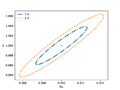
Inverting the Fisher matrix, the marginalized error for the $p_{\alpha}$ parameter is $\sqrt{F^{-1}_{\alpha\alpha}}$. Thus for $\mu$ and $\Omega_{m}$ we find: $\Delta\Omega_{m}=8.76\times 10^{-4}$, $\Delta\mu=0.0026$, which corresponds to $\Delta\Omega_{m}/\Omega_{m}(\%)=0.28\%$, $\Delta\mu/\mu(\%)=0.26\%$. In Fig. 12 we plot the 1-$\sigma$ and 2-$\sigma$ contours for $(\Omega_{m},\mu)$ assuming that the probability distribution function is Gaussian.

Figure 12: 1-$\sigma$ and 2-$\sigma$ contours for $(\Omega_{m},\mu)$ using an example of future galaxy redshift survey with $z$ in $[0.5,2.1]$, 15500 $\mathrm{deg}^{2}$, $\delta z=0.001$ and a mean galaxy density of $n(z)=1.12\cdot 10^{-3}$ $(\textrm{h/Mpc})^{3}$.

VI Discussion of results and conclusions

In this work we aimed at obtaining fitting formulae for the growth function of matter density perturbations in modified gravity theories in a model-independent way. With that purpose, we have considered the $(\mu,\eta)$ parametrization of modified gravities and shown that a generic expression like $f(a)=\beta(a)\Omega_{m}^{\gamma}(a)$ provides good fits to the numerical solutions.

In the time-independent $\mu(k)$ case, explicit expressions for $\beta(\mu)$ and $\gamma(\mu)$ have been obtained for $\Lambda$CDM and modified backgrounds, yielding accuracies better than $0.5\%$.

In the time-dependent but scale-independent $\mu(a)$ case, it is not possible to obtain explicit formulae for $\beta$ and $\gamma$, however, it is shown that a constant $\gamma$ and a $\beta(a)$ function with the same scale factor dependence as $\mu(a)$ provides errors which again can be in the range of $0.5\%$.

Finally, in the general case $\mu(a,k)$, it is possible to obtain explicit generic expressions in the perturbative regime $|1-\mu|\ll 1$. As an example, for the Hu-Sawicki $f(R)$ model, accuracies below $1\%$ are obtained.

The general perturbative expressions derived in this work exhibit explicit dependence both on the wavenumber $k$ and on the model parameters which could be useful in the forecast analysis of modified gravity parameters or in the analysis of growth data of present and future galaxy surveys. A simple Fisher analysis for a future Euclid-like survey has been presented as example. Work is in progress in this direction.

Acknowledgements: We would like to thank M. Quartin for useful comments that motivated this work and Eric V. Linder for helpful comments. M.A.R acknowledges support from UCM predoctoral grant. This work has been supported by the MINECO (Spain) projects FIS2014-52837-P, FIS2016-78859-P(AEI/FEDER, UE), and Consolider-Ingenio MULTIDARK CSD2009-00064.

References

- (1) A. G. Riess et al. [Supernova Search Team Collaboration], Astron. J. 116 (1998) 1009 doi:10.1086/300499 [astro-ph/9805201].
- (2) S. Perlmutter et al. [Supernova Cosmology Project Collaboration], Astrophys. J. 517 (1999) 565 doi:10.1086/307221 [astro-ph/9812133].
- (3) D. J. Eisenstein et al. [SDSS Collaboration], Astrophys. J. 633 (2005) 560 doi:10.1086/466512 [astro-ph/0501171].
- (4) W. J. Percival, S. Cole, D. J. Eisenstein, R. C. Nichol, J. A. Peacock, A. C. Pope and A. S. Szalay, Mon. Not. Roy. Astron. Soc. 381 (2007) 1053 doi:10.1111/j.1365-2966.2007.12268.x [arXiv:0705.3323 [astro-ph]].
- (5) S. Nojiri and S. D. Odintsov, Phys. Rev. D 68 (2003) 123512 doi:10.1103/PhysRevD.68.123512 [hep-th/0307288].
- (6) S. Capozziello, S. Carloni and A. Troisi, Recent Res. Dev. Astron. Astrophys. 1 (2003) 625 [astro-ph/0303041].
- (7) G. R. Dvali, G. Gabadadze and M. Porrati, Phys. Lett. B 485 (2000) 208 doi:10.1016/S0370-2693(00)00669-9 [hep-th/0005016].
- (8) S. Tsujikawa, A. De Felice and J. Alcaniz, JCAP 1301 (2013) 030 doi:10.1088/1475-7516/2013/01/030 [arXiv:1210.4239 [astro-ph.CO]].
- (9) A. Silvestri, L. Pogosian and R. V. Buniy, Phys. Rev. D 87 (2013) no.10, 104015 doi:10.1103/PhysRevD.87.104015 [arXiv:1302.1193 [astro-ph.CO]].
- (10) E. V. Linder, Phys. Rev. D 72 (2005) 043529 doi:10.1103/PhysRevD.72.043529 [astro-ph/0507263].
- (11) E. V. Linder and R. N. Cahn, Astropart. Phys. 28 (2007) 481 doi:10.1016/j.astropartphys.2007.09.003 [astro-ph/0701317].
- (12) N. Benitez et al. [J-PAS Collaboration], arXiv:1403.5237 [astro-ph.CO].
- (13) M. Levi et al. [DESI Collaboration], arXiv:1308.0847 [astro-ph.CO].
- (14) L. Amendola et al. [Euclid Theory Working Group], Living Rev. Rel. 16 (2013) 6 doi:10.12942/lrr-2013-6 [arXiv:1206.1225 [astro-ph.CO]].
- (15) R. Gannouji and D. Polarski, JCAP 0805 (2008) 018 doi:10.1088/1475-7516/2008/05/018 [arXiv:0802.4196 [astro-ph]].
- (16) C. Di Porto and L. Amendola, Phys. Rev. D 77 (2008) 083508 doi:10.1103/PhysRevD.77.083508 [arXiv:0707.2686 [astro-ph]].
- (17) P. A. R. Ade et al. [Planck Collaboration], Astron. Astrophys. 594 (2016) A13 doi:10.1051/0004-6361/201525830 [arXiv:1502.01589 [astro-ph.CO]].
- (18) E. V. Linder, JCAP 1304 (2013) 031 doi:10.1088/1475-7516/2013/04/031 [arXiv:1302.4754 [astro-ph.CO]].
- (19) J. N. Fry, Phys. Lett. 158B (1985) 211. doi:10.1016/0370-2693(85)90957-8
- (20) M. Chevallier and D. Polarski, Int. J. Mod. Phys. D 10 (2001) 213 doi:10.1142/S0218271801000822 [gr-qc/0009008].
- (21) E. V. Linder, Phys. Rev. Lett. 90 (2003) 091301 doi:10.1103/PhysRevLett.90.091301 [astro-ph/0208512].
- (22) J. B. Dent, S. Dutta and L. Perivolaropoulos, Phys. Rev. D 80 (2009) 023514 doi:10.1103/PhysRevD.80.023514 [arXiv:0903.5296 [astro-ph.CO]].
- (23) J. C. Bueno Sanchez, J. B. Dent, S. Dutta and L. Perivolaropoulos, JCAP 1009 (2010) 021 doi:10.1088/1475-7516/2010/09/021 [arXiv:1004.4905 [astro-ph.CO]].
- (24) L. Amendola, M. Kunz and D. Sapone, JCAP 0804 (2008) 013 doi:10.1088/1475-7516/2008/04/013 [arXiv:0704.2421 [astro-ph]].
- (25) M. Ishak and J. Dossett, Phys. Rev. D 80 (2009) 043004 doi:10.1103/PhysRevD.80.043004 [arXiv:0905.2470 [astro-ph.CO]].
- (26) S. Chen and J. Jing, Phys. Lett. B 685 (2010) 185 doi:10.1016/j.physletb.2010.01.061 [arXiv:0908.4379 [gr-qc]].
- (27) Y. Gong, Phys. Rev. D 78 (2008) 123010 doi:10.1103/PhysRevD.78.123010 [arXiv:0808.1316 [astro-ph]].
- (28) F. Simpson et al., Mon. Not. Roy. Astron. Soc. 429 (2013) 2249 doi:10.1093/mnras/sts493 [arXiv:1212.3339 [astro-ph.CO]].
- (29) P. A. R. Ade et al. [Planck Collaboration], Astron. Astrophys. 594 (2016) A14 doi:10.1051/0004-6361/201525814 [arXiv:1502.01590 [astro-ph.CO]].
- (30) A. A. Starobinsky, JETP Lett. 86 (2007) 157 doi:10.1134/S0021364007150027 [arXiv:0706.2041 [astro-ph]].
- (31) W. Hu and I. Sawicki, Phys. Rev. D 76 (2007) 064004 doi:10.1103/PhysRevD.76.064004 [arXiv:0705.1158 [astro-ph]].
- (32) S. A. Appleby and R. A. Battye, Phys. Lett. B 654 (2007) 7 doi:10.1016/j.physletb.2007.08.037 [arXiv:0705.3199 [astro-ph]].
- (33) S. Tsujikawa, Phys. Rev. D 77 (2008) 023507 doi:10.1103/PhysRevD.77.023507 [arXiv:0709.1391 [astro-ph]].
- (34) S. Tsujikawa, R. Gannouji, B. Moraes and D. Polarski, Phys. Rev. D 80 (2009) 084044 doi:10.1103/PhysRevD.80.084044 [arXiv:0908.2669 [astro-ph.CO]].
- (35) R. Gannouji, B. Moraes and D. Polarski, JCAP 0902 (2009) 034 doi:10.1088/1475-7516/2009/02/034 [arXiv:0809.3374 [astro-ph]].
- (36) T. Narikawa and K. Yamamoto, Phys. Rev. D 81 (2010) 043528 Erratum: [Phys. Rev. D 81 (2010) 129903] doi:10.1103/PhysRevD.81.129903, 10.1103/PhysRevD.81.043528 [arXiv:0912.1445 [astro-ph.CO]].
- (37) A. J. López-Revelles, Phys. Rev. D 87 (2013) no.2, 024021 doi:10.1103/PhysRevD.87.024021 [arXiv:1301.2120 [gr-qc]].
- (38) K. Bamba, A. Lopez-Revelles, R. Myrzakulov, S. D. Odintsov and L. Sebastiani, Class. Quant. Grav. 30 (2013) 015008 doi:10.1088/0264-9381/30/1/015008 [arXiv:1207.1009 [gr-qc]].
- (39) H. J. Seo and D. J. Eisenstein, Astrophys. J. 598 (2003) 720 doi:10.1086/379122 [astro-ph/0307460].
- (40) A. Lewis, A. Challinor and A. Lasenby, Astrophys. J. 538 (2000) 473 doi:10.1086/309179 [astro-ph/9911177].
- (41) C. Alcock and B. Paczynski, Nature 281 (1979) 358. doi:10.1038/281358a0
- (42) L. Amendola, S. Fogli, A. Guarnizo, M. Kunz and A. Vollmer, Phys. Rev. D 89 (2014) no.6, 063538 doi:10.1103/PhysRevD.89.063538 [arXiv:1311.4765 [astro-ph.CO]].