Analysis of wavepacket tunneling with the method of Laplace transformation

Abstract

We use the method of Laplace transformation to determine the dynamics of a wave packet that passes a barrier by tunneling. We investigate the transmitted wave packet and find that it can be resolved into a sequence of subsequent wave packages. This result sheds new light on the Hartman effect for the tunneling time and gives a possible explanation for an experimental result obtained by Spielmann et. al.

1 Introduction

There are several definitions of tunneling times ([1],[2],[3],[4],[5],[6],[7],[8]) and the discussion about their meaning is still ongoing ([3],[4],[9],[10]). Recently, experiments with atoms stimulated by ultrashort, infrared laser pulses, the so-called attoclock experiments, reinforced the interest in the prediction of tunneling times ([11],[12],[13]).

In this article we investigate the dynamics of a wavepacket that tunnels through a barrier. The tunneling time we determine is the so-called group delay or phase time ([14],[3]). It can be characterized as the time interval between the moment the peak of a freely evolving incoming wave packet would reach the barrier and the arrival of the peak of the transmitted wave packet at the end of the barrier. One of the oldest results for this tunneling time was obtained by Mac Coll ([15]) in 1932 by the application of the stationary phase method. He concluded that there was ”no appreciable delay in the transmission of the packet through the barrier”. These calculations were later refined by Hartmann ([14],[3]), who found a finite delay time. For thicker barriers this delay time becomes independent of the thickness of the barrier and tends to a fixed value which is known as the Hartmann effect. This saturation was also found for other definitions of tunneling time ([4]), whereas in the framework of fractional quantum mechanics a decreasing of the tunneling time with barrier width was obtained([16]). A formal analogy between the Schrödinger and the Helmholtz equation (see for instance [3])made it possible to test predictions for the tunneling time with optical experiments. The results confirmed the saturation of the tunneling time ([17],[18], [19],see [3] for more references ) though a more detailed discrepancy between experiment and calculations remained open in [18].

Since the Hartmann effect seems to threaten Einstein causality, because superluminal velocities can be infered from transmission times saturating with barrier width , an objection was made that only the modes above the barrier energy may contribute to the transmitted wave packet ([17], [20]). But it was argued in ([21])with reference to numerical calculations and experimental results that this effect can not be used as an explanation of the barrier tunneling phenomenon (see also [3] for a more detailed discussion and further references).

The results of the attoclock experiments with strong laser fields that lower the Coulomb potential can be best explained by using a tunneling time probability amplitude constructed with Feynnman path integrals ([11], [13]), whereas several other definitions of tunneling times do not agree with the data.

At present there exists no unified formalism for the calculation of tunneling times for different experimental settings. In the case of wavepacket tunneling through static barriers the phase time, keeping track of the peak is the best candidate for the tunneling time, and in good agreement with the experimental results([17],[18], [19]).

The phase time is in general obtained by representing the solution of the time-dependent Schrödinger equation as the integral over stationary solutions for different energies. Under the assumption that the energy distribution of the initial wave packet is sufficiently peaked the application of the stationary phase method yields a time for the arrival of the peak of the wavepacket at the end of the barrier.

In this article we use the method of Laplace transformation [22] to determine the wavepacket dynamics.Instead of immediately applying an approximation for oscillatory integrals, we first obtain exact solutions for the wavefunction at each side and inside the barrier, which we then simplify assuming that the initial wavepacket is sufficiently peaked in the momentum representation. Since we are free to choose explicitely the initial wavepacket in position space (which we do not have to construct as superposition of eigenstates), it is technically much easier to start with a wavepacket located exclusively at the left side of the barrier. Furthermore we give estimates for the consequences of the applied approximations and derive a consistency condition in the case of a special class of initial wavepackets.

We find that what comes out of the barrier is not a single wave packet, but infinitely many, one after the other. The time each of these wavepackets needs for the tunneling is completely independent of the thickness of the barrier. But for thicker barriers, the later wavepackets are much more attenuated and so there remains a single transit time that equals the result Hartmann obtained as the upper limit for the tunneling time. However in our approach the tunneling decreases before it reaches the limiting value for thick barriers. This is in accordance with the results of the optical experiments performed by Spielmann et al. [18]. Bernardini ([23]) investigated the transmission of wavepackets with energies above the height of the barrier. He also finds that there is not only one reflected and one transmitted wave packet, but many of them that leave the barrier. This result was obtained by the decomposition of the transmission and reflection coefficients of the stationary solution in infinite series. Our result is the counterpart in the tunneling regime.

2 The solution of the time-dependent Schrödinger equation

A finite barrier is described by the potential

$$\begin{array}[]{lll}V(x)=0&\qquad\mbox{for}&x\,\leq\,0\\ V(x)=V&\qquad\mbox{for}&0\,<x\,<\,d\\ V(x)=0&\qquad\mbox{for}&x\,\geq\,d\quad.\end{array}$$

The dynamics of a wave packet $\psi(x,0)$ is determined by the Schrödinger equation

$$-\frac{\hbar^{2}}{2m}\frac{\partial^{2}\psi(x,t)}{\partial x^{2}}=i\hbar\,\frac{\partial\psi(x,t)}{\partial t}\qquad \mbox{for}\qquad x\,<\,0\,,$$ (1)

$$-\frac{\hbar^{2}}{2m}\frac{\partial^{2}\psi(x,t)}{\partial x^{2}}+V\psi(x,t)=i\hbar\,\frac{\partial\psi(x,t)}{\partial t}\qquad \mbox{for}\qquad 0\,<\,x\,<\,d\,\,,$$ (2)

$$-\frac{\hbar^{2}}{2m}\frac{\partial^{2}\psi(x,t)}{\partial x^{2}}=i\hbar\,\frac{\partial\psi(x,t)}{\partial t}\qquad \mbox{for}\qquad x\,>\,d\,,$$ (3)

where $\psi(x,t)$ is supposed to be continuously differentiable everywhere and square integrable .

We will further assume that the initial wave packets are located at the left side of the barrier

$$\psi(x,0)=0\qquad\mbox{for}\qquad x\geq 0\,.$$ (4)

We apply the method of Laplace transformation, already introduced in ([22]).

The Laplace transformed wavepacket $\varphi(x,s)$

$$\varphi(x,s)=\mathcal{L}(\psi(x,t))=\int\limits_{0}^{\infty}\psi(x,t)e^{-st}dt\quad.$$ (5)

obeys the transformed equations

$$-\frac{\hbar^{2}}{2m}\frac{\partial^{2}\varphi(x,s)}{\partial x^{2}}\,\varphi(x,s)=i\hbar\,s\,\varphi(x,s)-i\hbar\,\psi(x,0)\qquad \mbox{for}\qquad x\,<\,0\,,$$ (6a)

$$-\frac{\hbar^{2}}{2m}\frac{\partial^{2}\varphi(x,s)}{\partial x^{2}}+V\,\varphi(x,s)=i\hbar\,s\,\varphi(x,s)-i\hbar\,\psi(x,0)\qquad \mbox{for}\qquad 0\,<\,x\,<\,d\,\,,$$ (6b)

$$-\frac{\hbar^{2}}{2m}\frac{\partial^{2}\varphi(x,s)}{\partial x^{2}}\,\varphi(x,s)=i\hbar\,s\,\varphi(x,s)-i\hbar\,\psi(x,0)\qquad \mbox{for}\qquad x\,>\,d\,.$$ (6c)

The solution of (6) is determined by the method of variation of constants:

$$\varphi(x,s) =\sqrt{\frac{m}{2is\hbar}}\left\{u_{1}(x,s)\int_{-d}^{x}u_{2}(y,s)\psi(y,0)dy\,-\,\right. \left.u_{2}(x,s)\int_{-d}^{x}u_{1}(y,s)\psi(y,0)dy\right\}$$

$$\quad+\,\alpha(s)u_{1}(x,s)\,+\,\beta(s)u_{2}(x,s) \mbox{for}\quad x\,<\,0\qquad$$ (7a)

$$\varphi(x,s) =\gamma(s)u_{3}(x,s)\,+\,\delta(s)u_{4}(x,s) \mbox{for}\quad 0\,<\,x\,<\,d\qquad$$ (7b)

$$\varphi(x,s) =\mu(s)u_{1}(x,s)\,+\,\nu(s)u_{2}(x,s) \mbox{for}\quad x\,>\,d.\qquad\,$$ (7c)

The functions $u_{1}(x,s),u_{2}(x,s),u_{3}(x,s),u_{4}(x,s)$ are the solutions of the homogeneous equations corresponding to (6)

$$u_{1}(x,s)=e^{i\sqrt{\frac{2msi}{\hbar}}x}\quad u_{2}(x,s)=e^{-i\sqrt{\frac{2msi}{\hbar}}x} \mbox{for}\quad 0\,<\,x\,<\,d$$ (8a)

$$u_{4}(x,s)=e^{-i\sqrt{\frac{2msi}{\hbar}-\frac{2mV}{\hbar^{2}}}x}\, u_{3}(x,s)=e^{i\sqrt{\frac{2msi}{\hbar}-\frac{2mV}{\hbar^{2}}}x} \mbox{for}\quad x\,<\,0,x\,>\,d.$$ (8b)

Since $\varphi(x,s)$ must vanish for $x\rightarrow\pm\infty$, we find

$$\alpha(s)=0\,,\quad\nu(s)=0\,.$$

If we evaluate $\varphi(x,s)$ and its first derivative at $x=0$ and $x=d$, we obtain, imposing continuous differentiability

$$\beta(s)=\sqrt{\frac{m}{2i\hbar s}}\left(I_{1}-I_{2}\right)+\sqrt{\frac{m}{2i\hbar s}}\cdot\frac{2\,I_{2}}{1+\sqrt{1-\frac{V}{i\hbar s}}}\cdot\frac{\rho(s)-e^{-2id\sqrt{\frac{2msi}{\hbar}-\frac{2mV}{\hbar^{2}}}}}{\rho^{2}(s)-e^{-2id\sqrt{\frac{2msi}{\hbar}-\frac{2mV}{\hbar^{2}}}}}$$ (9)

$$\gamma(s)=-\sqrt{\frac{m}{2i\hbar s}}\cdot\frac{2\,I_{2}}{1+\sqrt{1-\frac{V}{i\hbar s}}}\cdot\frac{e^{-2id\sqrt{\frac{2msi}{\hbar}-\frac{2mV}{\hbar^{2}}}}}{\rho^{2}(s)-e^{-2id\sqrt{\frac{2msi}{\hbar}-\frac{2mV}{\hbar^{2}}}}}$$ (10)

$$\delta(s)=\sqrt{\frac{m}{2i\hbar s}}\cdot\frac{2\,I_{2}\,\rho(s)}{1+\sqrt{1-\frac{V}{i\hbar s}}}\cdot\frac{1}{\rho^{2}(s)-e^{-2id\sqrt{\frac{2msi}{\hbar}-\frac{2mV}{\hbar^{2}}}}}\,,$$ (11)

$$\mu(s)=\sqrt{\frac{m}{2i\hbar s}}\cdot\frac{2\,I_{2}}{1+\sqrt{1-\frac{V}{i\hbar s}}}e^{-id\sqrt{\frac{2msi}{\hbar}}}\cdot\frac{1-\rho(s)}{\rho^{2}(s)-e^{-2id\sqrt{\frac{2msi}{\hbar}-\frac{2mV}{\hbar^{2}}}}}e^{-2id\sqrt{\frac{2msi}{\hbar}-\frac{2mV}{\hbar^{2}}}}\,,$$ (12)

where we have introduced the abbreviations

$$I_{1}=\int_{-\infty}^{0}e^{i\sqrt{\frac{2msi}{\hbar}}y}\psi(y,0)dy\,,\quad I_{2}=\int_{-\infty}^{0}e^{-i\sqrt{\frac{2msi}{\hbar}}y}\psi(y,0)dy$$

and also used

$$\rho(s)=\frac{2}{1+\sqrt{1-\frac{V}{\hbar si}}}-1\,.$$ (13)

Inserting this result into (7) and applying the series expansion

$$\frac{1}{1-\rho^{2}(s)e^{2id\sqrt{\frac{2msi}{\hbar}-\frac{2mV}{\hbar^{2}}}}}=\sum_{k=0}^{\infty}(\rho(s))^{2k}e^{2idk\sqrt{\frac{2msi}{\hbar}-\frac{2mV}{\hbar^{2}}}}$$

yields

$$\varphi(x,s)=\sqrt{\frac{m}{2si\hbar}}\left\{\int_{-\infty}^{0}e^{i\sqrt{\frac{2msi}{\hbar}}|x-y|}\psi(y,0)dy+\int_{-\infty}^{0}e^{-i\sqrt{\frac{2msi}{\hbar}}(x+y)}\psi(y,0)dy\cdot\rho(s)\right\}+$$

$$\qquad\sqrt{\frac{m}{2si\hbar}}\sum_{l=0}^{\infty}\int_{-\infty}^{0}e^{2id(l+1)\sqrt{\frac{2msi}{\hbar}-\frac{2mV}{\hbar^{2}}}-i(x+y)\sqrt{\frac{2msi}{\hbar}}}\psi(y,0)dy\cdot(\rho^{2}(s)-1)\rho^{2l+1}(s)$$

$$\qquad\mbox{for}\quad x\,<\,0$$ (14a)

$$\varphi(x,s)=\sqrt{\frac{m}{2si\hbar}}\sum_{l=0}^{\infty}\int_{-\infty}^{0}e^{i(2dl+x)\sqrt{\frac{2msi}{\hbar}-\frac{2mV}{\hbar^{2}}}-iy\sqrt{\frac{2msi}{\hbar}}}\psi(y,0)dy\cdot(\rho(s)+1)\rho^{2l}(s)\,-$$

$$\qquad\sqrt{\frac{m}{2si\hbar}}\sum_{l=0}^{\infty}\int_{-\infty}^{0}e^{i(2d(l+1)-x)\sqrt{\frac{2msi}{\hbar}-\frac{2mV}{\hbar^{2}}}-iy\sqrt{\frac{2msi}{\hbar}}}\psi(y,0)dy\cdot(\rho(s)+1)\rho^{2l+1}(s)\,$$

$$\qquad\mbox{for}\quad 0\,\leq x\,\leq\,d\,,$$ (14b)

$$\varphi(x,s)=\sqrt{\frac{m}{2si\hbar}}\sum_{l=0}^{\infty}\int_{-\infty}^{0}e^{id(2l+1)\sqrt{\frac{2msi}{\hbar}-\frac{2mV}{\hbar^{2}}}+i(x-d-y)\sqrt{\frac{2msi}{\hbar}}}\psi(y,0)dy\cdot(-\rho^{2}(s)+1)\rho^{2l}(s)$$

$$\qquad\mbox{for}\quad x\,>\,d\,.$$ (14c)

We introduce the shifted momentum representation

$$f(Q,p)=\frac{1}{\sqrt{2\pi\hbar}}\int_{-\infty}^{\infty}\psi(x+Q,0)e^{\frac{-ipx}{\hbar}}dx\,=\,e^{\frac{ipQ}{\hbar}}f(p)\,,$$ (15)

where

$$f(0,p)=f(p)$$

denotes the representation of the wave function in momentum space.

Applying the abbreviations

$$a_{l}(t)=\mathcal{L}^{-1}\left\{\rho^{2l+1}(s)(1-\rho^{2}(s))\right\}\,,\quad b_{l}(t)=\mathcal{L}^{-1}\left\{\rho^{2l}(s)(1+\rho(s))\right\}$$

$$c_{l}(t)=\mathcal{L}^{-1}\left\{\rho^{2l+1}(s)(1+\rho(s))\right\}\,,\quad g_{l}(t)=\mathcal{L}^{-1}\left\{\rho^{2l}(s)(1-\rho^{2}(s))\right\}\,,$$

we find proceeding as for the asymmetric square well in [22] for the inverse Laplace transform of (14)

$$\psi(x,t)=\frac{\kappa}{\sqrt{2\pi t\,i}}\int_{-\infty}^{0}e^{\frac{i(x-y)^{2}\kappa^{2}}{2t}}\psi(y,0)dy+\int_{0}^{t}\frac{\kappa}{\sqrt{2\pi(t-\tau)\,i}}\int_{-\infty}^{0}e^{\frac{i(x+y)^{2}\kappa^{2}}{2(t-\tau)}}\psi(y,0)r(\tau)dy\,d\tau\,+$$

$$\quad\sum_{l=0}^{\infty}\int_{0}^{t}\int_{-\infty}^{\infty}K\left(2d(l+1),p,t-\tau\right)f(-x,p)dp\cdot a_{l}(\tau)d\tau$$

$$\quad\mbox{for}\quad x\,<\,0\,,$$ (16a)

$$\psi(x,t)=\sum_{l=0}^{\infty}\int_{0}^{t}\int_{-\infty}^{\infty}K\left(2dl+x),p,t-\tau\right)f(p)dp\cdot b_{l}(\tau)d\tau\,+$$

$$\quad\sum_{l=0}^{\infty}\int_{0}^{t}\int_{-\infty}^{\infty}K\left(d(2l+1)-x),p,t-\tau\right)f(p)dp\cdot c_{l}(\tau)d\tau\,$$

$$\quad\mbox{for}\quad 0\,<\,x\,<\,d\,,$$ (16b)

$$\psi(x,t)=\sum_{l=0}^{\infty}\int_{0}^{t}\int_{-\infty}^{\infty}K\left(d(2l+1),p,t-\tau\right)f(x-d,p)dp\cdot g_{l}(\tau)d\tau\,$$

$$\quad\mbox{for}\quad x\,>\,d\,,$$ (16c)

where $K(x,p,t)$ is defined by

$$K(x,p,t)=\frac{1}{2\sqrt{2\pi\hbar}}e^{\frac{-iVt}{\hbar}-\frac{itq^{2}}{2\hbar m}}\quad\cdotp$$

$$\quad\left\{e^{-\frac{ixq}{\hbar}}\mbox{Erfc}\left[-i\sqrt{\frac{2mi}{\hbar\,t}}\frac{x}{2}-i\sqrt{\frac{i\,t}{2\hbar m}}q\right]+e^{\frac{ixq}{\hbar}}\mbox{Erfc}\left[-i\sqrt{\frac{2mi}{\hbar\,t}}\frac{x}{2}+i\sqrt{\frac{i\,t}{2\hbar m}}q\right]\right\}\,,$$

and we used $\kappa=\sqrt{\frac{m}{\hbar}}$ and $q=\sqrt{p^{2}-2mV}$.

3 Tunneling of wave packets

In order to investigate the tunneling process, we consider a wave packet that is represented in momentum space by

$$f(p)=e^{\frac{-ipx_{0}}{\hbar}}F\left(p-p_{0}\right)\quad,$$ (18a)

where $F(p)$ fulfills

$$\int_{-\infty}^{\infty}F^{*}(p)\,p\,F(p)dp=0\,,\qquad\int_{-\infty}^{\infty}\,F^{*}(p)F^{\prime}(p)dp=0\,.$$ (18b)

. The expectation values of position and momentum are then given by

$$\left\langle\hat{x}\right\rangle=x_{0}\,,\qquad\left\langle\hat{p}\right\rangle=p_{0}\,.$$

We assume that the wavepacket is concentrated within a region $0\,<\,p\,<p_{max}\,<\sqrt{2mV}$. so that we can use the approximation

$$f(p)\approx 0\quad\mbox{for}\quad p\,>\,p_{max}\quad\mbox{and}\quad p\,<\,p_{min}\,.$$ (19)

Moreover it should be sufficiently peaked around the momentum expectation value to justify the approximation

$$F(p-p_{0})(p-p_{0})\approx 0\,.$$ (20)

Finally the difference $\sqrt{2mV}-p_{m}$ should be big enough to ensure

$$\frac{1}{\sqrt{1-\frac{p^{2}}{2mV}}}=O(1)\quad\mbox{for}\quad p_{min}\,\leq\,p\,\leq\,p_{max}\,.$$ (21)

In Appendix B it is shown that these assumptions about the momentum distribution are compatible with the requirement (4) for $\psi(x,0)$.

We start with the solution for $x>d$ (14c). If we rewrite $K(x,p,t)$ for $q^{2}=p^{2}-2mV\,<\,0$ and use

$$X_{l}\equiv d(2l+1)\,,$$

we find (see section 4.4 in [22] for details)

$$K(X_{l},p,t)=U_{0}+U_{1}-U_{2}\,,\quad\mbox{where}\quad$$ (22)

$$U_{0}=e^{-\frac{iVt}{\hbar}}\frac{1}{\sqrt{2\pi\hbar}}e^{-\frac{itq^{2}}{2\hbar m}+\frac{iX_{l}q}{\hbar}}=\frac{1}{\sqrt{2\pi\hbar}}e^{-\frac{ip^{2}t}{2m\hbar}-\frac{X_{l}\sqrt{2mV-p^{2}}}{\hbar}}\,,$$

$$U_{1}=\frac{\kappa}{\sqrt{2\pi t\,i}}\frac{1}{\sqrt{2\pi\hbar}}e^{-\frac{iVt}{\hbar}}\int_{0}^{\infty}e^{\frac{i(X_{l}+u)^{2}\kappa^{2}}{2t}}e^{\frac{i\sqrt{2mV-p^{2}}u}{\hbar}}du\,,$$ (23)

$$U_{2}=\frac{\kappa}{\sqrt{2\pi t\,i}}\frac{1}{\sqrt{2\pi\hbar}}e^{-\frac{iVt}{\hbar}}\int_{0}^{\infty}e^{\frac{i(X_{l}-u)^{2}\kappa^{2}}{2t}}e^{\frac{i\sqrt{2mV-p^{2}}u}{\hbar}}du\,.$$

Inserting

$$\frac{\kappa}{\sqrt{2\pi t\,i}}e^{\frac{i(X_{l}\pm u)^{2}\kappa^{2}}{2t}}=\int_{-\infty}^{\infty}\frac{1}{2\pi\hbar}e^{\frac{-iq^{2}t}{2m\hbar}+\frac{iqX_{l}}{\hbar}\pm\frac{iqu}{\hbar}}dq\,,$$

we obtain

$$U_{1}-U_{2}=\frac{1}{(2\pi\hbar)^{3/2}}e^{-\frac{iVt}{\hbar}}\int_{-\infty}^{\infty}e^{\frac{-iq^{2}t}{2m\hbar}+\frac{iqX_{l}}{\hbar}}\frac{2i\hbar q}{2mV-p^{2}+q^{2}}dq\,.$$ (24)

We find for $U_{1}-U_{2}$, that contains no oscillatory part

$$\int_{-\infty}^{\infty}(U_{1}-U_{2})f(x-d,p)dp\approx 0\,,$$ (25)

since

$$\int_{-\infty}^{\infty}f(p)p^{n}e^{i\frac{p(x-d)}{\hbar}}dp=\left(-i\hbar\frac{\partial}{\partial x}\right)^{n}\psi(x-d,0)=0\quad\mbox{for}\quad\,x\,>\,d\,,\,n=0,1,2,N\,,$$

and so the contribution to (25) will be proportional to $\Delta p^{N+1}$ , if $f(p)$ decays rapidly enough so that the integrals

$$\int_{-\infty}^{\infty}f(p)p^{n}dp$$

exist up to $n=N+1$.

If $\psi(x)$ is infinitely differentiable for $x>d$, th eleft hand side of (25) vanishes identically. So we conclude that for wavepackets that are sufficiently smooth for $x\,>\,d$ , $U_{0}$ is the only relevant contribution.

We obtain for the wavefunction for $x\,>\,d$

$$\psi(x,t)\approx\sum_{l=0}^{\infty}\int_{0}^{t}\frac{1}{\sqrt{2\pi\hbar}}e^{-\frac{X_{l}\sqrt{2mV-p_{0}^{2}}}{\hbar}}\int_{-\infty}^{\infty}e^{-\frac{ip^{2}(t-\tau)}{2m\hbar}}e^{\frac{ip(x-d)}{\hbar}}f(p)dp\cdot g_{l}(\tau)d\tau\,.$$ (26)

This result contains the free time evolution of the initial wave packet that is shifted by $d$ to the right. Proceeding as for the asymmetric square well(see [22]) we can approximate the convolution integral by

$$\int_{0}^{t}\frac{1}{\sqrt{2\pi\hbar}}\int_{-\infty}^{\infty}e^{-\frac{ip^{2}(t-\tau)}{2m\hbar}}e^{\frac{ip(x-d)}{\hbar}}f(p)dp\cdot g_{l}(\tau)d\tau\approx$$ (27)

$$\int_{0}^{\infty}\frac{1}{\sqrt{2\pi\hbar}}\int_{-\infty}^{\infty}e^{-\frac{ip^{2}(t-\tau)}{2m\hbar}}e^{\frac{ip(x-d)}{\hbar}}f(p)dp\cdot g_{l}(\tau)d\tau\approx$$

$$\frac{1}{\sqrt{2\pi\hbar}}\int_{-\infty}^{\infty}e^{-\frac{ip^{2}t}{2m\hbar}}e^{\frac{ip(x-d)}{\hbar}}R(p)^{2l}(1-R(p)^{2})f(p)dp\,$$ (28)

$$\approx R(p_{0})^{2l}(1-R(p_{0})^{2})\cdot\frac{1}{\sqrt{2\pi\hbar}}\int_{-\infty}^{\infty}e^{-\frac{ip^{2}t}{2m\hbar}}e^{\frac{ip(x-d)}{\hbar}}f(p)dp\,,$$ (29)

where $R(p)$ is given by

$$R(p)=-1+2k-2\sqrt{k(k-1)}\quad\mbox{with}\quad k=\frac{p^{2}}{2mV}\,.$$ (30)

Here the assumptions about the concentration of the wave packet (20, 21) justifies putting $R(p)$ before the integral. Evaluating the sum in (26), we obtain

$$\psi(x,t)\approx\sum_{l=0}^{\infty}\int_{0}^{t}\frac{1}{\sqrt{2\pi\hbar}}e^{-\frac{X_{l}\sqrt{2mV-p_{0}^{2}}}{\hbar}}\int_{-\infty}^{\infty}e^{-\frac{ip^{2}(t-\tau)}{2m\hbar}}e^{\frac{ip(x-d)}{\hbar}}f(p)dp\cdot g_{l}(\tau)d\tau\approx$$

$$\frac{e^{\frac{-d\sqrt{2mV-p_{0}^{2}}}{\hbar}}}{1-e^{\frac{-2d\sqrt{2mV-p_{0}^{2}}}{\hbar}}R^{2}(p_{0})}(1-R^{2}(p_{0}))\frac{1}{\sqrt{2\pi\hbar}}\int_{-\infty}^{\infty}e^{-\frac{ip^{2}t}{2m\hbar}}e^{\frac{ip(x-d)}{\hbar}}f(p)dp\,.$$ (31)

For the neglected part of the time integral (27)

$$\Delta_{l}\equiv\int_{t}^{\infty}\frac{1}{\sqrt{2\pi\hbar}}\int_{-\infty}^{\infty}e^{-\frac{ip^{2}(t-\tau)}{2m\hbar}}e^{\frac{ip(x-d)}{\hbar}}f(p)dp\cdot g_{l}(\tau)d\tau\,,$$ (32)

we find the estimates (see Appendix A)

$$\left|\Delta_{l}\right|\sim O(l)\cdot O\left(\left[\frac{2\hbar}{Vt}\right]^{\frac{1}{4}}\right)$$ (33)

Since

$$\sum_{l=0}^{\infty}e^{-\frac{X_{l}\sqrt{2mV-p_{0}^{2}}}{\hbar}}\Delta_{l}\sim\frac{e^{\frac{d\sqrt{2mV-p_{0}^{2}}}{\hbar}}}{\left(-1+e^{\frac{2d\sqrt{2mV-p_{0}^{2}}}{\hbar}}\right)^{2}}\cdot O\left(\left[\frac{2\hbar}{Vt}\right]^{\frac{1}{4}}\right)$$

the approximation for $\psi(x,t)$ given by (3) can be used for $t\gg\frac{\hbar}{V}$.

The wavepacket 3 describes a free evolving wavepacket that started at $t=0$ at the position $x_{0}+d$. It leaves the barrier without any time delay and is instantaneously transmitted through the barrier attenuated by a factor of the magnitude

$$e^{\frac{-d\sqrt{2mV-p_{0}^{2}}}{\hbar}}\,.$$ (34)

So within our approximations we find that the tunneling time is zero, where we assume in accordance with [14] that the transmission begins when a freely evolving wave packet starting at $t=0$ at the position $x_{0}$ would have arrived at the barrier, or equivalently when a classical particle starting at $t=0,x_{0}=0$ has reached the barrier. It is not practicable to follow the peak of the original wavepacket until the entrance of the tunnel since this peak will be deformed by oscillations during the reflection process([22],[25]) and also the position expectation value might undergo a slight attenuation before the tunnel as it was shown for infinite walls ([26]).

Performing the inverse Laplace transform for $x<0$ and $0\,<\,x\,<\,d$ (14a,14a)and making the same approximations as in the previous case we find for the wavepacket to the left of and within the barrier:

$$\psi(x,t)\approx\frac{\kappa}{\sqrt{2\pi t\,i}}\int_{-\infty}^{0}e^{\frac{i(x-y)^{2}\kappa^{2}}{2t}}\psi(y,0)dy+\frac{1}{\sqrt{2\pi\hbar}}\int_{-\infty}^{\infty}e^{-\frac{ip^{2}t}{2m\hbar}}e^{\frac{-ipx}{\hbar}}R(p)f(p)dp+$$

$$\sum_{l=0}^{\infty}e^{-\frac{2d(l+1)\sqrt{2mV-p_{0}^{2}}}{\hbar}}\frac{1}{\sqrt{2\pi\hbar}}\int_{-\infty}^{\infty}e^{-\frac{ip^{2}t}{2m\hbar}}e^{\frac{-ipx}{\hbar}}R(p)^{2l+1}(R(p)^{2}-1)f(p)dp\approx$$

$$\frac{\kappa}{\sqrt{2\pi t\,i}}\int_{-\infty}^{0}e^{\frac{i(x-y)^{2}\kappa^{2}}{2t}}\psi(y,0)dy+$$

$$\left\{1+\frac{e^{\frac{-2d\sqrt{2mV-p_{0}^{2}}}{\hbar}}}{1-e^{\frac{-2d\sqrt{2mV-p_{0}^{2}}}{\hbar}}R(p_{0})^{2}}\cdot(R^{2}(p_{0})-1)\right\}R(p_{0})\frac{1}{\sqrt{2\pi\hbar}}\int_{-\infty}^{\infty}e^{-\frac{ip^{2}t}{2m\hbar}}e^{\frac{-ipx}{\hbar}}f(p)dp$$

$$\mbox{for}\,x\,<\,0\,,$$ (35)

$$\psi(x,t)\approx\sum_{l=0}^{\infty}e^{-\frac{(2dl+x)\sqrt{2mV-p_{0}^{2}}}{\hbar}}\frac{1}{\sqrt{2\pi\hbar}}\int_{-\infty}^{\infty}e^{-\frac{ip^{2}t}{2m\hbar}}R(p)^{2l}(R(p)+1)f(p)dp\approx$$

$$\,-\sum_{l=0}^{\infty}e^{-\frac{(2d(l+1)+x)\sqrt{2mV-p_{0}^{2}}}{\hbar}}\frac{1}{\sqrt{2\pi\hbar}}\int_{-\infty}^{\infty}e^{-\frac{ip^{2}t}{2m\hbar}}R(p)^{2l+1}(R(p)+1)f(p)dp\approx$$

$$\left\{\frac{1}{1-e^{\frac{-2d\sqrt{2mV-p_{0}^{2}}}{\hbar}}R(p_{0})^{2}}\,-\,\frac{e^{\frac{-2(d-x)\sqrt{2mV-p_{0}^{2}}}{\hbar}}}{1-e^{\frac{-2d\sqrt{2mV-p_{0}^{2}}}{\hbar}}R(p_{0})^{2}}\cdot R(p_{0})\right\}$$

$$\,\cdot(R(p_{0})+1)e^{\frac{-x\sqrt{2mV-p_{0}^{2}}}{\hbar}}\cdot\,\frac{1}{\sqrt{2\pi\hbar}}\int_{-\infty}^{\infty}e^{-\frac{ip^{2}t}{2m\hbar}}f(p)dp$$

$$\mbox{for}\,0\,<\,x\,<\,d\,.$$ (36)

The solution within the barrier differs from the solution of the potential step (see [22]) only by a time-independent factor

$$\psi_{step}(x,t)\approx(1+R(p_{0}))e^{-\frac{\sqrt{2mV-p_{0}^{2}}x}{\hbar}}\frac{1}{\sqrt{2\pi\hbar}}\int_{-\infty}^{\infty}e^{\frac{-ip^{2}t}{2m\hbar}}f(p)dp\,.$$ (37)

So we see that the time it needs until the barrier is (approximately) empty again, is independent of the thickness of the barrier. The solution on the left side consists of the incoming and the reflected wave packet (35). In contrast to the potential step the reflected wavepacket experiences a permanent attenuation, since a part of the wavefunction has tunneled through the barrier. After the reflection process the wavefunction consists of a reflected and a transmitted wavepacket (3) only. An explicit calculation yields

$$\left|\left\{1+\frac{e^{\frac{-2d\sqrt{2mV-p_{0}^{2}}}{\hbar}}}{1-e^{\frac{-2d\sqrt{2mV-p_{0}^{2}}}{\hbar}}R(p_{0})^{2}}\cdot(R^{2}(p_{0})-1)\right\}R(p_{0})\right|^{2}+$$ (38)

$$\left|\frac{e^{\frac{-d\sqrt{2mV-p_{0}^{2}}}{\hbar}}}{1-e^{\frac{-2d\sqrt{2mV-p_{0}^{2}}}{\hbar}}R^{2}(p_{0})}(1-R^{2}(p_{0}))\right|^{2}\,=\,1\,,$$ (39)

which confirms that the integral over the probability density is conserved and our approximations are consistent.

4 The tunneling time

Within our approximations we found the tunneling time to be zero, since our solution (3) indicates that the wavepacket leaves the tunnel, shifted by d to the right. Here we have assumed, that all functions of $R(p)$ can be pulled out of the integral (28), and therefore they do not influence the dynamics of the wave packet. If we take into account the first order contributions of $R(p)$, we find a small, but finite tunneling time. We will from now on assume that the initial wave function is an uncorrelated function of the form

$$f(p)=G(p)e^{\frac{-ipx_{0}}{\hbar}}\,,$$

where $G(p)$ is a real function that yields a momentum expectation value $p_{0}$. The position expectation value is then given by $x_{0}$.

The impact of an additional factor $Z(p)$ on the initial wavepacket $f(p)$ is twofold

$$Z(p)f(p)=z(p)e^{i\mu(p)}f(p)\,,\mbox{where}\quad z(p)=|Z(p)|\,.$$ (40)

The probability density in momentum space is only affected by the absolute value $z(p)$. If we restrict ourselves to first order contributions in $p-p_{0}$,

$$z(p)\approx z(p_{0})+z_{1}(p-p_{0})$$

we find that we can neglect the momentum shift:

$$N^{2}\equiv\int_{-\infty}^{\infty}|f(p)|^{2}z(p)^{2}dp\approx z(p_{0})^{2}\int_{-\infty}^{\infty}|f(p)|^{2}dp\,=z(p_{0})^{2}$$ (41)

$$\left\langle\hat{p}\right\rangle\,=\,N^{-2}\int_{-\infty}^{\infty}p|f(p)|^{2}z(p)^{2}dp$$ (42)

$$\approx p_{0}+2(z(p_{0}))^{-1}z_{1}\int_{-\infty}^{\infty}|f(p)|^{2}p(p-p_{0})dp\approx p_{0}\,.$$ (43)

Using also a linear approximation for $\mu^{\prime}(p)$

$$\mu^{\prime}(p)\approx\mu_{1}+\mu_{2}(p-p_{0})\,$$

we find for the position expectation value

$$\widetilde{x_{0}}=N^{-2}\int_{-\infty}^{\infty}z(p)f^{*}(p)e^{-i\mu(p)}\left(i\hbar\frac{\partial}{\partial p}\right)z(p)f(p)e^{i\mu(p)}dp=$$ (44)

$$N^{-2}x_{0}\int_{-\infty}^{\infty}G(p)^{2}z(p)^{2}dp-N^{-2}\hbar\int_{-\infty}^{\infty}G(p)^{2}z(p)^{2}\mu^{\prime}(p)dp$$ (45)

$$\approx x_{0}-\hbar\mu_{1}\,.$$ (46)

Therefore the phase of the functions

$$R(p)^{2l}(1-R(p)^{2})$$ (47)

in (28) yields a shift of the position of each particular wave packet constituting (3)

$$\psi(x,t)\approx\sum_{l=0}^{\infty}\frac{1}{\sqrt{2\pi\hbar}}e^{-\frac{X_{l}\sqrt{2mV-p_{0}^{2}}}{\hbar}}\int_{-\infty}^{\infty}e^{-\frac{ip^{2}t}{2m\hbar}}e^{\frac{ip(x-d)}{\hbar}}R(p)^{2l}(1-R(p)^{2})f(p)dp\,.$$ (48)

We find

$$Arg\left[1-R(p)^{2}\right]=Arctan\left[\frac{-1+2l}{2\sqrt{k-k^{2}}}\right]\approx Arctan\left[\frac{-1+2k_{0}}{2\sqrt{k_{0}-k_{0}^{2}}}\right]+\frac{2}{\sqrt{2mV-p^{2}_{0}}}\cdot(p-p_{0})$$ (49)

$$Arg\left[R(p)\right]=-Arccos\left[1-2k\right]\approx-Arccos\left[1-2k_{0}\right]+\frac{2}{\sqrt{2mV-p^{2}_{0}}}\cdot(p-p_{0})\,,$$ (50)

where we have used the definitions

$$k=\frac{p^{2}}{2mV}\,,\quad k_{0}=\frac{p_{0}^{2}}{2mV}\,.$$

So we see that the lth term of (3) will experience a phase shift of

$$\frac{2(1+2l)(p-p_{0})}{\sqrt{2mV-p^{2}_{0}}}\,,$$

corresponding to a translation by

$$\delta x_{l}=\frac{2(1+2l)\hbar}{\sqrt{2mV-p^{2}_{0}}}=\frac{2(1+2l)\hbar}{p_{0}}\sqrt{\frac{k_{0}}{1-k_{0}}}$$ (51)

to the left. So the delay time will be

$$T_{l}=\frac{2(1+2l)m\hbar}{p_{0}\sqrt{2mV-p^{2}_{0}}}$$

instead of zero.

Each term is attenuated by a factor of the magnitude

$$e^{\frac{-X_{l}\sqrt{2mV-p_{0}^{2}}}{\hbar}}\,.$$ (52)

For thick barriers, if

$$d\frac{\sqrt{2mV-p_{0}^{2}}}{\hbar}\gg 1\,,$$

the first term will dominate the sum (3), and the tunneling time will be given by

$$T_{0}=\frac{2m\hbar}{\sqrt{2mV-p^{2}_{0}}p_{0}}$$ (53)

This is exact the time Hartmann [14]found as upper limit for the tunneling time through thick barriers. If the barrier gets thinner the other wavepackets for $l>0$ will also come into play (see figure 1). Each of them leaves the barrier at a different time $T_{l}$. But since they appear very shortly after each other they may appear as one smeared out wavepacket with a delay time bigger than $T_{0}$.

Note that apart from the absolute and relative magnitude of the wavepackets, all characteristic quantities of tunneling are independent of the width $d$. In the case of the wavefunction pictured in figure 1 where the uncertainties are given by

$$\Delta x\approx\sqrt{\frac{a}{2}}\,,\quad\Delta p\approx\sqrt{\frac{\hbar}{2a}}\,,$$ (54)

the ratio between the distance of the centre of the wavepackets and the position uncertainty the determines the distinguishability between the wavepackets reads

$$\frac{\delta x_{l+1}-\delta x_{l}}{\Delta x}=\frac{4\hbar}{p_{0}\Delta x}\sqrt{\frac{k_{0}}{1-k_{0}}}\approx\frac{8\Delta p}{p_{0}}\sqrt{\frac{k_{0}}{1-k_{0}}}\,.$$ (55)

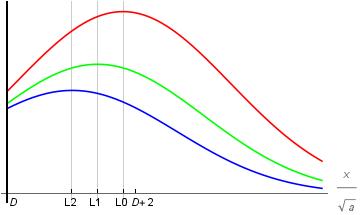
Figure 1: The relative dimensionless probability density $|\psi|^{2}\cdot(\pi a)^{1/2}$ of the first three wavepackets leaving a barrier with the width $d=D\cdot\sqrt{a}$. The initial wavepacket is of the form (64) with the choice of parameters $x_{0}=-20\cdot\sqrt{a}$, $p_{0}=10\cdot\hbar/\sqrt{a}$, $L=20,\,k_{0}=1/2$, where $L$ characterizes the detailed decreasing behaviour. The uncertainties are determined by (65):$(\Delta x)^{2}=0.49\cdot a$, $(\Delta p)^{2}=0.51\cdot\hbar^{2}\cdot a^{-1}$. The first three terms of (48) were evaluated at the time $t=t_{R}+2\cdot\sqrt{a}\cdot m\cdot p_{0}^{-1}$ where $t_{R}=-x_{0}\cdot m\cdot p_{0}^{-1}$ denotes the time when the centre of a freely evolving wavepacket starting at $x_{0}$ has reached the barrier. An instantaneously transmitted wavepacket would then immediately be at position $D\cdot\sqrt{a}$ and therefore reach $\sqrt{a}\cdot(D+2)$ after a time interval $2\sqrt{a}\cdot m\cdot p_{0}^{-1}$. The evaluation shows a slight delay according to (51), so that the wavepackets are centred at $L0\cdot\sqrt{a}=D\cdot\sqrt{a}-2\cdot\hbar\cdot p_{0}^{-1}$, $L1\cdot\sqrt{a}=D\cdot\sqrt{a}-6\cdot\hbar\cdot p_{0}^{-1}$, $L2\cdot\sqrt{a}=D\cdot\sqrt{a}-10\cdot\hbar\cdot p_{0}^{-1}$. Note that the width $d$ only matters with regard to the magnitude of the wavepackets and apart from this the picture applies to a range of possible widths restricted only by the consistency condition (74). Here we have chosen the magnitude of the wavepackets arbitrarily to provide a better visibility. The integrals were numerically evaluated with Wolfram Mathematica, so that the picture is an additional confirmation of (51). Due to the high concordance of the wavefunction with its extension along the real line we could use this extended function for the calculations (see Appendix B).

5 Discussion and conclusions

Our result for the tunneling time (53) is not an exact reproduction of Hartmann’s result ([14],[3]) which predicts an increasing tunneling time with the thickness of the barrier before saturation takes place. However Spielmann et al. found a decreasing tunneling time in their experiments with electromagnetic waves propagating through photonic band gap materials (see [18] fig. 3, [24] fig 1 ). This qualitative behaviour is in good agreement with our results that also predict a decreasing tunneling time since for thicker barriers the later wave packets are more and more attenuated.

For thicker barriers the conclusion of both calculations is that the tunneling time for sufficiently peaked wave packets is given by (53). This is as far interesting as the results were obtained by completely different methods. Moreover we ensured in our calculations that the initial wavepacket is only located at the left side of the barrier (4) which is not clearly guaranteed by Hartmann’s approach. So our result makes sure that the Hartmann time (53) is not some relic of the parts of the initial wavepacket that were at the right hand side of the barrier from the beginning.

We did not take into account the parts of the initial wavepacket with energies near or greater than the critical energy of standard transmission through the barrier (see 19). In Appendix B we have derived a consistency condition for this approximation for the case of a special class of initial wavepackets. So this is a further counterexample to the idea that only energies greater than the barrier height contribute to tunneling ([20]).

We also found out that the approximate solution within a finite barrier differs from the solution within the potential step only by a time-independent factor (36,37) which also indicates that important dynamical properties are independent of the thickness of the barrier. It would be especially interesting if this is also true for more general tunneling processes as the tunneling out of a potential well that could model radioactive decay or tunneling out of atoms as provided by the attoclock experiment [7]. Moreover an application of the method of Laplace transformation to relativistic wave equations would yield a picture of the reflection and tunneling processes in the relativistic case.

Appendix A Estimation of the convolution integral

According to [27], the inverse Laplace transform of $\rho(s)^{l}$ is given by

$$\mathcal{L}^{-1}\left(\rho(s)^{l}\right)=\frac{l}{i^{l}t}J_{l}\left[\frac{Vt}{2\hbar}\right]e^{-\frac{iVt}{2\hbar}}\,.$$ (56)

Therefore we find

$$g_{l}(t)=\mathcal{L}^{-1}\left(\rho^{(}2l)(s)(1-\rho^{2}(s))\right)=\frac{l}{i^{(}2l)t}J_{2l}\left[\frac{Vt}{2\hbar}\right]e^{-\frac{iVt}{2\hbar}}-\frac{l}{i^{(}2(l+1))t}J_{2(l+1)}\left[\frac{Vt}{2\hbar}\right]e^{-\frac{iVt}{2\hbar}}\,.$$ (57)

For an integral of the form

$$u(l,t)=\int_{t}^{\infty}e^{\frac{\mp ipQ}{\hbar}}e^{-\frac{ip^{2}(t-\tau)}{2m\hbar}}e^{-\frac{iV\tau}{2\hbar}}\frac{l}{i^{l}\,\tau}J_{l}\left[\frac{V\tau}{2\hbar}\right]d\tau\,,$$ (58)

we get the following estimate

$$\left|u(l,t)\right|=\left|\int_{t}^{\infty}e^{\frac{ip^{2}\tau}{2m\hbar}-\frac{iV\tau}{2\hbar}}\frac{l}{\tau}J_{l}\left[\frac{Vt}{2\hbar}\right]d\tau\right|\,\leq\int_{\frac{tV}{2\hbar}}^{\infty}\left|\frac{l\,J_{l}(y)}{y}\right|dy\,\leq$$ (59a)

$$\left(\int_{\frac{tV}{2\hbar}}^{\infty}\frac{l}{y^{1+2\epsilon}}dy\right)^{\frac{1}{2}}\cdot\left(\int_{0}^{\infty}\frac{\left(J_{l}(y)\right)^{2}}{y^{1-2\epsilon}}\right)^{\frac{1}{2}}\,=\,$$ (59b)

$$l\frac{1}{\sqrt{2\epsilon}}\left(\frac{2\hbar}{Vt}\right)^{\epsilon}\cdot\left(2^{2\epsilon}\frac{\Gamma[1-2\epsilon]\Gamma[l+\epsilon]}{2(\Gamma[1-\epsilon])^{2}\Gamma[1+l-\epsilon]}\right)^{\frac{1}{2}}\,\leq$$ (59c)

$$l\frac{1}{\sqrt{2\epsilon}}\left(\frac{2\hbar}{Vt}\right)^{\epsilon}\cdot\left(2^{2\epsilon}\frac{\Gamma[1-2\epsilon]}{2(\Gamma[1-\epsilon])^{2}}\right)^{\frac{1}{2}}\quad\mbox{with}\quad 0\,<\,\epsilon\,<\,\frac{1}{2}\,,$$ (59d)

where we have applied the Schwarz inequality and the integral formula ([28])

$$\int_{0}^{\infty}\frac{\left(J_{l}(y)\right)^{2}}{y^{1-2\epsilon}}=2^{2\epsilon}\frac{\Gamma[1-2\epsilon]\Gamma[l+\epsilon]}{2(\Gamma[1-\epsilon])^{2}\Gamma[1+l-\epsilon]}\,.$$ (60)

So we conclude setting $\epsilon=1/4$ for $\Delta_{l}$ (32)

$$\left|\Delta_{l}\right|\sim O(l)\cdot O\left(\left[\frac{2\hbar}{Vt}\right]^{\frac{1}{4}}\right)$$ (61)

Appendix B Decreasing behaviour in momentum space of functions with compact support and the examination of the used assumptions about orders of magnitude based on an example

According to the Palay Wiener theorem ([29]), functions with compact support in position space can not be restricted to a finite interval in momentum space as well. Nevertheless the concentration of those functions in momentum space around their expectation value can be shown to be prescribed by the Fourier transform of a generic reference function. We choose an appropriate wavepacket with a reference function of Gaussian shape and derive the conditions that justify (19,20,21). We also show that we can use the reference function for the evaluation of (48) as we did for the example presented in figure 1.

We start with a normalized wavefuntion $\psi(x)$ with position expectation value $x_{0}$ that is assumed to be zero for $|x-x_{0}|\,\geq\,B$. Let $\psi_{0}(x)$ be a generic reference function that fulfills

$$\begin{array}[]{lll}\psi_{0}(x)=\psi(x)&\qquad\mbox{for}&|x-x_{0}|\,\leq\,B\\ \psi_{0}(x)=-\delta\psi(x)&\qquad\mbox{for}&|x-x_{0}|\,>\,B\quad,\end{array}$$

where $\delta\psi$ is zero for $|x-x_{0}|\,\leq\,B$. Then $\psi(x)$ is represented by the sum

$$\psi(x)=\psi_{0}(x)+\delta\psi(x)$$ (62)

If the norm of $\delta\psi$ is given by $\epsilon$ we find for the reference function

$$\langle\psi_{0}|\psi_{0}\rangle\,=1+\epsilon^{2}\,.$$

The representation of $\psi(x)$ in momentum space reads

$$f(p)=f_{0}(p)+\delta f(p)$$

where $f_{0}(p)$ and $\delta f(p)$ are the representations $\psi_{0}(x)$ and $\delta\psi(x)$ in momentum space.

Using the Schwarz inequality and taking into account that the Fourier transform preserves the $L_{2}$ norm we get for the integral over the momentum density in the region outside the interval $(p_{min},p_{max})$

$$\int_{-\infty}^{p_{min}}f^{*}(p)f(p)\,dp+\int_{p_{max}}^{\infty}f^{*}(p)f(p)\,dp\,\leq$$ (63)

$$\int_{-\infty}^{p_{min}}f_{0}^{*}(p)f_{0}(p)\,dp+\int_{p_{max}}^{\infty}f_{0}^{*}(p)f_{0}(p)dp\,+\epsilon^{2}+2\sqrt{1+\epsilon^{2}}\epsilon\,.$$

In order to provide an explicit example, we choose the initial wavepacket with the position and momentum expectation values $x_{0},p_{0}$

$$\psi(x)=N^{-1/2}e^{-\frac{ip_{0}x}{\hbar}}e^{-\frac{(x-x_{0})^{2}}{2a}}\left[-L+\frac{x-x_{0}}{\sqrt{a}}\right]^{2}\left[L+\frac{x-x_{0}}{\sqrt{a}}\right]^{2}\quad \mbox{for}\quad|x-x_{0}|\,<\,L\sqrt{a}$$ (64a)

$$\psi(x)=0\quad \mbox{for}\quad|x-x_{0}|\,\geq\,L\sqrt{a}\,,$$ (64b)

where the normalization constant $N$ is given by

$$N=\frac{\sqrt{a}}{16}e^{-L^{2}}(2L(-105+50L^{2}-20L^{4}+8L^{6})+e^{L^{2}}(105+8L^{2}(-15+9L^{2}-4L^{4}+2L^{6}))\sqrt{\pi}\mbox{Erf}[L])\,.$$

The factors multiplied to the Gaussian ensure that $\psi(x)$ is continuously differentiable at $x=x_{0}\pm L\sqrt{a}$.

The position and momentum uncertainty are determined by

$$(\Delta x)^{2}\,=\frac{a(2L(-945+210L^{2}-52L^{4}+8L^{6})+e^{L^{2}}(945-840L^{2}+360L^{4}-96L^{6}+16L^{8})\sqrt{\pi}\mbox{Erf}[L])}{4L(-105+50L^{2}-20L^{4}+8L^{6})+2e^{L^{2}}(105-120L^{2}+72L^{4}-32L^{6}+16L^{8})\sqrt{\pi}\mbox{Erf}[L]}$$ (65a)

$$(\Delta p)^{2}\,=\frac{\hbar^{2}2L(-225+18L^{2}+12L^{4}+8L^{6})+e^{L^{2}}(225+8L^{2}(-21+5L^{2}+4L^{4}+2L^{6}))\sqrt{\pi}\mbox{Erf}[L])}{2a(2L(-105+50L^{2}-20L^{4}+8L^{6})+e^{L^{2}}(105-120L^{2}+72L^{4}-32L^{6}+16L^{8})\sqrt{\pi}\mbox{Erf}[L])}\,,$$ (65b)

where

$$\lim_{L\rightarrow\infty}(\Delta x)^{2}\,=\frac{a}{2}\quad\mbox{and}\quad \Delta x^{2}\leq\frac{a}{2}\quad\mbox{for}\quad L\,>\,2$$

$$\lim_{L\rightarrow\infty}(\Delta p)^{2}\,=\frac{\hbar^{2}}{2a}\quad\mbox{and}\quad \Delta p^{2}\leq 1.2\frac{\hbar^{2}}{a}\quad\mbox{for}\quad L\,>\,2$$

So we see that it is possible to choose the momentum uncertainty sufficiently small to justify (20). We take as reference function $\psi_{0}(x)$ the extension of (64a) to the whole real line. We find for the norm of the difference function $\delta{\psi}$ according to (62)

$$\epsilon^{2}=\frac{2L(105-50L^{2}+20L^{4}-8L^{6})+e^{L^{2}}(105+8L^{2}(-15+9L^{2}-4L^{4}+2L^{6}))\sqrt{\pi}\mbox{ Erfc}[L]}{2L(-105+50L^{2}-20L^{4}+8L^{6})+e^{L^{2}}(105+8L^{2}(-15+9L^{2}-4L^{4}+2L^{6}))\sqrt{\pi}\mbox{Erf}[L]\,,}$$ (66)

where

$$\lim_{L\rightarrow\infty}\epsilon\,=\sqrt{\frac{24}{\sqrt{\pi}}}e^{-L^{2}/2}L^{-9/2}\mbox{and}\quad\epsilon\leq\sqrt{\frac{24}{\sqrt{\pi}}}e^{-L^{2}/2}L^{-9/2}\quad\mbox{for}\quad L\,>\,3$$ (67)

For the further calculations we introduce the dimensionless quantities

$$P=\frac{\sqrt{a}}{\hbar}p\,,\,\quad P_{0}=\frac{\sqrt{a}}{\hbar}p_{0}\,,\quad X=\frac{x}{\sqrt{a}}\,,\quad X_{0}=\frac{x_{0}}{\sqrt{a}}\,,\quad D=\frac{d}{\sqrt{a}}\,.$$ (68)

We find for the momentum representation of the reference function $\psi_{0}(x)$

$$f(p)=\frac{a^{1/4}}{\sqrt{h}}\frac{4e^{-(1/2)(P-P_{0})(P-P_{0}+2IX_{0})}(3+L^{4}+2L^{2}(-1+(P-P_{0})^{2})-6(P-P_{0})^{2}+(P-P_{0})^{4})}{\sqrt{2e^{-L^{2}}L(-105+50L^{2}-20L^{4}+8L^{6})+(105+8L^{2}(-15+9L^{2}-4L^{4}+2L^{6}))\sqrt{\pi}\mbox{Erf}[L]}}\,.$$ (69)

Assuming that the interval $(p_{min},p_{max})$ is symmetric around $p_{0}\,>\,0$ we find for the probability outside the interval

$$\mathcal{P}_{rest}\equiv\int_{-\infty}^{p_{min}}f_{0}^{*}(p)f_{0}(p)+\int_{p_{max}}^{\infty}f_{0}^{*}(p)f_{0}(p)dp=$$ (70)

$$\left\{2e^{-P_{0}^{2}(1+(K-2)K)}(-1+K)P_{0}\left(-39+72L^{2}-88L^{4}+32L^{6}+\right.\right.$$

$$\left.2(-1+K)^{2}(83+24L^{2}(-3+L^{2}))P_{0}^{2}+4(-1+K)^{4}(-17+8L^{2})P_{0}^{4}+8(-1+K)^{6}P_{0}^{6}\right)$$

$$+\left.\left(105+8L^{2}(-15+9L^{2}-4L^{4}+2L^{6})\right)\sqrt{\pi}\mbox{Erfc}[P_{0}(K-1)]\right\}\cdot$$

$$\left(Abs\left[2e^{-L^{2}}L(-105+50L^{2}-20L^{4}+8L^{6})+(105+8L^{2}(-15+9L^{2}-4L^{4}+2L^{6}))\sqrt{\pi}\mbox{ Erf}[L]\right]\right)^{-1}\,,$$

where $K\equiv p_{max}/p_{0}$.

According to (63) the application of the approximation (19) means that we neglect a portion of the probability of the magnitude $\epsilon^{2}+\mathcal{P}_{Rest}$. Since the wavepackets that leave the barrier are of the magnitude

$$e^{\frac{-d(2l+1)\sqrt{2mV-p_{0}^{2}}}{\hbar}}=e^{-(2l+1)DP_{0}\sqrt{\frac{1-k_{0}}{k_{0}}}}\,.$$

our results are relevant compared to the neglected parts if the condition

$$DP_{0}\,(2l+1)\sqrt{\frac{1-k_{0}}{k_{0}}}\lesssim\mbox{ln}[\epsilon+\mathcal{P}_{Rest}]$$ (71)

is fulfilled.

For the initial wavfunction evaluated in fig. 1 with the parameters

$$P_{0}=10,\,k_{0}=1/2,\,X_{0}=-20,\,L=20$$ (72)

and with the choice

$$K=p_{max}/p_{0}=1.4\,,$$ (73)

(71) reads

$$D(2l+1)\cdot 10\,\,\lesssim\,18\,.$$ (74)

So the wavepackets up to $D(2l+1)\leq 1.8$ meet 71. Moreover the set of parameters fulfills the requirements of (21), since

$$\frac{1}{\sqrt{1-\frac{p_{max}^{2}}{2mV}}}=\frac{1}{\sqrt{1-\frac{p_{max}^{2}}{p_{0}^{2}}}}\approx 7\,.$$ (75)

For the evaluation of the first three terms of (48) in fig.1 we have used $f_{0}(p)$ instead of $f(p)$: This is justified since for our choice of parameters (72) $\epsilon\ll 1$ . Moreover the obtained position shift (51)

$$\delta x_{l}=\frac{2(1+2l)\hbar}{\sqrt{2mV-p^{2}_{0}}}=2(1+2l)\frac{\sqrt{a}}{P_{0}}\sqrt{\frac{k_{0}}{1-k_{0}}}$$

is bigger than the correction of the positions expectation value $x_{0}$ caused by $\delta\psi$. We find

$$\delta x_{ref}\equiv\langle\psi_{0}\,x\,\psi_{0}\rangle\ -\langle\psi\,x\,\psi\rangle\ =\langle\delta\psi\,x\,\delta\psi\rangle\ =$$ (76)

$$x_{0}\cdot\frac{2L(105-50L^{2}+20L^{4}-8L^{6})+e^{L^{2}}(105+8L^{2}(-15+9L^{2}-4L^{4}+2L^{6}))\sqrt{\pi}\mbox{Erfc}[L]}{2L(-105+50L^{2}-20L^{4}+8L^{6})+e^{L^{2}}(105+8L^{2}(-15+9L^{2}-4L^{4}+2L^{6}))\sqrt{\pi}\mbox{Erf}[L]}\,.$$ (77)

Since

$$\left|\delta x_{ref}\right|\,\leq\left|x_{0}\right|\cdot\frac{24}{\sqrt{\pi}}e^{-L^{2}}L^{-9}\quad\mbox{for}\quad L\,>\,2\,,$$

the condition $\delta x_{ref}\,\ll\,\delta_{l}$ is fulfilled if

$$\frac{24}{\sqrt{\pi}}e^{-L^{2}}L^{-9}\,\ll\,2(1+2l)P_{0}^{-1}\left|X_{0}^{-1}\right|\sqrt{\frac{k_{0}}{1-k_{0}}}\,,$$

which is the case for the choice of parameters (72).

References

• [1] E.H.Hauge,J.A. Stovneng (1989): Tunneling Times: A critical review, Rev.Mod.Phys. 61, 917
• [2] R.Landauer , Th.Martin (1994): Barrier interaction time in tunneling, Rev.Mod.Phys.66, 217
• [3] H.Winful (2006): Tunneling time, the Hartmann effect and superluminality: A proposed resolution of an old paradox, Phys. Rep.436,1-69
• [4] V. Olkhovsky et. al. (2004): Unified analysis of photon and particle tunneling Phys. Rep. 398, 133-178
• [5] M.Razavy: Quantum theory of Tunneling, World Scientific Singapore 2003
• [6] E.Galapon (2012): Only above barrier energy components contribute to barrier traversal time, Phys.Rev.Lett.108,170402
• [7] A. Landsman, U.Keller (2014: Tunneling time in strong field ionization, J.Phys.B 47, 204024
• [8] A. Landsman, U.Keller (2015: Attosecond science and the tunneling time problem, Phys.Rep.547,1-24
• [9] Z.S.Wang et.al.(2004: Quantum tunneling time, Phys.Rev. A 69, 052108
• [10] Y. Cheng (2010): On the tunneling time of arbitrary continuous potentials and the Hartmann effect, Chin.Phys.B, 19,No.11, 117305
• [11] A.Pfeiffer et. at. (2012): Attoclock reveals natural coordinates of the laser-induced tunneling current flow in atoms, Nature Physics Vol. 8, 76
• [12] P.Eckle et.al. (2008): Science Vol.322 1525
• [13] A.Landsman (2014): Ultrafast resolution
• [14] T. Hartmann(1962): Tunneling of a Wave Packet, J. Appl. Phys. 33, 3427 of tunneling delay time, Optica Vol.1,No.3,343
• [15] L.A.MacColl(1932): Note on the Transmission and Reflection of Wave Packets by Potential Barriers, Phys.Rev. 40/ May 1932/621-626
• [16] M. Hasan, B.Mandal (2018): Phys.Lett. A382, 248-252
• [17] A. Steinberg et. al. (1993): Measurement of single-photon tunneling time, Phys.Rev.Lett. 71/5,708
• [18] Ch. Spielmann, R. Szipös, A.Stingl, F. Krausz (1994) : Tunneling of optical pulses throug photonic band gaps, Phys.Rev. Lett. 73, 2308
• [19] S.Longhi et. al (2001):Superluminal optical pulse propagation, Phys. Rev. E 64055602
• [20] R.Y. Chiao et. al.(1993): Faster than light?, Scientific American 269, 52
• [21] H.G. Winful (2003): Mechanism for ’superluminal’ tunneling, Nature 424,638
• [22] N.Riahi (2017): Solving the time-dependent Schrödinger equation via Laplace transform, Quantum Stud.: Math. Found. 4/2, 103-126
• [23] A.E. Bernardini (2009): Stationary phase method and delay times for relativistic and non-relativistic tunneling particles, Ann.of Phys. 324, 1303-1339
• [24] P.Pereyra (2000): Closed formulas for tunneling time in superlattices, Phys. Rev.Lett. 84/8, 1772
• [25] V.F.Los,M.V. Los (2012) : A time-dependent exact solution for wave-packet scattering at a rectangular barrier, J.Phys.A: Math.Theor. 45,095302
• [26] M.A.Doncheski et. al. (1999): Anatomy of a quantum ’bounce’,Eur.J.Phys.20, 29-37
• [27] A.Erdely: Tables of Integral Transforms, McGraw-Hill Book Company, 1954
• [28] W.Magnus, F.Oberhettinger, R.P.Soni: Formulas and Theorems for the Special Functions of Mathematical Physics, Springer-Verlag
• [29] A.Zayed: Handbook of Function and Generalized Function Transformations, CRC Press 1996