Estimating parameters of a directed weighted graph model with beta-distributed edge-weights

Abstract

We introduce a directed, weighted random graph model, where the edge-weights are independent and beta-distributed with parameters depending on their endpoints. We will show that the row- and column-sums of the transformed edge-weight matrix are sufficient statistics for the parameters, and use the theory of exponential families to prove that the ML estimate of the parameters exists and is unique. Then an algorithm to find this estimate is introduced together with convergence proof that uses properties of the digamma function. Simulation results and applications are also presented.

Keywords: exponential family, sufficient statistics, ML estimation, digamma function, successive approximation

MSC2010: 62F10, 62B05.

1 Introduction

The theory of ML estimation in the following types of exponential family random graph models has frequently been investigated in the last decade, see, e.g., [5, 6, 8, 10, 11]. The graph has $n$ vertices, and the adjacency relations between them are given by the $n\times n$ random edge-weight matrix $\mathbb{W}=(w_{ij})$ of zero diagonal. If $\mathbb{W}$ is symmetric, then we have an undirected graph; otherwise, our graph is directed, where $w_{ij}$ is the nonnegative weight assigned to the $i\to j$ edge according to the model. We assume that the edge-weights (above or out of the main diagonal) are completely independent (but their distribution usually depends on different parameters), and have an exponential family distribution $\mathbb{P}_{\bm{\theta}}$. So the likelihood function has the general form

$$L_{\bm{\theta}}(\mathbb{W})=e^{<\bm{\theta},\mathbb{t}(\mathbb{W})>\,-\,Z(\bm{\theta})}\cdot h(\mathbb{W}),$$ (1)

with the canonical parameter $\bm{\theta}$, log-partition (cumulant) function $Z(\bm{\theta})$, and canonical sufficient statistic $\mathbb{t}$. In these random graph models, components of $\mathbb{t}=\mathbb{t}(\mathbb{W})$ are the row-sums and/or column-sums of $\mathbb{W}$ or some $\mathbb{W}$-related matrix, i.e., they are vertex-degrees or in- and out-degrees of the observed undirected or directed, weighted or unweighted graph (in the weighted case, the edge-weights may undergo a suitable transformation). Also, $h(\mathbb{W})$ is usually 1 over the support of the likelihood function, indicating that given the canonical sufficient statistics, the joint distribution of the entries is uniform (microcanonical) in these models.

To make inferences on the parameters, typically we have only one observation for the graph. It may seem that it is a one-element sample, but there are the adjacencies that form the sample; the number of them is $n\choose 2$ in the undirected, and $n(n-1)$ in the directed case. The number of parameters, contained in $\bm{\theta}$, is $n$ in the undirected and $2n$ in the directed case. The parameters can be considered as affinities or potentials of the vertices to make ties in the undirected, and to emanate or adsorb edges in the directed case. It is important that we divide the components of the canonical parameter $\bm{\theta}$ of the underlying distribution of the $ij$ or $i\to j$ edge between the connected vertices, like $\alpha_{i}+\alpha_{j}$ in the undirected and $\alpha_{i}+\beta_{j}$ in the directed case ($i\neq j$), see [5, 6, 10].

In regular exponential families ($\Theta$ is open), the ML equation $\nabla_{\bm{\theta}}\ln L_{\bm{\theta}}(\mathbb{W})=\mathbb{0}$ is equivalent to

$$\nabla_{\bm{\theta}}Z(\bm{\theta})=\mathbb{t}.$$ (2)

Since $\nabla_{\bm{\theta}}Z(\bm{\theta})=\mathbb{E}_{\bm{\theta}}\mathbb{t}$, the ML equation (2) means that the canonical sufficient statistic is made equal to its expectation. But when is it possible? Now we briefly summarize existing theoretical results on this issue. Let ${\cal M}=\{\mathbb{E}_{\bm{\theta}}\mathbb{t}\,:\,\bm{\theta}\in\Theta\}$ denote the so-called mean parameter space in the model; it is necessarily convex. Let ${\cal M}^{0}$ denote its interior. When the canonical statistic is also complete, and hence, minimal sufficient, the representation (1) is minimal (i.e., the model is not overparametrized).

Proposition 1 (Proposition 3.2 of [11])

In exponential family, the gradient mapping $\nabla Z:\,\Theta\to{\cal M}$ is one-to-one if and only if the exponential family representation is minimal.

Proposition 2 (Theorem 3.3 of [11])

In a minimal exponential family, the gradient mapping $\nabla Z$ is onto ${\cal M}^{0}$.

By Propositions 1 and 2, any parameter in ${\cal M}^{0}$ is uniquely realized by the $\mathbb{P}_{\theta}$ distribution for some $\theta\in\Theta$. Also, in a regular and minimal exponential family, ${\cal M}$ is an open set and is identical to ${\cal M}^{0}$.

As the ML estimate of $\bm{\theta}$ is the solution of (2), we have the following.

Proposition 3 (Proposition 5 of [10])

Assume, the (canonical) parameter space $\Theta$ is open. Then there exists a solution ${\hat{\bm{\theta}}}\in\Theta$ to the ML equation $\nabla_{\bm{\theta}}Z(\bm{\theta})=\mathbb{t}$ if and only if $\mathbb{t}\in{\cal M}^{0}$; further, if such a solution exists, it is also unique.

Note that in regular and minimal exponential families, ${\cal M}^{0}$ is also the interior of ${\cal T}$, which is the convex hull of all possible values of $\mathbb{t}$, see, e.g., [6, 9]. In the case of discrete distributions, it frequently happens that the boundary of $\cal T$ has positive measure. For instance, the so-called threshold graphs are located on the boundary of the polyhedron, determined by the Erdős–Gallai conditions, in the model of [6] which uses Bernoulli distributed entries. However, in the case of an absolutely continuous $\mathbb{P}_{\bm{\theta}}$ distribution, the boundary of $\cal T$ has zero Lebesgue measure, and so, probability zero with respect to the $\mathbb{P}_{\bm{\theta}}$ measure. Therefore, in view of Proposition 3, the ML equation has a unique solution with probability 1.

The organization of the paper is as follows. In Section 2, we introduce a model for directed edge-weighted graphs and prove that a unique ML estimate of the parameters exists. In Section 3, we define an iterative algorithm to find this solution, and prove its convergence with a convenient starting. In Section 4, the algorithm is applied to randomly generated and real-word data. In Appendix A, properties of the digamma function, whereas in Appendix B, the boundary of our $\cal M$ is discussed. The long proof of the main convergence theorem of the iteration algorithm, introduced in Section 3, is presented in Appendix C.

We remark that edge-weighted graphs of uniformly bounded edge-weights are prototypes of real-world networks, see e.g., [4]. Without loss of generality, if the edge-weights are transformed into the [0,1] interval, the beta-distribution for them, with varying parameters, is capable to model a wide range of possible probability densities on them. This indicates the soundness of the model to be introduced in Section 2.

2 A random graph model with beta-distributed edge-weights

Let $\mathbb{W}=(w_{ij})$ be the $n\times n$ (usually not symmetric) edge-weight matrix of a random directed graph on $n$ vertices: $w_{ii}=0$ $(i=1,\dots,n)$ and $w_{ij}\in[0,1]$ is the weight of the $i\to j$ edge $(i\neq j)$. Our model is the following: the $i\neq j$ weight obeys a beta-distribution with parameters $a_{i}>0$ and $b_{j}>0$. The parameters are collected in $\mathbb{a}=(a_{1},\dots a_{n})$ and $\mathbb{b}=(b_{1},\dots b_{n})$, or briefly, in $\bm{\theta}=(\mathbb{a},\mathbb{b})$. Here $a_{i}$ can be thought of as the potential of the vertex $i$ to send messages out, and $b_{i}$ is its resistance to receive messages in.

The likelihood function is factorized as

$$L_{\mathbb{a},\mathbb{b}}(\mathbb{W}) =\prod_{i\neq j}\frac{\Gamma(a_{i}+b_{j})}{\Gamma(a_{i})\Gamma(b_{j})}w_{ij}^{a_{i}-1}(1-w_{ij})^{b_{j}-1}$$

$$=C(\mathbb{a},\mathbb{b})\prod_{i\neq j}\exp[(a_{i}-1)\ln w_{ij}+(b_{j}-1)\ln(1-w_{ij})]$$

$$=\exp[\sum_{i=1}^{n}(a_{i}-1)\sum_{j\neq i}\ln w_{ij}+\sum_{j=1}^{n}(b_{j}-1)\sum_{i\neq j}\ln(1-w_{ij})-Z(\mathbb{a},\mathbb{b})],$$

where $C(\mathbb{a},\mathbb{b})$ is the normalizing constant, and $Z(\mathbb{a},\mathbb{b})=-\ln C(\mathbb{a},\mathbb{b})$ is the log-partition (cumulant) function. Since the likelihood function depends on $\mathbb{W}$ only through the row-sums of the $n\times n$ matrix $\mathbb{U}=\mathbb{U}(\mathbb{W})$ of general entry $\ln w_{ij}$ and the column-sums of the $n\times n$ matrix $\mathbb{V}=\mathbb{V}(\mathbb{W})$ of general entry $\ln(1-w_{ij})$, by the Neyman–Fisher factorization theorem, the row-sums $R_{1},\dots,R_{n}$ of $\mathbb{U}$ and column-sums $C_{1},\dots,C_{n}$ of $\mathbb{V}$ are sufficient statistics for the parameters. Moreover, $\mathbb{t}=(\mathbb{R},\mathbb{C})=(R_{1},\dots,R_{n},C_{1},\dots,C_{n})$ is the canonical sufficient statistic, which is also minimal. Note that $\mathbb{U}$ contains the log-weights of the original graph, while $\mathbb{V}$ contains the the log-weights of the complement graph of edge-weight matrix $\overline{\mathbb{W}}$ with entries $1-w_{ij}$ $(i\neq j)$. The first factor in the Neyman–Fisher factorization (including gamma-functions) depends only on the parameters and on the sample through these sufficient statistics, whereas the seemingly not present other factor – which would merely depend on $\mathbb{W}$ – is constantly 1, indicating that the conditional joint distribution of the entries, given the row- and column-sums of the log-weight and log-complement matrix is uniform (microcanonical) in this model. So under the conditions on the margins of $\mathbb{U}$ and $\mathbb{V}$, the directed graphs coming from the above model are uniformly distributed.

The system of likelihood equations is obtained by making the derivatives of $L_{\mathbb{a},\mathbb{b}}(\mathbb{W})$ with respect to the parameters equal to 0:

$$\frac{\partial L_{\mathbb{a},\mathbb{b}}(\mathbb{W})}{\partial a_{i}} =\sum_{j\neq i}\psi(a_{i}+b_{j})-(n-1)\psi(a_{i})+R_{i}=0,\quad i=1,\dots,n;$$ (3)

$$\frac{\partial L_{\mathbb{a},\mathbb{b}}(\mathbb{W})}{\partial b_{j}} =\sum_{i\neq j}\psi(a_{i}+b_{j})-(n-1)\psi(b_{j})+C_{j}=0,\quad j=1,\dots,n.$$

Here $\psi(x)=\frac{\partial\ln\Gamma(x)}{\partial x}=\frac{\Gamma^{\prime}(x)}{\Gamma(x)}$ for $x>0$ is the digamma function. For its properties, see Appendix A.

To apply the theory of Section 1, we utilize that the parameter space $\Theta\subset\mathbb{R}_{+}^{2n}$ is open, akin to the canonical parameter space, $(-1,\infty)^{2n}$. Note that the canonical parameter is, in fact, $(\mathbb{a}^{\prime},\mathbb{b}^{\prime})={\bm{\theta}}^{\prime}=\bm{\theta}-\mathbb{1}$, where $\mathbb{1}\in\mathbb{R}^{2n}$ is the vector of all 1 coordinates. With it, the log-partition function is

$$Z({\mathbb{a}}^{\prime},{\mathbb{b}}^{\prime})=-\sum_{j\neq i}\Gamma({a_{i}}^{\prime}+{b_{j}}^{\prime}+2)+\sum_{j\neq i}\Gamma({a_{i}}^{\prime}+1)+\sum_{i\neq j}\Gamma({b_{j}}^{\prime}+1).$$

In view of (2), the ML equation is equivalent to

$$\frac{\partial Z({\mathbb{a}}^{\prime},{\mathbb{b}}^{\prime})}{\partial{a_{i}}^{\prime}} =-\sum_{j\neq i}\psi({a_{i}}^{\prime}+{b_{j}}^{\prime}+2)+(n-1)\psi({a_{i}}^{\prime}+1)=R_{i},\quad i=1,\dots,n;$$

$$\frac{\partial Z({\mathbb{a}}^{\prime},{\mathbb{b}}^{\prime})}{\partial{b_{j}}^{\prime}} =-\sum_{i\neq j}\psi({a_{i}}^{\prime}+{b_{j}}^{\prime}+2)+(n-1)\psi({b_{j}}^{\prime}+1)=C_{j},\quad i=1,\dots,n.$$

But this system of equations is the same as (3), in terms of the parameter $\bm{\theta}^{\prime}$ instead of $\bm{\theta}$.

In view of Section 1, the mean parameter space ${\cal M}$ consists of parameters $(A_{1},\dots A_{n},B_{1},\dots,B_{n})$ obtained by the gradient mapping, that is,

$$A_{i}=A_{i}(\mathbb{a},\mathbb{b})=-\sum_{j\neq i}\left[\psi({a}_{i}+{b}_{j})-\psi({a}_{i})\right],\quad i=1,\dots,n;$$ (4)

$$B_{j}=B_{j}(\mathbb{a},\mathbb{b})=-\sum_{i\neq j}\left[\psi({a}_{i}+{b}_{j})-\psi({b}_{j})\right],\quad j=1,\dots,n.$$

$\cal M$ is an open set, whose boundary is determined by the limit properties between the digamma and the log functions, see Appendix B for details. There we also find a correspondence between the points on the boundary of $\cal M$ and those on the boundary of the convex hull $\cal T$ of the possible sufficient statistics $\mathbb{t}=(\mathbb{R},\mathbb{C})$ within $\mathbb{R}_{-}^{2n}$. It is interesting that while the boundary points of $\cal M$ do not belong to the open set $\cal M$, the boundary points of $\cal T$ do belong to $\cal T$, and can be realized as row- and column-sums of the $\mathbb{U}(\mathbb{W})$ and $\mathbb{V}(\mathbb{W})$ matrices with a $\mathbb{W}$ of off-diagonal entries in $(0,1)$. However, this boundary has 0 probability, and so, any canonical sufficient statistic $\mathbb{t}$ of the observed graph is in $\cal M$, with probability 1. Therefore, by Proposition 3, we can state the following.

Theorem 1

The system of the ML equations (3) has a unique solution $\hat{\bm{\theta}}=({\hat{\mathbb{a}}},{\hat{\mathbb{b}}})$, with probability 1.

Later we will use the following trivial upper bound for the sum of row- and column-sums (of the $\mathbb{U}$ and $\mathbb{V}$ matrices):

$$\sum_{i=1}^{n}R_{i}+\sum_{j=1}^{n}C_{j}=\sum_{i=1}^{n}\sum_{j\neq i}\ln w_{ij}+\sum_{j=1}^{n}\sum_{i\neq j}\ln(1-w_{ij})=\sum_{i\neq j}\ln[w_{ij}(1-w_{ij})]\leq-2\ln 2\,n(n-1)$$ (5)

due to rearranging the terms and the relation $w_{ij}(1-w_{ij})\leq 1/4$ for $w_{ij}\in[0,1]$ with equality if and only if $w_{ij}=\frac{1}{2}$ $(i\neq j)$. For finer estimates see Appendix B.

Also note that the Hessian of the system of ML equations (consisting of the second order partial derivatives of $L_{\bm{\theta}}$) at $\hat{\bm{\theta}}$) does not contain the sufficient statistics any more, therefore the negative of it is the Fisher-information matrix at $\hat{\bm{\theta}}$. Because of the regularity conditions, the information matrix is positive, and so, the Hessian is negative definite. This is also an indication of the existence of a unique ML estimate.

3 Iteration algorithm to find the parameters

To use a fixed point iteration, now we rewrite the system of likelihood equations in the form $\bm{\theta}=f(\bm{\theta})$, where $\bm{\theta}=(\mathbb{a},\mathbb{b})$, as follows:

$$a_{i} ={\psi}^{-1}\left[\frac{1}{n-1}R_{i}+\frac{1}{n-1}\sum_{j\neq i}\psi(a_{i}+b_{j})\right]=:g_{i}(\mathbb{a},\mathbb{b}),\quad i=1,\dots,n$$ (6)

$$b_{j} ={\psi}^{-1}\left[\frac{1}{n-1}C_{j}+\frac{1}{n-1}\sum_{i\neq j}\psi(a_{i}+b_{j})\right]=:h_{j}(\mathbb{a},\mathbb{b}),\quad j=1,\dots,n.$$

Here $g_{i}$’s and $h_{j}$’s are the coordinate functions of $f=(g,h):\mathbb{R}^{2n}\to\mathbb{R}^{2n}$. Then, starting at $\bm{\theta}^{(0)}$, we use the successive approximation $\bm{\theta}^{(it)}:=f(\bm{\theta}^{(it-1)}$ for $it=1,2,\dots$, until convergence. Now the the statement of convergence of the above iteration to the theoretically guaranteed unique $\hat{\bm{\theta}}$ (see Theorem 1) follows.

Theorem 2

Let ${\hat{\bm{\theta}}}=({\hat{\mathbb{a}}},{\hat{\mathbb{b}}})$ be the unique solution of the ML equation (3). Then the above mapping $f=(g,h)$ is a contraction in some closed neighborhood $K$ of $\hat{\bm{\theta}}$, and so, starting at any $\bm{\theta}^{(0)}\in K$, the fixed point of the iteration $\bm{\theta}^{(it)}=f(\bm{\theta}^{(it-1)})$ exists and is $\hat{\bm{\theta}}$.

The prof of this theorem is to be found in Appendix C.

Since $K$ is only theoretically guaranteed, we need some practical considerations about the choice of $\bm{\theta}^{(0)}$, which should be adapted to the sufficient statistics. In the sequel, for two vectors $\mathbb{x}=(x_{1},\dots,x_{n})$, $\mathbb{y}=(y_{1},\dots,y_{n})$ we use the notation $\mathbb{x}>\mathbb{y}$ if $x_{i}>y_{i}$ for each $i=1,\dots,n$. Likewise, $\mathbb{x}\geq\mathbb{y}$ is the shorthand for $x_{i}\geq y_{i}$ for each $i=1,\dots,n$.

Recall that $f=(g,h)$ is the mapping (6) of the fixed point iteration, and ${\hat{\bm{\theta}}}=({\hat{\mathbb{a}}},{\hat{\mathbb{b}}})>{\mathbf{0}}$ is the (only) solution of the equation $f(\bm{\theta})=\bm{\theta}$, where $\mathbb{0}\in\mathbb{R}^{2n}$ is the vector of all 0 coordinates.

Proposition 4

Let

$$M:=\max\left\{\max_{i\in\{1,\dots,n\}}\left(-\frac{R_{i}}{n-1}\right),\max_{i\in\{1,\dots,n\}}\left(-\frac{C_{i}}{n-1}\right)\right\}$$ (7)

and $\varepsilon>0$ be the (only) solution of the equation $\psi(2x)-\psi(x)=M$. Then $({\hat{\mathbb{a}}},{\hat{\mathbb{b}}})\geq\varepsilon\mathbb{1}$.

Proof. In view of (5) we have that $M\geq\ln 2$. Since equality in (5) is attained with probability 0, we have that $M>\ln 2$ with probability 1. Therefore, by Lemma 3 of Appendix A, there exists an $\varepsilon$, with probability 1, such that $\psi(2\varepsilon)-\psi(\varepsilon)=M$.

Without loss of generality we can assume that

$${\hat{a}_{i_{0}}}=\min\left\{\min_{i\in\{1,\dots,n\}}{\hat{a}_{i}},\min_{i\in\{1,\dots,n\}}{\hat{b}_{i}}\right\}.$$

Then by the ML equation, the monotonicity of $\psi$, and Lemma 3 of Appendix A, we get

$$(n-1)M\geq-R_{i_{0}}=\sum_{j\neq i_{0}}\psi({\hat{a}_{i_{0}}}+{\hat{b}_{j}})-(n-1)\psi({\hat{a}_{i_{0}}})\geq(n-1)[\psi(2{\hat{a}_{i_{0}}})-\psi({\hat{a}_{i_{0}}})].$$

Therefore, ${\hat{a}_{i_{0}}}\geq\varepsilon$, whence ${\hat{a}_{i}},{\hat{b}_{i}}\geq\varepsilon$ holds for every $i=1,\dots,n$. $\square$

Proposition 5

With the solution $\varepsilon$ of $\psi(2x)-\psi(x)=M$ of (7), we have $f(\varepsilon\mathbb{1})\geq\varepsilon\mathbb{1}$.

Proof.

$$g_{i}(\varepsilon\mathbb{1})=\psi^{-1}\left(\psi(2\varepsilon)+\frac{R_{i}}{n-1}\right)\geq\psi^{-1}\left(\psi(2\varepsilon)-M\right)=\varepsilon.$$

Likewise,

$$h_{i}(\varepsilon\mathbb{1})=\psi^{-1}\left(\psi(2\varepsilon)+\frac{C_{i}}{n-1}\right)\geq\psi^{-1}\left(\psi(2\varepsilon)-M\right)=\varepsilon.\quad\square$$

It is also clear that we have the following.

Proposition 6

If $(\mathbb{a},\mathbb{b})\geq(\mathbb{x},\mathbb{y})>\mathbb{0}$, then $f(\mathbb{a},\mathbb{b})\geq f(\mathbb{x},\mathbb{y}).$

Theorem 3

With $\varepsilon$ satisfying $\psi(2\varepsilon)-\psi(\varepsilon)=M$ of (7), and starting at $\bm{\theta}^{(0)}=\varepsilon\mathbb{1}$, the sequence $\bm{\theta}^{(it)}$ of the iteration $\bm{\theta}^{(it)}=f(\bm{\theta}^{(it-1)})$ for $it\to\infty$ converges at a geometric rate to the unique solution $({\hat{\mathbb{a}}},{\hat{\mathbb{b}}})$ of the ML equation.

Proof. From Propositions 4 and 5 we obtain that the sequence $\bm{\theta}^{(it)}$ is coordinate-wise increasing. Moreover, it is clear that $(\bm{\theta}^{(it)})$ is bounded from above by $({\hat{\mathbb{a}}},{\hat{\mathbb{b}}})$, due to Proposition 6. Therefore, the convergence of $\bm{\theta}^{(it)}$ follows, and by the continuity of $f$, the limit is clearly a fixed point of $f$. However, in view of Section 2, the solution of the ML equation is a fixed point of $f$, and it cannot be else but the unique solution $({\hat{\mathbb{a}}},{\hat{\mathbb{b}}})$, guaranteed by Theorem 1. Further, from Theorem 2 we get that the rate of convergence is (at least) geometric. $\square$

Therefore, a good starting can be chosen by these considerations. Also note that at the above $\bm{\theta}^{(0)}$ and possibly at its first (finitely many) iterates, $f$ is usually not a contraction. It becomes a contraction only when some iterate $\bm{\theta}^{({it}_{0})}$ gets into the neighborhood $K$ of $\hat{\bm{\theta}}$ of Theorem 2, which is inevitable in view of the convergence of the sequence $\bm{\theta}^{(it)}$. So, Theorem 2 is literally applicable only if we start the iteration at $\bm{\theta}^{({it}_{0})}$. In practice, however, we do not know the theoretically guaranteed neighborhood $K$. The practical merit of Theorem 3 is just that it offers a realizable starting.

4 Applications

First we generated a random directed edge-weighted graph on $n=100$ vertices. The edge-weight matrix $\mathbb{W}$ had zero diagonal, and the off-diagonal entries $w_{ij}$’s were independent. Further, for $i\neq j$, the weight $w_{ij}$ was generated according to beta-distribution with parameters $a_{i}>0$ and $b_{j}>0$, where $a_{i}$’s and $b_{j}$’s were chosen randomly in the interval [1,5].

Then we estimated the parameters based on $\mathbb{W}$, and plotted the $a_{i},{\hat{a}}_{i}$ $(i=1,\dots,n)$ and $b_{j},{\hat{b}}_{j}$ $(j=1,\dots,n)$ pairs.

Figure 1 shows a good fit between them.

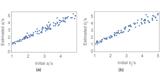
Figure 1: Panel (a) shows the original versus the estimated parameters $a_{i}$’s with $MSE=0.0628806$, while Panel (b) shows the original versus the estimated parameters $b_{j}$’s with $MSE=0.0768382$.

We also applied the algorithm to migration data between 34 countries. Here $w_{ij}$ is proportional to the number of people in thousands who moved from country $i$ to country $j$ (to find jobs) during the year 2011, and it is normalized so that be in the interval (0,1). The estimated parameters are in Table 1.

In this context, $a_{i}$’s are related to the emigration and and $b_{i}$’s to the counter-immigration potentials. When $a_{i}$ is large, country $i$ has a relatively large potential for emigration. On the contrary, when $b_{i}$ is large, country $i$ tends to have a relatively large resistance against immigration.

i	Country	$a_{i}$	$b_{i}$		i	Country	$a_{i}$	$b_{i}$
1	Australia	0.26931	1475.	75242	18	Japan	0.23211	9926.	91644
2	Austria	0.27403	632.	81653	19	Korea	0.22310	4199.	25005
3	Belgium	0.33380	46.	01197	20	Luxembourg	0.17543	107.	91399
4	Canada	0.27383	2363.	23435	21	Mexico	0.26706	4655.	95370
5	Chile	0.21236	28940.	59777	22	Netherlands	0.37754	39.	52320
6	Czech Rep.	0.31188	470.	28651	23	New Zealand	0.20542	2568.	00582
7	Denmark	0.26514	847.	34887	24	Norway	0.22646	519.	12451
8	Estonia	0.23235	25602.	33371	25	Poland	0.62846	1106.	55946
9	Finland	0.29357	1100.	00568	26	Portugal	0.31011	1606.	59979
10	France	0.52721	37.	92122	27	Slovak Rep.	0.27871	42451.	19093
11	Germany	0.62020	1.	64064	28	Slovenia	0.19720	6824.	54028
12	Greece	0.29708	6319.	19184	29	Spain	0.39732	182.	47160
13	Hungary	0.31443	32750.	88310	30	Sweden	0.39627	57.	34509
14	Iceland	0.18051	2950.	72653	31	Switzerland	0.33611	4524.	67821
15	Ireland	0.27555	364.	52781	32	Turkey	0.25900	146175.	82805
16	Israel	0.25854	1926.	04551	33	United Kingdom	0.49301	48.	61626
17	Italy	0.50522	135.	14076	34	United States	0.38019	2433.	78269

Table 1: Estimated parameters for migration data, 2011

It should be noted again that edge-weighted graphs of this type very frequently model real-world directed networks.

Appendix

A. Properties of the digamma function

Though, we do not use it explicitly, the following approximation of the digamma function $\psi(x)=\frac{\partial\ln\Gamma(x)}{\partial x}=\frac{\Gamma^{\prime}(x)}{\Gamma(x)}$ $(x>0$) is interesting for its own right.

Lemma 1

$\psi(x)=\ln(x-\frac{1}{2})+{\cal O}\left(\frac{1}{x^{2}}\right)$ for $x>1$.

The statement of the lemma easily follows by Taylor expansion.

Lemma 2

$\frac{1}{\psi^{\prime}(x+y)}>\frac{1}{\psi^{\prime}(x)}+\frac{1}{\psi^{\prime}(y)}$ for $x,y>0$.

Proof. First we prove that the function $u(x)=\frac{1}{\psi^{\prime}(x)}$, $x\in(0,\infty)$ is strictly convex. Indeed, one can easily see that

$$u^{\prime\prime}(x)=\frac{-\psi^{\prime\prime\prime}(x)[\psi^{\prime}(x)]^{2}+2[\psi^{\prime\prime}(x)]^{2}\psi^{\prime}(x)}{[\psi^{\prime}(x)]^{4}},$$

and this is positive due to $\psi^{\prime}(x)>0$ and the fact that

$$\frac{[\psi^{\prime\prime}(x)]^{2}}{\psi^{\prime\prime\prime}(x)\psi^{\prime}(x)}>\frac{1}{2}.$$

Latter one is a particular case of Corollary 2.3 in [2].

Now, in view of $\lim_{x\to 0}\psi^{\prime}(x)=\infty$, we can extend $u$ continuously to 0 by setting $u(0)=0.$ Then $u$ is still strictly convex, and therefore, for every $x,y>0$ we have $u(x)=u(\frac{y}{x+y}\cdot 0+\frac{x}{x+y}\cdot(x+y))<\frac{y}{x+y}u(0)+\frac{x}{x+y}u(x+y)$. Consequently,

$$u(x)<\frac{x}{x+y}u(x+y),$$ (8)

and likewise,

$$u(y)<\frac{y}{x+y}u(x+y).$$ (9)

Adding (8) and (9) together, we get the statement of the lemma. $\square$

Lemma 3

The function $\psi(2x)-\psi(x)$, $x\in(0,\infty)$ is decreasing and its range is $(\ln 2,\infty)$.

Proof. It is easily seen by the identity $\psi(2x)=\frac{1}{2}\psi(x)+\frac{1}{2}\psi\left(x+\frac{1}{2}\right)+\ln 2$ which can be found in [1]. $\square$

In the last lemma we collect some limiting properties of the digamma function and its derivative, see, e.g., [1, 2, 3] for details.

Lemma 4

The digamma function $\psi$ is a strictly concave, smooth function on $(0,\infty)$ that satisfies the following limit relations:

$$\lim_{x\to 0+}\psi(x)=-\infty,\quad\lim_{x\to\infty}\psi(x)=\infty,\quad\lim_{x\to\infty}\psi^{\prime}(x)=0,$$

$$\lim_{x\to\infty}(\psi(x)-\ln x)=0,\quad\quad\lim_{x\to 0+}(\psi(2x)-\psi(x))=\infty.$$

B. Considerations on the boundary of the mean parameter space

In Section 2, we saw that the mean parameter space ${\cal M}$ consists of $2n$-tuples $(A_{1},\dots A_{n},B_{1},\dots,B_{n})$ obtained from the parameters $(\mathbb{a},\mathbb{b})=(a_{1},\dots a_{n},b_{1},\dots,b_{n})$ of the underlying beta-distributions by Equations (4).

Denoting by $L(\mathbb{a},\mathbb{b})=(A_{1}(\mathbb{a},\mathbb{b}),\dots,A_{n}(\mathbb{a},\mathbb{b}),B_{1}(\mathbb{a},\mathbb{b}),\dots,B_{n}(\mathbb{a},\mathbb{b}))$ this dependence, i.e., the $\Theta\to{\cal M}$ (one-to-one) mapping, a boundary point $\bar{L}=({\bar{A}}_{1},\dots,{\bar{A}}_{n},{\bar{B}}_{1},\dots,{\bar{B}}_{n})$ of $\cal M$ can be obtained as ${\bar{L}}=\lim_{k\to\infty}L(\mathbb{a}^{k},\mathbb{b}^{k})$, where $\mathbb{a}^{k}=(a^{k}_{1},\dots,a^{k}_{n})$, $\mathbb{b}^{k}=(b^{k}_{1},\dots,b^{k}_{n})$, and

$$\lim_{k\to\infty}a^{k}_{i} ={\bar{a}}_{i}\in[0,\infty],\quad i=1,\dots n;$$

$$\lim_{k\to\infty}b^{k}_{j} ={\bar{b}}_{j}\in[0,\infty],\quad j=1,\dots n.$$

In view of Lemma 4, only the ${\bar{a}}_{i},{\bar{b}}_{j}=\infty$ cases have relevance. The sequence $(\mathbb{a}^{k},\mathbb{b}^{k})$ can be chosen such that

$$\lim_{k\to\infty}\frac{a^{k}_{i}}{b^{k}_{j}}=x_{ij}\quad\textrm{with}\quad 0<x_{ij}<\infty,\quad\textrm{for}\quad i\neq j.$$ (10)

Then, using 4),

$${\bar{A}}_{i} =-\lim_{k\to\infty}\sum_{j\neq i}\left[\psi({a}^{k}_{i}+{b}^{k}_{j})-\psi({a}^{k}_{i})\right]=\lim_{k\to\infty}\sum_{j\neq i}\left[\ln({a}^{k}_{i})-\ln({a}^{k}_{i}+{b}^{k}_{j})\right]=\sum_{j\neq i}\ln\frac{x_{ij}}{1+x_{ij}},\quad i=1,\dots,n;$$

$${\bar{B}}_{j} =-\lim_{k\to\infty}\sum_{i\neq j}\left[\psi({a}^{k}_{i}+{b}^{k}_{j})-\psi({b}^{k}_{j})\right]=\lim_{k\to\infty}\sum_{i\neq j}\left[\ln({b}^{k}_{j})-\ln({a}^{k}_{i}+{b}^{k}_{j})\right]=\sum_{i\neq j}\ln\frac{1}{1+x_{ij}},\quad j=1,\dots,n.$$

These equations show that the boundary point $\bar{L}$ of $\cal M$ contains – in its coordinates – the row- and column-sums of the matrices $\mathbb{U}(\mathbb{W})$ ad $\mathbb{V}(\mathbb{W})$ respectively (see Section 2), where the general off-diagonal entry of the $n\times n$ edge-weight matrix $\mathbb{W}$ is $\frac{x_{ij}}{1+x_{ij}}$.

Observe that $2n-1$ $x_{ij}$’s can be chosen free, and all the others are obtainable from them. To see this, consider the complete bipartite graph on vertex classes $(a_{1},\dots,a_{n})$ and $(b_{1},\dots,b_{n})$, where to the edge connecting $a_{i}$ and $b_{j}$ we assign $\frac{a_{i}}{b_{j}}$. Choose a minimal spanning tree of this graph (it contains $2n-1$ edges), and consider the sequence of $(\mathbb{a}^{k},\mathbb{b}^{k})$’s satisfying condition (10). Then, as $k\to\infty$, the $x_{ij}$’s of the edges not included in the spanning tree can be obtained from the $x_{ij}$’s of the $2n-1$ edges included in the spanning tree. Therefore the row- and column-sums of the edge-weight matrix $\mathbb{W}$ of entries $\frac{x_{ij}}{1+x_{ij}}$ $(i\neq j)$ are on a $(2n-1)$-dimensional manifold in $\mathbb{R}_{-}^{2n}$, so they are on the boundary of the convex hull $\cal T$ of the possible sufficient statistics $(\mathbb{R},\mathbb{C})$. However, this boundary has zero Lebesgue measure, and so, zero probability with respect to the underlying absolutely continuous distribution.

C. Proof of Theorem 2

It suffices to prove that some induced matrix norm of the matrix of the first derivatives $\mathbb{J}$ of $f$ at $\hat{\bm{\theta}}$ is strictly less than 1. We prove this for the $L_{1}$-norm. From (6) we obtain that

$$\frac{\partial g_{i}}{\partial a_{i}}({\hat{\mathbb{a}}},{\hat{b}})=\frac{\displaystyle\frac{1}{n-1}\sum_{j\neq i}\psi^{\prime}({\hat{a}}_{i}+{\hat{b}}_{j})}{\displaystyle\psi^{\prime}\left[\psi^{-1}\left(\frac{1}{n-1}\sum_{j\neq i}\psi({\hat{a}}_{i}+{\hat{b}}_{j})+\frac{R_{i}}{n-1}\right)\right]}.$$ (11)

From (3) we have $\frac{1}{n-1}\sum_{j\neq i}\psi({\hat{a}}_{i}+{\hat{b}}_{j})+\frac{R_{i}}{n-1}=\psi({\hat{a}}_{i})$. Substituting it into (11), we get

$$\frac{\partial g_{i}}{\partial a_{j}}({\hat{\mathbb{a}}},{\hat{b}})=\left\{\begin{array}[]{ll}\frac{\displaystyle\sum_{s\neq i}\frac{1}{n-1}\psi^{\prime}({\hat{a}}_{i}+{\hat{b}}_{s})}{\displaystyle\psi^{\prime}({\hat{a}}_{i})}&\mbox{\ if\ }j=i\\ 0&\mbox{\ if\ }j\neq i.\end{array}\right.$$

Likewise,

$$\frac{\partial g_{i}}{\partial b_{j}}({\hat{\mathbb{a}}},{\hat{b}})=\left\{\begin{array}[]{ll}0&\mbox{\ if\ }j=i\\ \frac{\displaystyle\frac{1}{n-1}\psi^{\prime}({\hat{a}}_{i}+{\hat{b}}_{j})}{\displaystyle\psi^{\prime}({\hat{a}}_{i})}&\mbox{\ if\ }j\neq i.\end{array}\right.$$

Further,

$$\frac{\partial h_{i}}{\partial a_{j}}({\hat{\mathbb{a}}},{\hat{b}})=\left\{\begin{array}[]{ll}0&\mbox{\ if\ }j=i\\ \frac{\displaystyle\frac{1}{n-1}\psi^{\prime}({\hat{a}}_{j}+{\hat{b}}_{i})}{\displaystyle\psi^{\prime}({\hat{b}}_{i})}&\mbox{\ if\ }j\neq i\end{array}\right.$$

and

$$\frac{\partial h_{i}}{\partial b_{j}}({\hat{\mathbb{a}}},{\hat{\mathbb{b}}})=\left\{\begin{array}[]{ll}\frac{\displaystyle\sum_{s\neq i}\frac{1}{n-1}\psi^{\prime}({\hat{a}}_{s}+{\hat{b}}_{i})}{\displaystyle\psi^{\prime}({\hat{b}}_{i})}&\mbox{\ if\ }j=i\\ 0&\mbox{\ if\ }j\neq i.\end{array}\right.$$

Observe that $J({\hat{\mathbb{a}}},{\hat{b}})$ has nonnegative entries. Therefore, its $L_{1}$-norm is the maximum of its column-sums. The $j$th column-sum of $J({\hat{\mathbb{a}}},{\hat{b}})$ is equal to

$$\frac{\displaystyle\sum_{s\neq j}\frac{1}{n-1}\psi^{\prime}({\hat{a}}_{j}+{\hat{b}}_{s})}{\displaystyle\psi^{\prime}({\hat{a}}_{j})}+\sum_{s\neq j}\frac{\displaystyle\frac{1}{n-1}\psi^{\prime}({\hat{a}}_{j}+{\hat{b}}_{s})}{\displaystyle\psi^{\prime}({\hat{b}}_{s})}=\frac{1}{n-1}\sum_{s\neq j}\displaystyle\psi^{\prime}({\hat{a}}_{j}+{\hat{b}}_{s})\left(\displaystyle\frac{1}{\psi^{\prime}({\hat{a}}_{j})}+\frac{1}{\displaystyle\psi^{\prime}({\hat{b}}_{s})}\right)$$ (12)

for $j=1,\dots,n$; and likewise, the $(n+j)$th column-sum of $J({\hat{\mathbb{a}}},{\hat{b}})$ is

$$\frac{1}{n-1}\sum_{s\neq j}\displaystyle\psi^{\prime}({\hat{a}}_{s}+{\hat{b}}_{j})\left(\displaystyle\frac{1}{\psi^{\prime}({\hat{a}}_{s})}+\frac{1}{\displaystyle\psi^{\prime}({\hat{b}}_{j})}\right)$$ (13)

for $j=1,\dots,n$. As (12) and (13) are of similar appearance, it suffices to prove that the right hand side of (12) is less than 1. But $\displaystyle\psi^{\prime}({\hat{a}}_{j}+{\hat{b}}_{s})\left(\displaystyle\frac{1}{\psi^{\prime}({\hat{a}}_{j})}+\frac{1}{\displaystyle\psi^{\prime}({\hat{b}}_{s})}\right)<1$ holds by Lemma 2, and we have $n-1$ terms in the summation.

Since $f:\mathbb{R}^{2n}\to\mathbb{R}^{2n}$ is continuously differentiable in a neighborhood of ${\hat{\bm{\theta}}}=({\hat{\mathbb{a}}},{\hat{\mathbb{b}}})$, Theorem 3 of [7] implies that there is a closed neighborhood $K$ of $\hat{\bm{\theta}}$ such that $f$ is a contraction on $K$. In particular, the fixed point iteration $f(\bm{\theta}^{(it-1)})=\bm{\theta}^{(it)}$ $(it\to\infty)$ converges for every $\bm{\theta}^{(0)}\in K$ to $\hat{\bm{\theta}}$, which is the unique solution of (6). $\square$

References

- [1] Abramowitz, M., Stegun, I. A., eds., Handbook of Mathematical Functions with Formulas, Graphs, and Mathematical Tables (10th ed.). New York: Dover (1972), pp. 258-259.
- [2] Alzer, H., Wells, J., Inequalities for the polygamma functions, SIAM J. Math. Anal. 29 (6) (1998), 1459-1466.
- [3] Bernardo, J. M., Psi (digamma) function. Algorithm AS 103, Applied Statistics 25 (1976), 315–317.
- [4] Bolla, M., Spectral clustering and biclustering. Wiley (2013).
- [5] Bolla, M., Elbanna, A., Estimating parameters of a probabilistic heterogeneous block model via the EM algorithm, Journal of Probability and Statistics (2015), Article ID 657965.
- [6] Chatterjee, S., Diaconis, P. and Sly, A., Random graphs with a given degree sequence, Ann. Stat. 21 (2010), 1400–1435.
- [7] Grasmair, M., Fixed point iterations, https://wiki.math.ntnu.no/_media/ma2501/2014v/fixedpoint.pdf
- [8] C. J. Hillar, A. Wibisono, Maximum entropy distributions on graphs, arXiv:1301.3321v2 (2013).
- [9] Lauritzen, S. L., Graphical Models. Oxfor Univ. Press (1995).
- [10] Yan, T., Leng, C., Zhu, J., Asymptotics in directed exponential random graph models with an increasing bi-degree sequence, Ann. Stat. (2016) 44, 31-57.
- [11] M. Wainwright,. M. I. Jordan, Graphical models, exponential families, and variational inference, Foundations and Trends in Machine Learning 1 (1-2), 1-305 (2008).