Methods for compressible fluid simulation on GPUs using high-order finite differences

Abstract

We focus on implementing and optimizing a sixth-order finite-difference solver for simulating compressible fluids on a GPU using third-order Runge-Kutta integration. Since graphics processing units perform well in data-parallel tasks, this makes them an attractive platform for fluid simulation. However, high-order stencil computation is memory-intensive with respect to both main memory and the caches of the GPU. We present two approaches for simulating compressible fluids using 55-point and 19-point stencils. We seek to reduce the requirements for memory bandwidth and cache size in our methods by using cache blocking and decomposing a latency-bound kernel into several bandwidth-bound kernels. Our fastest implementation is bandwidth-bound and integrates $343$ million grid points per second on a Tesla K40t GPU, achieving a $3.6\times$ speedup over a comparable hydrodynamics solver benchmarked on two Intel Xeon E5-2690v3 processors. Our alternative GPU implementation is latency-bound and achieves the rate of $168$ million updates per second.

©2017. This manuscript version is made available under the CC-BY-NC-ND 4.0 license, http://creativecommons.org/licenses/by-nc-nd/4.0/

Publisher DOI: 10.1016/j.cpc.2017.03.011

1 Introduction

The number of transistors in a microprocessor has been doubling approximately every two years and as a result, the performance of supercomputers measured in floating-point operations per second (FLOPS) has been following a similar increase. However, since increasing the clock frequencies of microprocessors to gain better performance is no longer feasible because of power constraints, this has lead to a change in their architectures from single-core to multi-core.

While modern central processing units (CPUs) utilize more cores and wider SIMD units, they are designed to perform well in general tasks where low memory access latency is important. On the other hand, graphics processing units (GPUs) are specialized in solving data-parallel problems found in real-time computer graphics and as a result, house more parallel thread processors and use higher-bandwidth memory than CPUs. With the introduction of general-purpose programming frameworks, such as OpenCL and CUDA, GPUs can now also be programmed to do general purpose tasks using a C-like language instead of using a graphics application-programming interface (API), such as OpenGL. In addition, APIs such as OpenACC can be used to convert existing CPU programs to work on a GPU. For these reasons, GPUs offer an attractive platform for physical simulations which can be solved in a data-parallel fashion.

In this work we concentrate on investigating sixth-order central finite-difference scheme implementations on GPUs, suitable for multiphysics applications. The justification for the use of central differences with explicit time stepping, a configuration which is not ideal concerning its stability properties, comes from the fact that, even though some amount of diffusion is required for stability, they provide very good accuracy and are easy to implement (see, e.g. [1]). In addition, the various types of boundary conditions and grid geometries needed in multiphysics codes such as the Pencil Code are easy to implement with central schemes. Moreover, the problem has the potential to exhibit strong scaling with the number of parallel cores in the optimal case.

There are astrophysical hydro- and magnetohydrodynamic solvers already modified to take advantage of accelerator platforms (i.e. [2], [3], [4]), that most often use low-order discretization. As an example of a higher-order scheme for cosmological hydrodynamics, we refer to [5]. We also note that more theoretical than application-driven work on investigating higher-order stencils on GPU architecture exists in the literature, see e.g. [6]. There are many scientific problems, such as modeling hydromagnetic dynamos, where long integration times are required, either to reach a saturated state (see e.g. [7]), or to exhibit non-stationary phenomena and secular trends (see e.g. [8]). Therefore, it is highly desirable to find efficient ways to accelerate the methods, GPUs offering an ideal framework. The accelerated codes typically employ lower-order conservative schemes, in which case the halo region to be communicated to compute the differences is small, and does not pose the main challenge for the GPU implementation. High-order schemes of similar type as presented here exist for two-dimensional hydrodynamics (e.g. [9]); in this paper, we deal with a 3D implementation of a higher-order finite-difference solver. Such schemes are much less diffusive and they are more suitable for accurate modeling of turbulence, which is, on the other hand, crucial for e.g. investigating various types of instabilities in astrophysical settings. One mundane example, which is the solar dynamo, is responsible for all the activity phenomena on the Sun, driving the space weather and climate that affect life on Earth [10]. The accurate modeling of turbulence is also important in understanding such phenomena as the structure of interstellar medium [11] and star formation [12].

We make the following contributions in this work. First, we describe, implement and optimize two novel methods for simulating compressible fluids on GPUs using sixth-order finite differences and 19- and 55-point stencils. The current implementation is for simulations of isothermal fluid turbulence. The bigger picture is that it uses the same core methods as the Pencil Code. Thus the current code development works as a pilot project in the conversion of the Pencil Code to use GPUs.

Our implementations perform $1.7\times$ and $3.6\times$ faster than a state-of-the-art finite difference solver, Pencil Code, used for scientific computation on HPC-clusters. Second, we present an optimization technique called kernel decomposition, which can be used to improve the performance of latency-bound kernels. Currently our code, called Astaroth, supports isothermal compressive hydrodynamics, but it will be expanded in the future to include more complex physics, in the end supporting the full equations of magnetohydrodynamics (MHD).

In this paper, we present the physical motivation (Sect. 2) behind our implementations, and the technical justification and background (Sect. 3). The details of our implementations and the Astaroth code are presented in Sect. 4. In Sect. 5 we present the performance of our GPU implementations and compare the results with physical test cases in Sect. 6. Finally, in Sect. 7, we discuss our results and conclude the paper.

2 Problem specification

Here we describe the basic equations and numerical methods featured in the current implementation of the Astaroth code, which were also used in testing the different optimizations. For simplicity, the code is limited to the domain of hydrodynamics. We consider the fluid to be isothermal and compressible, and we include the full formulation of viscosity to the momentum equation. This allows for testing our methods with reasonable enough physics while avoiding overt complexity during the development of the methods.

2.1 Governing equations

In a compressible system, the conservation of mass can be expressed as the rate equation for density $\rho$, called the continuity equation:

$$\frac{D\ln\rho}{Dt}=-\nabla\cdot\mathbf{u}.$$ (1)

Here $D/Dt$ is the convective derivative $\partial/\partial t+(\mathbf{u}\cdot\nabla)$ and density is expressed in logarithmic form $\ln\rho$ and $\mathbf{u}$ is a three-dimensional velocity vector. The logarithmic form of density helps to avoid numerical errors that can occur with large stratifications or erroneously negative values of density.

Momentum conservation in a viscous fluid is modelled by a rate equation commonly known as the Navier-Stokes equation. In the case of isothermal viscous hydrodynamics featured in the Astaroth code it is given by:

$$\frac{D\mathbf{u}}{Dt}=-c_{s}^{2}\nabla\ln\rho+\mathbf{f}+\nu\bigg{(}\nabla^{2}\mathbf{u}+\frac{1}{3}\nabla(\nabla\cdot\mathbf{u})+2\mathbf{S}\cdot\nabla\ln\rho\bigg{)},$$ (2)

where $-c_{s}^{2}\nabla\ln\rho$ is the pressure term in the isothermal case where the pressure is given by $p=\rho c_{s}^{2}$ with $c_{s}$ being the constant sound speed, $\mathbf{f}$ is an external body force, such as an external gravity field or a forcing function (see Sect. 6), $\nu$ is the kinematic viscosity coefficient, which is assumed constant, and $\mathbf{S}$ is the traceless rate-of-strain tensor:

$$S_{ij}=\frac{1}{2}\bigg{(}\frac{\partial u_{i}}{\partial x_{j}}+\frac{\partial u_{j}}{\partial x_{i}}-\frac{2}{3}\delta_{ij}\nabla\cdot\mathbf{u}\bigg{)}.$$ (3)

2.2 Non-dimensional units and system parameters

While solving the equations, we assume that the variables are described in dimensionless manner. Depending on the nature of the actual physical question, the result can be scaled during the data analysis phase into relevant physical dimensions. In this way, we can avoid using numerically unsound parameter values.

The dimensionless physical units are defined as

$$\begin{split}\rho=\frac{\rho_{\mathrm{phys}}}{M_{\mathrm{u}}/L_{\mathrm{u}}^{3}},&\quad\mathbf{u}=\frac{\mathbf{u}_{\mathrm{phys}}}{L_{\mathrm{u}}/T_{\mathrm{u}}},\quad\nu=\frac{\nu_{\mathrm{phys}}}{L_{\mathrm{u}}^{2}/T_{\mathrm{u}}},\\ c_{s}=\frac{c_{s\mathrm{,phys}}}{L_{\mathrm{u}}/T_{\mathrm{u}}},&\quad k=\frac{k_{\mathrm{phys}}}{2\pi/L_{\mathrm{u}}}\end{split}$$ (4)

where $L_{\mathrm{u}}$, $M_{\mathrm{u}}$ and $T_{\mathrm{u}}$ denote chosen unit scaling of length, mass and time respectively.

In addition, we use an important dimensionless measure, the Reynolds number,

$$\mathrm{Re}=\frac{uL}{\nu}$$ (5)

where $u$ and $L$ represent characteristic velocities and length scales in the system.

2.3 The finite difference method

We discretize the fluid volume $(L_{x},L_{y},L_{z})$ onto an equidistant grid of $(N_{x},N_{y},N_{z})$ points, the distance between neighbouring grid points in each dimension being $\delta_{i}=L_{i}/N_{i}$. With these, the approximation of the first derivative of function $f$ on the grid point $i$ with respect to the $x$-direction when using sixth-order central differences can be written as follows [1, pp. 5–7].

$$\begin{split}\frac{\partial}{\partial x}f_{i}=\frac{1}{60\delta_{x}}\biggl{(}&-f_{i-3}+9f_{i-2}-45f_{i-1}\\ &+45f_{i+1}-9f_{i+2}+f_{i+3}\biggr{)}+O(\delta_{x}^{6})\ .\end{split}$$ (6)

The second derivatives can be approximated with

$$\begin{split}\frac{\partial^{2}}{\partial x^{2}}f_{i}=\frac{1}{180\delta_{x}}\biggl{(}&2f_{i-3}-27f_{i-2}+270f_{i-1}-490f_{i}\\ &+270f_{i+1}-27f_{i+2}+2f_{i+3}\biggr{)}+O(\delta_{x}^{6})\ .\end{split}$$ (7)

Additionally, mixed derivatives with respect to any two arbitrary directions can be approximated by using the following bidiagonal scheme [13], here with respect to $x$- and $y$-directions.

$$\begin{split}\frac{\partial^{2}}{\partial x\partial y}f_{i,j}=\frac{1}{720\delta_{x}\delta_{y}}&\biggl{[}270(f_{i+1,j+1}-f_{i-1,j+1}+f_{i-1,j-1}-f_{i+1,j-1})\\ &-27(f_{i+2,j+2}-f_{i-2,j+2}+f_{i-2,j-2}-f_{i+2,j-2})\\ &+2(f_{i+3,j+3}-f_{i-3,j+3}+f_{i-3,j-3}-f_{i+3,j-3})\biggr{]}\\ &+O(\delta_{x}^{6},\delta_{y}^{6})\ .\end{split}$$ (8)

Finally, we can approximate second and mixed derivatives using Eq. (6) as follows

$$\frac{\partial}{\partial x}(\frac{\partial}{\partial y}f_{i,j})=\frac{1}{60\delta_{x}}\biggl{[} -\biggl{(}\frac{\partial}{\partial y}f_{i-3,j}\biggr{)}+9\biggl{(}\frac{\partial}{\partial y}f_{i-2,j}\biggr{)}-45\biggl{(}\frac{\partial}{\partial y}f_{i-1,j}\biggr{)}$$ (9)

$$+45\biggl{(}\frac{\partial}{\partial y}f_{i+1,j}\biggr{)}-9\biggl{(}\frac{\partial}{\partial y}f_{i+2,j}\biggr{)}+\biggl{(}\frac{\partial}{\partial y}f_{i+3,j}\biggr{)}\biggr{]}$$

$$+O(\delta_{x}^{6})\ .$$

Computing the derivatives of a grid point requires information from its neighboring grid points. This data access pattern is called a $k$-point stencil, where data from $k$ input points is read in order to update the output point. We use $R$ to denote the radius of the stencil, which is the Chebychev distance from the output point to the farthest input point of the stencil. For central differences, the relation between the radius of the stencil $R$ and the order of the finite difference method $n$ is thus $n=2R$. Additionally, a function solving only the first- and second-order derivatives in $d\geq 1$ dimensions using an $n$th-order central finite difference method uses a $(dn+1)$-point stencil to update a grid point, whereas a function, which computes also the mixed derivatives requires a $(dn+2\binom{d}{2}n+1)$-point stencil for $d\geq 2$. The stencils used in such functions are shown in Fig. 1.

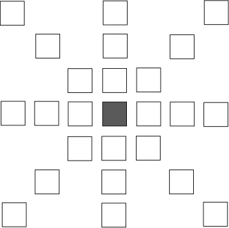
Figure 1: Two-dimensional cuts of the stencils used in the functions, which approximate derivatives using sixth-order finite differences. A 19-point stencil (left) is used in a function, which solves only first- and second-order derivatives, whereas a 55-point stencil (right) is used in a function, which computes also mixed derivatives using the bidiagonal scheme. The white and dark cells are input and output points, respectively. For both stencils, $R=3$.

2.4 Runge-Kutta integration

Our implementations are based on an explicit third-order Runge-Kutta formula, which is written as a $2N$-storage scheme [1, p. 9]. In this approach, only one set of intermediate values have to be memory-resident during integration.

Let $\mathbf{u}$ be a vector field the integration is performed on and $\widetilde{\mathbf{u}}$ be the field containing the intermediate values. Additionally, let $\mathbf{u}^{(s)}$ be the value of $\mathbf{u}$ during integration substep $s$. Finally, $\alpha^{(s)}$ and $\beta^{(s)}$ are coefficients whose values depend on the chosen 2N-RK3 scheme and $\delta_{t}$ is the length of the time step.

We can now write the 2N-RK scheme as

$$\widetilde{\mathbf{u}}^{(s+1)}=\alpha^{(s)}\widetilde{\mathbf{u}}^{(s)}+\frac{\partial}{\partial t}\mathbf{u}^{(s)}\delta_{t}\qquad\mathbf{u}^{(s+1)}=\mathbf{u}^{(s)}+\beta^{(s)}\widetilde{\mathbf{u}}^{(s+1)}\ .$$ (10)

The pseudocode for a naïve integration with this scheme is shown in Algorithm 1. Here $\widetilde{\rho}_{i}$ and $\widetilde{\mathbf{u}}_{i}$ are the intermediate results for density and velocity of a grid point at index $i$. Handling of the out-of-bound indices depends on the chosen boundary condition scheme. For the first step, $\alpha^{(1)}$ must be set to $0$.

Algorithm 1 Third-order 2N-storage Runge-Kutta integration

0:  Integer $i$ belongs to the set of indices in the computational domain $D$.

  for integration substep s = 1 to 3  do

     Compute boundary conditions for $\rho$ and $\mathbf{u}$

     for all $i\in D$ in parallel do

        $\widetilde{\rho}_{i}\leftarrow\alpha^{(s)}\widetilde{\rho}_{i}+\delta t\frac{\partial}{\partial t}\rho_{i}$

        $\widetilde{\mathbf{u}}_{i}\leftarrow\alpha^{(s)}\widetilde{\mathbf{u}}_{i}+\delta t\frac{\partial}{\partial t}\mathbf{u}_{i}$

     end for

     for all $i\in D$ in parallel do

        $\rho_{i}\leftarrow\rho_{i}+\beta^{(s)}\widetilde{\rho}_{i}$

        $\mathbf{u}_{i}\leftarrow\mathbf{u}_{i}+\beta^{(s)}\widetilde{\mathbf{u}}_{i}$

     end for

  end for

3 GPU architecture

In this section, we review GPU architecture using NVIDIA’s CUDA as the framework of choice and discuss the challenges of high-order stencil computation on GPUs. While we use terminology associated with CUDA, the ideas represented here are also analogous with those found in OpenCL and computer architecture in general. We denote the alternative terminology in the footnotes. Throughout this work, we use NVIDIA’s compute capability 3.5 GPUs as the baseline architecture.

Graphics processing units operate in a multi-threaded SIMD fashion and are designed to perform well in data-parallel tasks. In order to maximize throughput in these types of tasks, GPUs employ a large number of parallel thread processors and use specialized GDDR SGRAM to increase memory bandwidth with the cost of increased access latency. Modern GPUs also employ small L1 and L2 caches to reduce pressure to the on-device memory. See Table 1 for the detailed specifications of a Tesla K40t accelerator card used in this work. In order to hide pipeline and memory access latencies, GPUs rely mainly on multithreading a large number of threads on their processors in a fine-grained fashion. Alternatively, in certain problems instruction-level parallelism (ILP) can be used for the same latency-hiding effect [14].

Modern NVIDIA GPUs consist of Streaming Multiprocessors (SMX), which execute warps of CUDA threads. In current NVIDIA architectures, a warp is composed of $32$ threads. The threads of a warp are executed in lockstep on the thread processors of an SMX. Finally, sets of warps form thread blocks, which are distributed among SMXs by a thread block scheduler. For a more detailed description of the architecture of GPUs, we refer the reader to [15] and [16].

Table 1: Tesla K40t specifications rounded to two decimal places.

	Tesla K40t
GPU chip	GK110BGL
Compute capability	3.5
GPU memory (GDDR5 SGRAM)	12288 MiB
Memory bus width	384 bits
Peak memory clock rate	3004 MHz
Theoretical memory bandwidth	268.58 GiB/s
Number of SMX processors	15
Max 32-bit registers per SIMD processor	65 536
Max shared memory per thread block	49 152 bytes
L2 cache size	1.50 MiB

3.1 Related work and optimization techniques

Optimization of GPU programs is often non-trivial and requires careful tuning to attain the highest throughput. Techniques for optimizing low-order stencil computation have been studied extensively in literature, e.g. by [17] [18] [19] [20] [21], while work on higher-order stencil computation is more limited [22] [23] and focuses on stencils, where only the axis-aligned elements are used during an update. To our knowledge, no previous work has been published on optimizing 55-point stencil computation using stencil elements of size $16$ bytes and larger.

Memory bandwidth is a common bottleneck in stencil computation because of the low bandwidth-to-compute ratio in current microprocessor architectures. Previous work has suggested several techniques for reducing bandwidth requirements, notably spatial cache blocking techniques which aim to reduce memory fetches by reusing as much of the data as possible before evicting it out of caches. We also adopted this idea in our implementations we discuss in detail in Sect. 4.1 and 4.2.

However, with higher-order stencils more data is required to be cache-resident in order to improve performance with cache blocking. Using large amounts of shared memory in a kernel reduces its occupancy, which in turn results in decreased ability to hide latencies if increasing ILP in the kernel is not possible. In current GPU architectures, the cache size is insufficient for housing large three-dimensional blocks of $16$-byte-sized grid points.

4 GPU Implementations

Here we give an overview of our GPU implementations and the optimizations performed upon both implementations. First, we discretize the simulation domain into a grid as described in Sect. 2.3. The grid consists of a computational domain, which is surrounded by a ghost zone. We update the grid points in the computational domain using third-order Runge-Kutta integration, while the ghost zone is used to simplify integration near the boundaries. After each integration step, a number of grid points are copied from the computational domain into the ghost zone according to the boundary conditions. With this approach, we do not have to compute the boundary conditions within the integration kernel and can thus update all grid points in the computational domain using the same code. We use periodic boundary conditions throughout this work.

We store density $\rho$, velocity $\mathbf{u}$ and the intermediate result arrays $\widetilde{\rho}$ and $\widetilde{\mathbf{u}}$ into global memory as a structure of arrays. Arrays $\rho$ and $\mathbf{u}$ include the ghost zone and are padded manually, such that the first grid point of the computational domain is stored in a memory address which is a multiple of 128 bytes. By padding, we seek to reduce the number of memory transactions required to update the grid, which is discussed more in detail in Sect. 5. In order to avoid a race condition during integration, we allocate memory for arrays $\rho$, $\mathbf{u}$, $\rho^{\text{out}}$ and $\mathbf{u}^{\text{out}}$, such that separate arrays are used for reading and writing. Arrays $\rho$ and $\mathbf{u}$ are passed to the integration kernels using the const __restrict__ intrinsic, which enables these arrays to be read through the read-only texture cache. Additionally, we store all constants discussed in Sect. 2 into constant memory. Finally, in both our integration kernels, we compute each derivative only once and store each value, which is used more than once, into either shared memory or registers.

4.1 55-point integration method

We solve the problem on a GPU using a modified version of Algorithm 1. The difference is, that we use separate arrays for reading and writing and thus can update the computational domain in one pass over the grid points. At the end of each integration substep, the arrays are swapped efficiently using pointers.

In our modified integration algorithm, we update a grid point by solving the continuity and Navier-Stokes equations, Eq. (1) and (2), within a single kernel. As we solve the derivatives in these equations with the finite-difference equations (6), (7) and (8), the integration kernel requires a 55-point stencil in order to update a grid point. Therefore we call this approach the 55-point method. The pseudocode for the 55-point method is shown in Algorithm 2 using the notation introduced in Sections 2.4 and 4.

Algorithm 2 Integration with the 55-point method

0:  Integer $i$ belongs to the set of indices in the computational domain $D$.

  for integration step s = 1 to 3  do

     Compute boundary conditions for $\rho$ and $\mathbf{u}$

     for all $i\in D$ in parallel do

        $\widetilde{\rho}_{i}\leftarrow\alpha^{(s)}\widetilde{\rho}_{i}+\delta t\frac{\partial}{\partial t}\rho_{i}$

        $\widetilde{\mathbf{u}}_{i}\leftarrow\alpha^{(s)}\widetilde{\mathbf{u}}_{i}+\delta t\frac{\partial}{\partial t}\mathbf{u}_{i}$

        $\rho_{i}^{\text{out}}\leftarrow\rho_{i}+\beta^{(s)}\widetilde{\rho}_{i}$

        $\mathbf{u}_{i}^{\text{out}}\leftarrow\mathbf{u}_{i}+\beta^{(s)}\widetilde{\mathbf{u}}_{i}$

     end for

     $\rho\leftarrow\rho^{\text{out}}$

     $\mathbf{u}\leftarrow\mathbf{u}^{\text{out}}$

  end for

The algorithm is implemented in CUDA as follows. Let $\tau_{x}$, $\tau_{y}$ and $\tau_{z}$ be the dimensions of a thread block and $R$ the radius of the stencil as defined in Sect. 2.3. We perform the integration by decomposing the computational domain into $\tau_{x}\times\tau_{y}\times\tau_{z}$-sized blocks, where each grid point is updated by a CUDA thread. Since the stencils used to update nearby grid points overlap, we can reduce global memory fetches by fetching the data used by the threads in a thread block into shared memory.

The block of grid points stored into shared memory per a thread block is shown in Fig. 2. We call the area surrounding the shared memory block a halo in order to distinguish it from the ghost zones discussed in Sect. 4. Unlike ghost zones, the boundary conditions are not applied to the halo and the grid points in the halo are solely used for updating the grid points near the boundaries of the thread block. For simplicity, we fetch a total of $(\tau_{x}+2R)\times(\tau_{y}+2R)\times(\tau_{z}+2R)$ grid points into shared memory per a thread block, even when some of the grid points are used only by a single thread or none at all. This approach avoids branching in the integration kernel, as all threads follow the same execution path with the cost of additional memory fetches. We discuss these redundant memory fetches more in detail in Sect. 7.

In order to reduce the number of memory transactions from global memory, we adopted the idea of a rolling cache. In this approach, part of the data in shared memory is reused for updating multiple grid points along the $z$-axis. We implemented cache blocking for Alg. 2 as follows.

Initial step:
(a) Assign a block of grid points in the decomposed computational domain to a CUDA thread block.
(b) Fetch the data required for updating this block of grid points from global memory into shared memory.
(c) Update the block of grid points using the data stored in shared memory.

Subsequent steps: While a thread block has updated less than $E_{z}$ blocks of grid points, do the following:
(d) Assign the next block of grid points in the $z$-axis to the thread block.
(e) Since the halos of nearby blocks overlap, part of the data obtained in the previous step can also be used to update the current block of grid points. Hold this data in shared memory. Load rest of the required data from global memory into shared memory.
(f) Update the assigned block of grid points using the data in shared memory.

In our implementation of the rolling cache, we avoid copying data around shared memory by using a counter indicating the current mid-point in the shared memory block. After updating a grid point, we increment this counter by $\tau_{z}$ in modulo $\tau_{z}+2R$. During differentiation, any out-of-bound indices encountered when accessing shared memory are also wrapped around modulo $\tau_{z}+2R$.

Additionally, let $N_{x}$, $N_{y}$ and $N_{z}$ be the dimensions of the computational domain and $E_{z}$ the number of grid points updated by a CUDA thread. The total number of thread blocks required to update the grid is thus

$$\gamma=\frac{N_{x}}{\tau_{x}}\cdot\frac{N_{y}}{\tau_{y}}\cdot\frac{N_{z}}{\tau_{z}E_{z}}\ ,$$ (11)

and the number of grid points fetched from global memory is

$$\Gamma_{55p}=(\tau_{x}+2R)\times(\tau_{y}+2R)\times(\tau_{z}E_{z}+2R)\ .$$ (12)

With the 55-point method, we perform the following number of read-writes $RW_{55p}$ to global memory when $N_{xyz}=N_{x}N_{y}N_{z}$. Here we read from four arrays which require the halo ($\rho$ and $\mathbf{u}$) and four intermediate value arrays ($\widetilde{\rho}$ and $\widetilde{\mathbf{u}}$), and write the result back to eight arrays ($\rho^{\text{out}}$, $\mathbf{u}^{\text{out}}$, $\widetilde{\rho}$ and $\widetilde{\mathbf{u}}$).

$$RW_{55p}=\underbrace{4\Gamma_{55p}\gamma+4N_{xyz}}_{\text{Reads}}+\underbrace{8N_{xyz}}_{\text{Writes}}\ .$$ (13)

However, the main problem with the 55-point method is low occupancy caused by the large amount of shared memory required by a thread block in order to benefit from cache blocking. This is the case also for small thread blocks. For example, when using thread blocks of size $\tau_{x}=\tau_{y}=\tau_{z}=8$, $R=3$ and storing $16$ bytes of information per grid point, then a thread block requires $43\ 904$ bytes of the $49\ 152$ bytes available shared memory on a Tesla K40t GPU. Therefore only one thread block can run on the GPU at a time. This is not enough to hide the latencies in our integration kernel, which becomes latency-bound. Moreover, instruction-level parallelism cannot be used extensively to hide the latencies in our approach, since the data in shared memory can be updated only after the threads of a thread block have updated their currently assigned grid points.

4.2 19-point integration method

To alleviate the problem with high shared memory usage in our 55-point method, we represent an alternative integration method which uses an axis-aligned 19-point stencil to update a grid point. This is achieved by computing the gradient of divergence in Eq. 2 in two passes over the grid. The benefit of this approach is, that stencil computation on GPU with axis-aligned stencils is extensively studied and efficient cache blocking methods for such stencils are well known [17] [18] [19]. However, the disadvantages of this approach compared with our 55-point method are three-fold: first, we have to perform more floating-point arithmetic in order to update a grid point, which introduces a slight error. We show in Sect. 6 that this error is negligible. Second, as the grid is updated in two steps, more memory transactions are required to complete a single integration step. Third, when solving the system with multiple GPUs, part of the divergence field has to be communicated between the nodes.

The 19-point method works as follows. First, we reformulate the Navier-Stokes equation in such form, that mixed derivatives do not have to be solved in order to compute the gradient of divergence. This is achieved by dividing a substep of a full integration step into two passes, where the divergence field is solved during the first pass and during the second pass, the gradient of divergence is solved using the precomputed divergence field. The complete reformulation of the Navier-Stokes equation is shown in Appendix A. Using the notation from Sect. 2.4 and $\widetilde{\mathbf{u}}_{partial}^{(s)}$ and $\mathbf{u}_{partial}^{(s)}$ to denote the partially computed Navier-Stokes equation, we can write the calculations done during the first pass as follows. Here $s$ denotes some substep of a full integration step. For RK3, $s\in\{1,2,3\}$.

$$\nabla\cdot\mathbf{u}^{(s)} =\frac{\partial}{\partial x}u+\frac{\partial}{\partial y}v+\frac{\partial}{\partial z}w$$ (14)

$$\widetilde{\mathbf{u}}_{partial}^{(s+1)} =\alpha^{(s)}\widetilde{\mathbf{u}}^{(s)}+\delta_{t}\biggl{[}-({\mathbf{u}}^{(s)}\cdot\nabla){\mathbf{u}}^{(s)}-c_{s}^{2}\nabla\ln\rho^{(s)}$$

$$+\nu\bigg{(}\nabla^{2}\mathbf{u}^{(s)}+2\mathbf{S}\cdot\nabla\ln\rho^{(s)}\biggr{)}\biggr{]}$$ (15)

$$\mathbf{u}_{partial}^{(s+1)} =\mathbf{u}^{(s)}+\beta^{(s)}\widetilde{\mathbf{u}}_{partial}^{(s+1)}\ ,$$ (16)

where $\mathbf{u}=(u,v,w)$.

Then, with the second pass we complete the integration step by computing $\widetilde{\mathbf{u}}^{(s+1)}$ and $\mathbf{u}^{(s+1)}$ using the previously computed divergence field and the partial results.

$$\widetilde{\mathbf{u}}^{(s+1)} =\widetilde{\mathbf{u}}_{partial}^{(s+1)}+\delta_{t}\frac{\nu}{3}\nabla(\nabla\cdot\mathbf{u}^{(s)})$$ (17)

$$\mathbf{u}^{(s+1)} =\mathbf{u}_{partial}^{(s+1)}+\beta^{(s)}\delta_{t}\frac{\nu}{3}\nabla(\nabla\cdot\mathbf{u}^{(s)})\ .$$ (18)

The pseudocode for this approach is shown in Algorithm 3.

Algorithm 3 Integration with the 19-point method

0:  Integer $i$ belongs to the set of indices in the computational domain $D$.

  for integration step s = 1 to 3  do

     Compute boundary conditions for $\rho$ and $\mathbf{u}$

     for all $i\in D$ in parallel do

        $(\nabla\cdot\mathbf{u})_{i}\leftarrow\frac{\partial}{\partial x}u_{i}+\frac{\partial}{\partial y}v_{i}+\frac{\partial}{\partial z}w_{i}$

        $\widetilde{\rho}_{i}\leftarrow\alpha^{(s)}\widetilde{\rho}_{i}+\delta t\frac{\partial}{\partial t}\rho_{i}$

        $\widetilde{\mathbf{u}}_{i}\leftarrow\alpha^{(s)}\widetilde{\mathbf{u}}_{i}+\delta_{t}\biggl{[}-(\mathbf{u}_{i}\cdot\nabla)\mathbf{u}_{i}-c_{s}^{2}\nabla\ln\rho_{i}+\nu\bigg{(}\nabla^{2}\mathbf{u}_{i}+2\mathbf{S}\cdot\nabla\ln\rho_{i}\biggr{)}\biggr{]}$

        $\rho_{i}^{\text{out}}\leftarrow\rho_{i}+\beta^{(s)}\widetilde{\rho}_{i}$

        $\mathbf{u}_{i}^{\text{out}}\leftarrow\mathbf{u}_{i}+\beta^{(s)}\widetilde{\mathbf{u}}_{i}$

     end for

     Compute boundary conditions for $(\nabla\cdot\mathbf{u})$

     for all $i\in D$ in parallel do

        $\widetilde{\mathbf{u}}_{i}\leftarrow\widetilde{\mathbf{u}}_{i}+\delta_{t}\frac{\nu}{3}\nabla(\nabla\cdot\mathbf{u})_{i}$

        $\mathbf{u}_{i}^{\text{out}}\leftarrow\mathbf{u}_{i}^{\text{out}}+\beta^{(s)}\delta_{t}\frac{\nu}{3}\nabla(\nabla\cdot\mathbf{u})_{i}$

     end for

     $\rho\leftarrow\rho^{\text{out}}$

     $\mathbf{u}\leftarrow\mathbf{u}^{\text{out}}$

  end for

We implemented the 19-point method in CUDA using the idea of 2.5D cache blocking [17] [18] to reduce the number of global memory transactions. In this approach, we set $\tau_{z}=1$ and store a 2-dimensional slab of data into shared memory, shown in Fig. 3. For simplicity, we allocate shared memory for $(\tau_{x}+2R)\times(\tau_{y}+2R)$ grid points, where the four $R^{2}$-sized corners of the slab are unused. Since the shared memory slab contains only grid points in the $xy$-plane, the rest of the stencil points required to solve the derivatives with respect to the $z$-axis are defined as local variables, which are placed into registers by the compiler. Similarly as in our 55-point method, each thread of a thread block then updates multiple grid points along the $z$-axis. Cache blocking works in our implementation as follows.

Initial step:
(a) Assign a 2-dimensional block of grid points to a thread block.
(b) Fetch the data required for solving the the derivatives in the $xy$-plane into shared memory and the data required for solving the derivatives in the $z$-axis into the registers of each thread.
(c) Update the block of grid points using the data in shared memory and registers.

Subsequent steps: While a thread block has updated less than $E_{z}$ blocks of grid points, do the following:
(d) Assign the next block of grid points in the $z$-axis to the thread block.
(e) Update the non-halo area of the shared memory slab using data stored in the registers of the threads and update the halo from global memory. For each thread, hold part of the data obtained in the previous steps in registers, but update the local variable corresponding to the stencil point furthest along the $z$-axis from global memory.
(f) Update the assigned block of grid points using the data in shared memory and registers.

Figure 2: A dissected shared memory block used by the 55-point method. The halo areas in the front and back of the block have been moved to left and right for clarity.

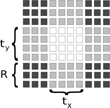
Figure 3: The shared memory slab used in the 19-point method. The stencil computation is performed on the grid points in the center. Grey cells represent the grid points in the halo while the black areas are unused.

Using the same notation as in Sect. 4.1 and $\tau_{z}=1$, the total number of grid points fetched from global memory by a thread block is

$$\Gamma_{19p}=\underbrace{\tau_{x}\tau_{y}E_{z}}_{\text{Computational area}}+\underbrace{2R(\tau_{x}\tau_{y}+\tau_{x}E_{z}+\tau_{y}E_{z})}_{\text{Halo area}}\ .$$ (19)

Additionally, by using Eq. 11 to solve the number of thread blocks $\gamma$ required to update the grid, we can now write the number of read-writes performed in the first and second pass as follows. During the first pass, we read-write to the same arrays as with the 55-point method in Eq. (13) with the addition of writing the divergence field to global memory. In the second pass, we read from one array including the halo ($\nabla\cdot\mathbf{u}^{(s)}$) and six partial result arrays ($\mathbf{\widetilde{u}}_{\text{partial}}$ and $\mathbf{u}_{\text{partial}}$), and write to six arrays ($\mathbf{\widetilde{u}}$ and $\mathbf{u}$).

$$RW_{19p,\text{1st pass}}=\underbrace{4\Gamma_{19p}\gamma+4N_{xyz}}_{\text{Reads}}+\underbrace{9N_{xyz}}_{\text{Writes}}$$ (20)

and

$$RW_{19p,\text{2nd pass}}=\underbrace{\Gamma_{19p}\gamma+6N_{xyz}}_{\text{Reads}}+\underbrace{6N_{xyz}}_{\text{Writes}}\ .$$ (21)

5 GPU performance

In this section, we present the results of our GPU implementations described in Sections 4.1 and 4.2. Additionally, we compare the performance of our implementations with the Pencil Code [13], which is a high-order finite-difference solver for compressible magnetohydrodynamic flows and is developed to run efficiently on multi-CPU hardware. We strived to benchmark both our GPU implementations in a comparable way by using equally optimized versions of both approaches. Additionally we compared the performance of our GPU implementations with the Pencil Code using equally modern hardware sold at similar price points. The performance of our GPU implementations is not compared with any other GPU finite-difference solver, because to our knowledge, no previous work has been done on simulating compressible fluids on GPUs using sixth-order finite-differences.

We generated the benchmarks for the implementations by running a test case, which simulated compressible hydrodynamic flow by using sixth-order finite differences and third-order Runge-Kutta integration. The benchmarks were run using single-precision floating-point numbers unless otherwise mentioned. Forcing was disabled in all performance tests. In order to get a fair comparison, we used grid sizes that are multiples of $12$ for generating the CPU results, since the workload in this case is divided more evenly on the $12$ cores of an Intel Xeon E5-2690v3 processor. In contrast, the optimal grid sizes shared by both of our GPU implementations are multiples of $32$, which we used to generate the GPU results. Diverging from our GPU implementations, Pencil Code uses a 2N-storage Runge-Kutta integration method which we described in Sect. 2.4. Therefore our 55-point method gives the same error as the Pencil Code, but our 19-point method does not. Additionally, we do not know whether the single-pass approach we used in our 55-point method would also be suitable for CPUs, and how it would affect the performance if used within the Pencil Code.

We tested our GPU implementations on an NVIDIA Tesla K40t accelerator card, based on a single 875-MHz Kepler GK110BGL GPU (15 SMXs, 192 CUDA cores per SMX, 745 MHz base clock rate). The on-device memory has a bus width of 384 bits and consists of a total of $12288$ MiB of GDDR5-3004 SDRAM (24 $\times$ 256MiB chips in clamshell mode), of which 11520 MiB is usable as global memory. Tests were performed with ECC enabled. A compute node consists of two 2.6-GHz Intel Xeon E5-2620-v2 Ivy Bridge CPUs (2.1 GHz base clock rate, 6 cores per CPU) with 32 GiB of DDR3-1600 memory and two NVIDIA Tesla K40t accelerator cards, which are connected via a 16x PCI Express 3.0 bus. We compiled the program with CUDA 6.5 and Intel 14.0.1 compiler (the only Intel compiler supported in CUDA 6.5) for compute capability 3.5 invoking nvcc with flags -ccbin icc, -O3 and -gencode arch=compute_35,code=sm_35.

The test case for Pencil Code was run on a compute node consisting of two 12-core 2.6-GHz Intel Xeon E5-2690v3 processors based on Haswell microarchitecture. Each core has 32 KiB of L1 cache and 768 KiB of L2 cache while a 30-MiB L3 cache is shared by the cores of the CPU. The main memory of a node consists of 8 $\times$ 16 GiB DDR4-2133 DIMMs. We used a revision of Pencil Code fetched on 2015-08-27 . This build was compiled with a Fortran 90 compiler for MPI programs invoked by the mpif90 command using -O3, -xCORE-AVX2, -fma, -funroll-all-loops and -implicitnone flags. We used Intel compiler version 15.0.2 and Intel MPI library version 5.0.2.

The performance comparison of our GPU implementations and the Pencil Code is shown in Fig. 4(a). We achieved the rate of $343$ million updates per second using the 19-point method, which was $2.0$ times faster than integration with the 55-point method, which achieved the update rate of $168$ million updates per second. The Pencil Code achieved an update rate of $51$ million updates per second using one CPU, while the update rate using two CPUs was $96$ million updates per second. With $256^{3}$-sized grids and single-precision, we achieved the best performance for the 19-point method by updating $16$ and $64$ grid points per thread in the first and second half of the algorithm, respectively. With double-precision and the 55-point method, we had to decrease the size of a thread block to $4\times 4\times 4$ threads in order to fit the required data into shared memory. In this case, the best performance was achieved when a total of $32$ grid points were updated by each thread. With double-precision, we achieved the rate of $25$ and $154$ million elements integrated per second with our 55-point and 19-point implementations, respectively.

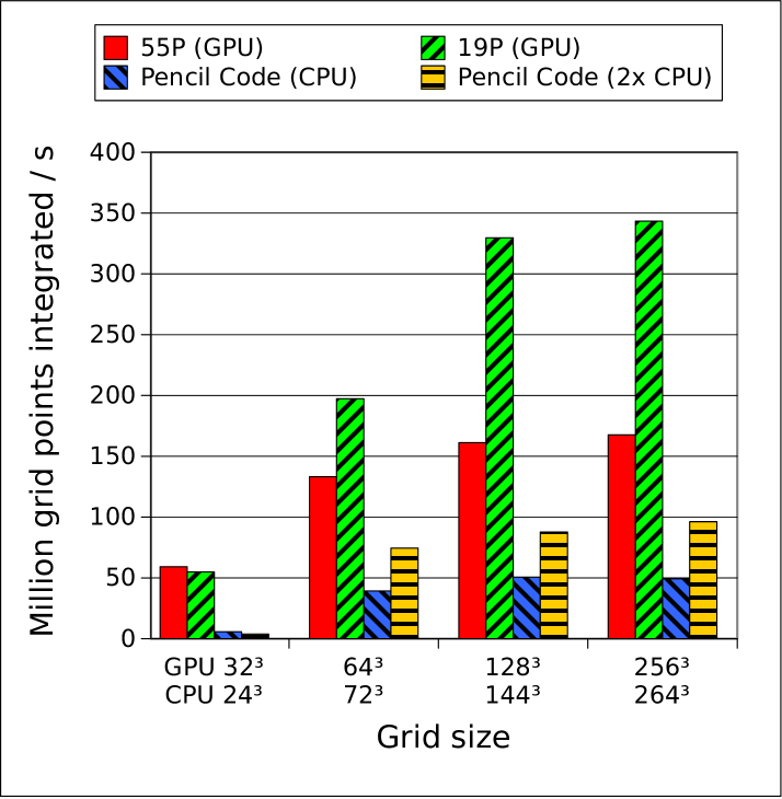
(a) Performance comparison.

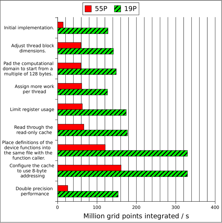
(b) Optimization steps and double-precision results.

Figure 4: (a) Performance comparison of the 19-point, 55-point methods and the CPU reference solver and (b) the optimizations performed upon the single-precision implementations and the double-precision results for our fastest solution, using a $128^{3}$-sized grid.

Fig. 4(b) shows the optimizations performed upon our GPU implementations. Notably, the performance decreases during the optimization step, where more work is added per thread. This is caused by overusing registers in the loop, which handles updating multiple grid points per thread, which in turn limits the occupancy of the integration kernel. As the next optimization step, we limited register usage with the __launch_bounds__ intrinsic, which causes any additional local variable above the limit to spill into L1 cache, but which in turn results in better performance because of the increased occupancy. Without adding more work per thread, we could not increase the performance by limiting register usage nor using the texture cache for reading. As the final optimization step, we moved the device functions used to compute derivatives from separately compiled modules to the same source file with the integration kernel, which resulted in a large boost in performance. The reason for this is, that when compiling a source, the compiler cannot optimize any calls to functions in separately compiled units, and must replace them with expensive calls which adhere to the application binary interface used in CUDA. With this step, we measured a $1.8\times$ and $1.9\times$ increase in performance of our 55-point and 19-point methods, respectively. We further improved the implementation of our 55-point method by setting the shared memory configuration to use eight-byte addressing mode, which resulted in a speedup of $34\%$. This step reduced the bandwidth requirement for L1 and shared memory, which was previously the limiting factor in the kernel. With the 19-point method, we did not see any notable difference in performance. The integration rate using double-precision is $2.1\times$ slower for the 19-point method and $6.3\times$ slower for the 55-point method. Because of the increased shared memory requirements, the latency issues in the 55-point method are accentuaded. In order to fit all the required data into shared memory, smaller thread blocks have to be used, which reduces both occupancy and the amount of data which can be reused. This causes the performance to degrade more than $2\times$ from the single-precision results. The 19-point method is still bound by memory bandwidth, even though the increased shared memory requirements limit the occupancy of the first half to $25\%$ or less regardless of the thread block dimensions.

Tables 2 and 3 show the resource usage of our integration kernels. The 55-point method is limited by low occupancy and is latency-bound, achieving the memory bandwidth of $72$ GB/s. The 19-point method achieved $72\%$ and $79\%$ of the theoretical maximum bandwidth during the first and second pass, respectively. As the performance of the kernels used in the 19-point method is mostly limited by the available bandwidth, the 19-point method is bandwidth-bound. Occupancy of the 19-point method is limited by both shared memory and register usage.

Table 2: The resource usage of the integration kernels using a $128^{3}$-sized grid, single-precision and a Tesla K40t GPU described in Sect. 5. Utilization of the load-store (LS), control flow (CF), arithmetic-logic unit (ALU) and texture function units (FUs) is measured in scale of 0 to 10. Throughput is measured in terms of million grid points updated per second. For reference, the peak effective bandwidth with ECC depends on the memory access pattern of the kernel and is expected to be roughly 80% of the theoretical maximum bandwidth [24, Sect. 8.2]. The theoretical maximum bandwidth of a Tesla K40t GPU is $288$ GB/s.

	55P kernel	19P kernel,	19P kernel,
		1/2	2/2
Thread block (TB)
dimensions	(8, 8, 8)	(32, 4, 1)	(32, 4, 1)
Grid point size
(bytes)	16	16	4
TB shared memory
usage (bytes)	43 904	6080	1520
32-bit registers per
CUDA thread	126	64	26
Grid points updated
per thread	8	8	1
Memory transactions
(million)	9.3	8.2	4.3
L1/Shared memory
bandwidth (GB/s)	1374	1038	628
Device memory
bandwidth (GB/s)	72	203	227
Achieved occupancy	25 %	49 %	93 %
Occupancy limited by	Cache and registers	Cache and registers	n/a
Kernel bound by	Latency	Bandwidth	Bandwidth

Table 3: The resource usage of the integration kernels using a $128^{3}$-sized grid, double-precision and a Tesla K40t GPU.

	55P kernel	19P kernel,	19P kernel,
		1/2	2/2
Thread block (TB)
dimensions	(4, 4, 4)	(32, 4, 1)	(32, 4, 1)
Grid point size
(bytes)	32	32	8
TB shared memory
usage (bytes)	32 000	12 160	3040
32-bit registers per
CUDA thread	229	128	88
Grid points updated
per thread	32	32	64
Memory transactions
(million)	24.6	16.7	9.1
L1/Shared memory
bandwidth (GB/s)	228	586	324
Device memory
bandwidth (GB/s)	29	204	191
Achieved occupancy	3 %	25 %	29 %
Occupancy limited by	Cache	Cache and registers	Registers
Kernel bound by	Latency	Bandwidth	Bandwidth

6 Physics tests

We chose three simple test cases to validate the code physics-wise. In the first test case we initialized a smooth sine-wave velocity profile with varying wavenumber into the domain, and observed its decay due to diffusion, for which an analytical solution can be derived. If we assume an initial condition where $\mathbf{u}=u_{0}\sin(kx)\mathbf{\hat{e}}_{y}$ and a constant density, the velocity profile decays as a function of time into

$$\mathbf{u}(x,t)=u_{0}e^{-\nu tk^{2}}\sin(kx)\mathbf{\hat{e}}_{y}$$ (22)

which can be compared with a snapshot calculated by the code.

We performed the test both with the 19- and 55-point methods, and chose a high wavenumber, $k=13$, to have a challenging test case for the finite difference scheme.

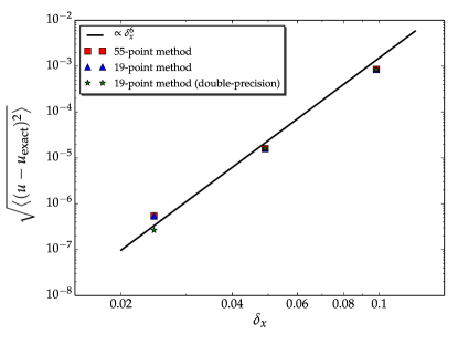
Figure 5: The root mean square of the point-by-point difference between a snapshot and the analytical prediction (Eg. 22) at $t=1.5$ for both 55-point method and 19-point method with single- and double-precision.

Our results are shown in Fig. 5, where we plot the difference between the numerical and analytical solutions as a function of $\delta_{x}$, and make a power-law fit to compare the trend with the expected one for sixth-order finite differences, $\propto\delta_{x}^{6}$, as the resolution is decreased.

With both methods, the measured deviation from the analytical solution is very close to the theoretical discretization error, the average change in the deviation when halving the amount of grid points being $2^{5.7}$. Between the two highest resolution cases the wave is becoming too well resolved, and the single grid point deviation is approaching the floating point accuracy, and therefore the powerlaw starts showing hints of breaking down. However, including double-precision, this breakdown is avoided at the highest resolution. These results clearly show a satisfactory accuracy of the finite-difference scheme with respect to the theoretical expectation.

The second test case was a radial kinetic explosion. The spherical symmetry of the test made it possible to check the symmetry of the computational operation within the code, the rate-of-strain tensor, Eq. (3), in particular. The kinetic energy was released in a small volume with a Gaussian profile, directed radially outward from the centre of the computational domain. In spherical coordinates, this initial condition was defined as

$$\mathbf{u}(\mathbf{r})=u_{\mathrm{ampl}}\exp\bigg{(}\frac{(r-r_{\mathrm{shell}})^{2}}{2d_{\mathrm{shell}}^{2}}\bigg{)}\,\mathbf{\hat{e}}_{r},$$ (23)

where $r_{\mathrm{shell}}$ is the radius of the shell at the peak, $u_{\mathrm{ampl}}$ the peak velocity and $d_{\mathrm{shell}}$ the width parameter. The Gaussian profile helped to avoid numerical instabilities due to discontinuous initial conditions. In a $64^{3}$, $128^{3}$- and $256^{3}$-sized grids we kept $u_{\mathrm{ampl}}=1$, $d_{\mathrm{shell}}=0.2$, $r_{\mathrm{shell}}=0.8$, $\rho_{0}=1$ and varied $\mathrm{Re}$ (Fig. 6) by changing the kinematic viscosity values. The tests were performed with both the 55-point and the 19-point method.

We measure the degree of spherical symmetry on a Cartesian grid by comparing the values of the quantities along 7-directional axes with each other. Three were the $x$-, $y$-, $z$-axes and four diagonals which went from all corners to their opposites. As we could not match the coordinates of Cartesian and the diagonal axes point by point, we integrated the sum of values of each axis $\big{(}\sum\rho\big{)}_{i}$ and $\big{(}\sum|u|\big{)}_{i}$. In the ideal spherically symmetric case, the results for all axes should be the same, therefore we estimated the relative errors between axes by taking standard deviations $\Delta\big{(}\sum\rho\big{)}$ and $\Delta\big{(}\sum|u|\big{)}$. The results are shown in Fig. 6 for the 19-point stencil method. $\Delta\big{(}\sum|u|\big{)}$ is largest for the smallest Reynolds numbers within a certain set with the same resolution. There is a strong decrease when the Reynolds number is increased, and at the highest Reynolds numbers investigated, the difference between the diagonal and off-diagonal elements no longer changes for the highest resolution cases. This is as expected, as the numerical solution is more likely to deviate from the analytic one at small Reynolds numbers where the viscous effects are stronger. For the lowest resolution case no convergence is seen, indicating that this test is too demanding to be performed with that grid spacing. There is a weak, but opposite, trend in $\Delta\big{(}\sum\rho\big{)}$. This is likely to be due to the fact that the decrease of viscosity enhances the effects of the non-conservative nature of the discretized equations. As the 55-point stencil method produces results that practically coincide with the 19-point method, the results are shown in Fig. 6 only for the 19-point method. This test shows that we can satisfactorily re-produce spherically symmetric structures with the numerical scheme.

The third test case explored is a typical forced non-helical turbulence setup. We switch on the external force term in the momentum equation, and use a non-helical forcing function, that can be expressed as

$$\mathbf{f}(\mathbf{x},t)=\mathrm{Re}\bigg{\{}N\mathbf{f}_{\mathbf{k}(t)}\exp\big{(}i\mathbf{k}(t)\cdot\mathbf{x}+i\phi(t)\big{)}\bigg{\}},$$ (24)

where

$$N=f_{0}c_{s}\sqrt{\frac{|\mathbf{k}|c_{s}}{\delta t}}\quad\mathrm{and}\quad\mathbf{f}_{\mathbf{k}(t)}=\frac{\mathbf{k}\times\mathbf{e}}{\sqrt{|\mathbf{k}|^{2}-(\mathbf{k}\cdot\mathbf{e})^{2}}}.$$ (25)

Here $f_{0}$ scales the magnitude of the forcing and $\mathbf{e}$ is an arbitrary unit vector perpendicular to forcing wave vector $\mathbf{k}$ [25]. An isotropic set of $\mathbf{k}$-vectors, with $k_{\mathrm{min}}\leq|\mathbf{k}|\leq k_{\mathrm{max}}$, is generated at the beginning of a computational run, from which they are picked randomly at every timestep.

We denote the mean value of the set of vectors $|\mathbf{k}|$ as $k_{f}$, and chose sets with $k_{f}=1.53$, $2.23$, $3.13$, $4.12$ and $10.0$. With the default domain size $(2\pi,2\pi,2\pi)$ the box size corresponds to $k=1$. We performed the forcing tests using the 19-point stencil method with a $256^{3}$ grid, with $\nu=1.4\cdot 10^{-4}$, which was the lowest viscosity still stable with this resolution.

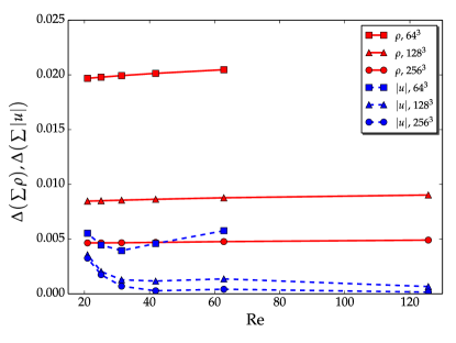
Figure 6: Relative directional errors of $\sum\rho$ and $\sum|u|$ at the end of the explosion tests.

The results of the forced turbulence test are shown as spectra in Fig. 7, which describe the relative distribution of turbulent energy for different wavenumbers $k$. The peak of turbulent energy was situated at the wavenumber of the forcing $k_{f}$ and cascaded into smaller scales or higher wavenumbers. In addition, the spectra show that turbulence behaves isotropically. Following the turbulence theory of Kolmogorov the kinetic energy is expected to scale as $E(k)\propto\sim k^{-5/3}$. However, the inertial range of the turbulence, where the energy distribution follows well the Kolmogorov theory, is quite limited at the Reynolds numbers achievable with the current resolution and viscosity scheme. To increase the effective Reynolds numbers, the implementation of dynamic numerical diffusion schemes, such as shock and hyperviscosities [26] would be needed. However, they are special features which are not relevant to the focus of this study.

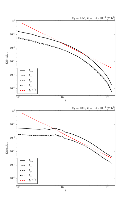
Figure 7: Normalized power spectra of saturated forced turbulence with $k_{f}\sim 1.53$ (top) and $k_{f}\sim 10.0$ (bottom).

7 Discussion and Conclusions

We have implemented two methods based on 19-point and 55-point stencils for simulating compressible fluids on GPUs using third-order Runge-Kutta integration and sixth-order finite differences. Our study is meant as a proof of concept for further developments with multi-GPU systems. The physical problem currently solved for is that of isothermal compressible hydrodynamics.

We show that integration kernels, which operate on 55-point stencils and where each stencil point holds several variables, three-dimensional cache blocking is inefficient because of the limited amount of shared memory available on current GPUs. While the performance of these kernels can be improved with further optimizations, the latencies caused by arithmetic and memory operations are difficult to hide with occupancy without introducing redundant global memory fetches. Using instruction-level-parallelism to hide latencies is similarly problematic, since large amounts of data are required to be cache resident when processing several grid points at once.

We propose a reformulation of the problem, which can be used to improve the performance of the 55-point method by updating the simulation grid in two passes using 19-point stencils. Our results show that the increased occupancy and simpler memory access pattern in our 19-point method outweighs the penalty of performing additional memory transactions.

Moreover, we show that the difference in accuracy of our 19-point and 55-point methods is minimal. Other studies have shown that it is possible to achieve the bandwidth-bound limit in stencil computation [17] [18] [19], which we also achieve with our 19-point implementation.

We report the speedup of $1.7\times$ and $3.6\times$ between a 24 CPU core node and a single GPU with the 55-point and the 19-point methods, respectively. Between a 12-core CPU and a GPU, the corresponding speedups are $3.3\times$ and $6.8\times$. We consider this as a success as typical supercomputer nodes have at least two GPUs, while the most recent offerings of NVIDIA (DGX-1) have up to eight GPUs per node. Although the final outcome of the efforts depends crucially on how well the code scales to multiple GPUs, the current performance is in our view clearly worth the invested time and effort.

We devote the rest of this section for explaining our design decisions and discussing the lessons learnt for future development. There are at least three ways to reduce the cache requirements in order to improve latency-hiding in the 55-point method. First, smaller thread blocks can be used, which require fewer grid points to be cache-resident. However, since the size of the halo stays the same, this approach increases the ratio of memory transfers required for updating a grid point. In a $128^{3}$-sized grid, we reached the update rate of only $85$ million points per second using $(32,4,1)$-sized thread blocks which updated $128$ points per thread and alternatively the update rate of $72$ million points per second with $(4,4,4)$-sized blocks updated $16$ points per thread.

Second, part of the grid points can be stored into local memory while using 2.5-dimensional cache blocking. However, this in turn complicates the program when using 55-point stencils and introduces a large number of redundant fetches from the on-device memory, since only the grid points stored in registers within a warp can be shared with the shuffle instruction. For this reason, we did not explore this approach further.

Finally, the integration kernel can be decomposed into a number of kernels, which use a smaller amount of resources than the initial kernel. As we show with our 19-point method, this optimization technique can be used to transform a latency-bound kernel into a number of kernels, which exhibit higher occupancy. Instead of decomposing the integration kernel of the 55-point method with respect to each dimension, we chose to solve the gradient of divergence separately, which in turn allowed us to use smaller stencils and 2.5-dimensional blocking efficiently, resulting in two bandwidth-bound kernels.

However, the exact speedup gained from kernel decomposition is difficult to predict. If we assume that the time spent on computation in the initial kernel is negligible and that we achieve high enough occupancy with the decomposed kernels to be bandwidth-bound, we can approximate the potential maximum speedup of kernel decomposition with the following equations.

Let $BW_{\mathrm{max}}$ be the maximum effective bandwidth and $BW_{\mathrm{initial}}$ the bandwidth achieved with the latency-bound kernel. Additionally, let $M_{\mathrm{initial}}$ be the number of bytes transferred by the initial kernel and $M_{i}$, where $i\in N$, be the number of bytes transferred by the $i$th kernel of $N$ decomposed kernels.

With these definitions, we can write the time spent on transferring data in the initial kernel and the time spent on transferring data in the decomposed kernels as

$$T_{\mathrm{initial}}=\frac{M_{\mathrm{initial}}}{BW_{\mathrm{initial}}}\ ,\quad T_{\mathrm{decomposed}}=\sum_{i=1}^{N}\frac{M_{i}}{BW_{\mathrm{max}}}\\$$ (26)

Furthermore, we can now write the theoretical maximum speedup as

$$\frac{T_{\mathrm{initial}}}{T_{\mathrm{decomposed}}} =\frac{M_{\mathrm{initial}}}{M_{1}+M_{2}+...+M_{n}}\cdot\frac{BW_{\mathrm{max}}}{BW_{\mathrm{initial}}}\ .$$ (27)

However, both our implementations perform more than the optimal amount of memory transaction to update the simulation grid. Since we store the grid as a structure of arrays and Kepler architecture GPUs service memory transactions from global memory and L2 cache in segments of $32$ bytes, memory bandwidth is wasted on transferring irrelevant bytes when fetching data to the halos on the left and right side of the shared memory block in the $x$-axis. For $R=3$ and using floating-point precision, one such memory transaction wastes bandwidth on transferring $24$ additional bytes. By using an array of structures to store the grid, we would expect a reduction of $25.0\%$ and $3.4\%$ in the number of transactions used to read data with our 55-point and the first half of the 19-point methods, respectively.

In addition, shared memory and memory bandwidth is wasted in our implementation of 55-point method, since we fetch $(\tau_{x}+2R)\times(\tau_{y}+2R)\times(\tau_{z}+2R)$ grid points into shared memory during the initial update even when some of the data is used by only one thread, or none at all. We chose this approach for its simplicity and to avoid branching execution paths in the integration kernel. The optimal size for the shared memory block when using 55-point stencils is hard to formulate, but with a numerical test we found that when $\tau_{x}=\tau_{y}=\tau_{z}=8$ and $R=3$ we use approximately $34\%$ more shared memory with our 55-point method than the amount required for storing only those grid points, which are used by more than one thread. However, we do not know if using less shared memory would increase performance, as in addition to introducing branching to the algorithm, all grid points except the $R^{3}$-sized corners of the shared memory block fall on a memory segment, which is serviced from global memory or L2 cache with a single memory transaction in both approaches regardless of whether the point is stored in shared memory.

Additionally, our 19-point implementation is not compute-bound. Nguyen et. al [18] suggest, that it is possible to be compute-bound in stencil computation by using temporal blocking, where a thread block updates a block of grid points over several timesteps and therefore larger amount of data in shared memory can be reused. However, they also state that temporal blocking requires a large cache to increase performance in stencil computation where $R$ and the size of a grid point is high [18]. In future work, we are planning to explore this approach as well as storing the grid as an array of structures.

Using single-precision and $256^{3}$-sized grids, we saw a $4\%$ improvement in performance when integrating significantly more grid points per thread than in our optimal solution for $128^{3}$-sized grids. A contributing factor was the following. While increasing the workload per thread reduces the number of thread blocks running on the GPU, with larger grids the number of thread blocks is sufficiently large to saturate the GPU with work even when integrating a much larger number of grid points per thread. Solving more grid points per thread increases the reuse factor, which in turn reduces the relative number of global memory fetches needed to integrate a grid point.

While the focus of this work was to accelerate integration using single-precision, we showed that the 19-point method scales well also to double-precision with minimal changes. With the 55-point method, we show that three-dimensional cache blocking becomes less efficient if the data required to integrate a grid point is further increased. Whether further decomposition could improve the performance over our current best solution is a matter of future research. Our tests without the rate-of-strain tensor, $\mathbf{S}$, indicate that the performance of the first half of the 19-point method can potentially be improved by increasing occupancy of the kernel by reducing the requirements for shared memory and registers, which in turn pushes the bandwidth achieved closer to the hardware maximum. However, in order to avoid introducing a large number of additional global memory fetches, as much of the data used for integrating a grid point should be retained in caches until the data is no longer needed.

Also one possible way to reduce shared memory requirements is to decouple the computation with the velocity components and solve the results with respect to one axis at a time. Instead of defining four arrays in shared memory as in the current kernel implementation, we could limit their number to two. In order to improve latency hiding, we could also interleave compute and memory instructions by using a technique called Ping-Pong buffering, where the data is being processed in the ’Ping’ buffer while new data is being fetched into the ’Pong’ buffer. However, a thorough investigation is required to determine whether these approaches can be used to increase the performance of our solver.

We are also planning to extend our implementations to support the full MHD equations. These equations would require additional arrays to be stored in global memory, such as the thermal energy and magnetic fields of the fluid. Since the addition of these new arrays increase the size of a grid point, special care must be taken in order to avoid using large amounts of shared memory. With a single-pass approach, such as our 55-point method, we would expect the occupancy to degrade further if more data is required to be cache-resident during an integration step. Thus, we would expect kernel decomposition to provide speedups also with the full MHD equations, since less data need to be stored in caches at a time in a multi-pass approach.

On the other hand, the latest GPU architectures geared towards scientific computing employ larger caches. For example, a Tesla K80 contains $114688$ bytes of shared memory. In our current 55-point implementation, this would allow two $(8,8,8)$-sized thread blocks to be multithreaded on a SIMD processor instead of only one on a Tesla K40t. However, we did not have access to a Tesla K80 and do not know if the increased occupancy is high enough to hide the latencies in our 55-point method and to outperform our 19-point method.

Additionally, a natural follow-up to our implementations is to extend them to work with multi-node GPUs. We expect inter-node communication to become the bottleneck, because of the comparably slow PCIe bus and communication required for solving boundary conditions. However, an important benefit of a multi-node implementation is that it would allow us to handle larger grids than the current maximum of $512^{3}$ on a Tesla K40t.

Appendix A

The reformulation of the Navier-Stokes equations for the 19-point method is done as follows. For the intermediate result holds that

$$\widetilde{\mathbf{u}}^{(s+1)} =\alpha^{(s)}\widetilde{\mathbf{u}}^{(s)}+\delta_{t}\frac{\partial}{\partial t}\mathbf{u}^{(s)}$$

$$=\alpha^{(s)}\widetilde{\mathbf{u}}^{(s)}+\delta_{t}\biggl{[}-({\mathbf{u}}^{(s)}\cdot\nabla){\mathbf{u}}^{(s)}-c_{s}^{2}\nabla\ln\rho^{(s)}$$

$$+\nu\bigg{(}\nabla^{2}\mathbf{u}^{(s)}+\frac{1}{3}\nabla(\nabla\cdot\mathbf{u}^{(s)})+2\mathbf{S}\cdot\nabla\ln\rho^{(s)}\biggr{)}\biggr{]}$$

$$=\alpha^{(s)}\widetilde{\mathbf{u}}^{(s)}+\delta_{t}\biggl{[}-({\mathbf{u}}^{(s)}\cdot\nabla){\mathbf{u}}^{(s)}-c_{s}^{2}\nabla\ln\rho^{(s)}$$

$$+\nu\bigg{(}\nabla^{2}\mathbf{u}^{(s)}+2\mathbf{S}\cdot\nabla\ln\rho^{(s)}\biggr{)}\biggr{]}+\delta_{t}\frac{\nu}{3}\nabla(\nabla\cdot\mathbf{u}^{(s)})\ .$$

When we set

$$\widetilde{\mathbf{u}}_{partial}^{(s+1)} =\alpha^{(s)}\widetilde{\mathbf{u}}^{(s)}+\delta_{t}\biggl{[}-({\mathbf{u}}^{(s)}\cdot\nabla){\mathbf{u}}^{(s)}-c_{s}^{2}\nabla\ln\rho^{(s)}$$

$$+\nu\bigg{(}\nabla^{2}\mathbf{u}^{(s)}+2\mathbf{S}\cdot\nabla\ln\rho^{(s)}\biggr{)}\biggr{]}\ ,$$

it follows that

$$\widetilde{\mathbf{u}}^{(s+1)}=\widetilde{\mathbf{u}}_{partial}^{(s+1)}+\delta_{t}\frac{\nu}{3}\nabla(\nabla\cdot\mathbf{u}^{(s)})\ .$$

Likewise for the final result

$$\mathbf{u}^{(s+1)} =\mathbf{u}^{(s)}+\beta^{(s)}\widetilde{\mathbf{u}}^{(s+1)}$$

$$=\mathbf{u}^{(s)}+\beta^{(s)}\biggl{(}\widetilde{\mathbf{u}}_{partial}^{(s+1)}+\delta_{t}\frac{\nu}{3}\nabla(\nabla\cdot\mathbf{u}^{(s)})\biggr{)}$$

$$=\mathbf{u}^{(s)}+\beta^{(s)}\widetilde{\mathbf{u}}_{partial}^{(s+1)}+\beta^{(s)}\delta_{t}\frac{\nu}{3}\nabla(\nabla\cdot\mathbf{u}^{(s)})\ .$$

When

$$\mathbf{u}_{partial}^{(s+1)}=\mathbf{u}^{(s)}+\beta^{(s)}\widetilde{\mathbf{u}}_{partial}^{(s+1)}\ ,$$

it follows that

$$\mathbf{u}^{(s+1)}=\mathbf{u}_{partial}^{(s+1)}+\beta^{(s)}\delta_{t}\frac{\nu}{3}\nabla(\nabla\cdot\mathbf{u}^{(s)})\ .$$

References

- [1] A. Brandenburg, in: Antonio Ferriz-Mas, Manuel Núñez (Ed.), Advances in Nonlinear Dynamics, CRC Press, 2003, pp. 269–344. doi:10.1201/9780203493137.ch9.
- [2] E. E. Schneider, B. E. Robertson, CHOLLA: A new massively parallel hydrodynamics code for astrophysical simulation, The Astrophysical Journal Supplement Series 217 (2015) 24. arXiv:1410.4194, doi:10.1088/0067-0049/217/2/24.
- [3] G. L. Bryan, M. L. Norman, B. W. O’Shea, T. Abel, J. H. Wise, M. J. Turk, D. R. Reynolds, D. C. Collins, P. Wang, S. W. Skillman, B. Smith, R. P. Harkness, J. Bordner, J.-h. Kim, M. Kuhlen, H. Xu, N. Goldbaum, C. Hummels, A. G. Kritsuk, E. Tasker, S. Skory, C. M. Simpson, O. Hahn, J. S. Oishi, G. C. So, F. Zhao, R. Cen, Y. Li, Enzo Collaboration, ENZO: An adaptive mesh refinement code for astrophysics, The Astrophysical Journal Supplement 211 (2014) 19. arXiv:1307.2265, doi:10.1088/0067-0049/211/2/19.
- [4] M. K. Griffiths, V. Fedun, R. Erdélyi, A fast MHD code for gravitationally stratified media using graphical processing units: SMAUG, Journal of Astrophysics and Astronomy 36 (2015) 197–223. doi:10.1007/s12036-015-9328-y.
- [5] C. Meng, L. Wang, Z. Cao, X. Ye, L.-L. Feng, Acceleration of a High Order Finite-Difference WENO Scheme for Large-Scale Cosmological Simulations on GPU, IEEE, 2013, pp. 2071–2078. doi:10.1109/IPDPSW.2013.169.
-
[6]
G. Zumbusch,
Vectorized Higher
Order Finite Difference Kernels, Springer Berlin Heidelberg, Berlin,
Heidelberg, 2013, pp. 343–357.
doi:10.1007/978-3-642-36803-5{\_}25.
URL http://dx.doi.org/10.1007/978-3-642-36803-5{_}25 - [7] F. A. Gent, A. Shukurov, G. R. Sarson, A. Fletcher, M. J. Mantere, The supernova-regulated ISM - II. The mean magnetic field, Monthly Notices of the Royal Astronomical Society 430 (2013) L40–L44. arXiv:1206.6784, doi:10.1093/mnrasl/sls042.
- [8] M. J. Käpylä, P. J. Käpylä, N. Olspert, A. Brandenburg, J. Warnecke, B. B. Karak, J. Pelt, Multiple dynamo modes as a mechanism for long-term solar activity variations, Astronomy and Astrophysics 589 (2016) A56. arXiv:1507.05417, doi:10.1051/0004-6361/201527002.
- [9] C.-k. Chan, D. Mitra, A. Brandenburg, Dynamics of saturated energy condensation in two-dimensional turbulence, Physical Review E 85 (3) (2012) 036315. arXiv:1109.6937, doi:10.1103/PhysRevE.85.036315.
- [10] P. Charbonneau, Solar dynamo theory, Annual Review of Astronomy & Astrophysics 52 (2014) 251–290. doi:10.1146/annurev-astro-081913-040012.
- [11] B. G. Elmegreen, J. Scalo, Interstellar turbulence I: Observations and processes, Annual Review of Astronomy & Astrophysics 42 (2004) 211–273. arXiv:astro-ph/0404451, doi:10.1146/annurev.astro.41.011802.094859.
- [12] C. F. McKee, E. C. Ostriker, Theory of star formation, Annual Review of Astronomy & Astrophysics 45 (2007) 565–687. arXiv:0707.3514, doi:10.1146/annurev.astro.45.051806.110602.
- [13] NORDITA, The Pencil Code: A High-Order MPI Code for MHD Turbulence. User’s and Reference Manual, [Online]. Available: http://pencil-code.nordita.org/doc/manual.pdf. Referenced: 2015-08-29. (Aug. 2015).
- [14] V. Volkov, J. W. Demmel, Benchmarking GPUs to tune dense linear algebra, in: Proceedings of the 2008 ACM/IEEE Conference on Supercomputing, IEEE Press, Piscataway, NJ, USA, 2008, pp. 1–11.
- [15] D. A. Patterson, J. L. Hennessy, Computer Organization and Design: The Hardware/Software Interface, 5th Edition, Morgan Kaufmann Publishers, Burlington, MA, USA, 2013.
- [16] J. L. Hennessy, D. A. Patterson, Computer Architecture: A Quantitative Approach, 5th Edition, Morgan Kaufmann Publishers, Burlington, MA, USA, 2011.
- [17] P. Micikevicius, 3D finite difference computation on GPUs using CUDA, in: Proceedings of 2nd Workshop on General Purpose Processing on Graphics Processing Units, ACM, New York, NY, USA, 2009, pp. 79–84.
- [18] A. Nguyen, N. Satish, J. Chhugani, C. Kim, P. Dubey, 3.5D blocking optimization for stencil computations on modern CPUs and GPUs, in: Proceedings of the 2010 ACM/IEEE International Conference for High Performance Computing, Networking, Storage and Analysis, IEEE Computer Society, Washington, DC, USA, 2010, pp. 1–13.
- [19] Y. Zhang, F. Mueller, Auto-generation and auto-tuning of 3D stencil codes on GPU clusters, in: Proceedings of the Tenth International Symposium on Code Generation and Optimization, ACM, New York, NY, USA, 2012, pp. 155–164.
- [20] M. Giles, E. László, I. Reguly, J. Appleyard, J. Demouth, GPU implementation of finite difference solvers, in: Proceedings of the 7th Workshop on High Performance Computational Finance, IEEE Press, Piscataway, NJ, USA, 2014, pp. 1–8.
- [21] A. Vizitiu, L. Itu, C. Nita, C. Suciu, Optimized three-dimensional stencil computation on Fermi and Kepler GPUs, in: High Performance Extreme Computing Conference (HPEC), 2014 IEEE, 2014, pp. 1–6. doi:10.1109/HPEC.2014.7040968.
-
[22]
R. de la Cruz, M. Araya-Polo,
Algorithm 942: Semi-stencil, ACM
Trans. Math. Softw. 40 (3) (2014) 23:1–23:39.
doi:10.1145/2591006.
URL http://doi.acm.org/10.1145/2591006 -
[23]
S. Cygert, D. Kikoła, J. Porter-Sobieraj, J. Sikorski, M. Słodkowski,
Using GPUs for
parallel stencil computations in relativistic hydrodynamic simulation, in:
Parallel Processing and Applied Mathematics, Vol. 8384 of Lecture Notes in
Computer Science, Springer Berlin Heidelberg, 2014, pp. 500–509.
doi:10.1007/978-3-642-55224-3{\_}47.
URL http://dx.doi.org/10.1007/978-3-642-55224-3{_}47 - [24] NVIDIA, CUDA C Best Practices Guide, [Online]. Available: http://docs.nvidia.com/cuda/cuda-c-best-practices-guide/. Referenced: 2015-08-31 (Mar. 2015).
- [25] A. Brandenburg, The inverse cascade and nonlinear alpha-effect in simulations of isotropic helical hydromagnetic turbulence, The Astrophysical Journal 550 (2001) 824–840. arXiv:astro-ph/0006186, doi:10.1086/319783.
- [26] S. E. Caunt, M. J. Korpi, A 3D MHD model of astrophysical flows: Algorithms, tests and parallelisation, Astronomy and Astrophysics 369 (2001) 706–728. arXiv:astro-ph/0102068, doi:10.1051/0004-6361:20010157.