Fermionic currents in AdS spacetime with compact dimensions

Abstract

We derive a closed expression for the vacuum expectation value (VEV) of the fermionic current density in a $(D+1)$-dimensional locally AdS spacetime with an arbitrary number of toroidally compactified Poincaré spatial dimensions and in the presence of a constant gauge field. The latter can be formally interpreted in terms of a magnetic flux treading the compact dimensions. In the compact subspace, the field operator obeys quasiperiodicity conditions with arbitrary phases. The VEV of the charge density is zero and the current density has nonzero components along the compact dimensions only. They are periodic functions of the magnetic flux with the period equal to the flux quantum and tend to zero on the AdS boundary. Near the horizon, the effect of the background gravitational field is small and the leading term in the corresponding asymptotic expansion coincides with the VEV for a massless field in the locally Minkowski bulk. Unlike the Minkowskian case, in the system consisting an equal number of fermionic and scalar degrees of freedom, with same masses, charges and phases in the periodicity conditions, the total current density does not vanish. In these systems, the leading divergences in the scalar and fermionic contributions on the horizon are canceled and, as a consequence of that, the charge flux, integrated over the coordinate perpendicular to the AdS boundary, becomes finite. We show that in odd spacetime dimensions the fermionic fields realizing two inequivalent representations of the Clifford algebra and having equal phases in the periodicity conditions give the same contribution to the VEV of the current density. Combining the contributions from these fields, the current density in odd-dimensional $C$-,$P$- and $T$-symmetric models are obtained. As an application, we consider the ground state current density in curved carbon nanotubes described in terms of a (2+1)-dimensional effective Dirac model.

PACS numbers: 04.62.+v, 03.70.+k, 98.80.-k, 61.46.Fg

1 Introduction

In a number of physical problems one needs to consider the model in background of manifolds with compact subspaces. The presence of extra compact dimensions is an inherent feature of fundamental theories unifying physical interactions, like Kaluza-Klein theories, supergravity and string theories. The compact spatial dimensions also appear in the low-energy effective description of some condensed matter systems. Examples for the latter are the cylindrical and toroidal carbon nanotubes and topological insulators.

In quantum field theory, the periodicity conditions imposed along the compact dimensions modify the spectrum of the zero-point fluctuations of quantum fields. As a consequence of that, the vacuum expectation values (VEVs) of physical quantities are shifted by an amount depending on the geometry of the compact subspace. This general phenomenon, induced by the nontrivial topology, is the analog of the Casimir effect (for reviews see Ref. [1]) where the change in the spectrum of the vacuum fluctuations is caused by the presence of boundaries (conductors, dielectrics, branes in braneworld scenarios, etc.). It is known as the topological Casimir effect and has been investigated for different fields, bulk geometries and topologies. The corresponding vacuum energy depends on the lengths of the compact dimensions and the topological Casimir effect has been considered as a stabilization mechanism for the moduli fields related to extra dimensions. In addition, the vacuum energy induced by the compactification of spatial dimensions can serve as a model for the dark energy driving the accelerated expansion of the universe at a recent epoch [2].

For charged quantum fields, important characteristics for a given state are the expectation values of the charge and current densities. In the present paper we investigate the VEV of the current density for a massive fermionic field in the background of a locally anti-de Sitter (AdS) spacetime with an arbitrary number of toroidally compactified spatial dimensions (for a discussion of physical effects in models with toroidal dimensions, see for instance, Ref. [3]). The corresponding problem for a scalar field with general coupling to the Ricci scalar has been previously considered in Ref. [4] (see also Refs. [5, 6] for additional effects induced by the presence of branes). Both the zero and finite temperature expectation values of the current density for charged scalar and fermionic fields in the background of flat spacetime with toral dimensions were investigated in Refs. [7, 8]. The results were applied to the electronic subsystem of cylindrical and toroidal carbon nanotubes described in terms of a $(2+1)$-dimensional effective field theory. The vacuum current densities for charged scalar and Dirac spinor fields in de Sitter spacetime with toroidally compact spatial dimensions are considered in Ref. [9]. The influence of boundaries on the vacuum currents in topologically nontrivial spaces are studied in Refs. [10, 11, 12] for scalar and fermionic fields. The effects of nontrivial topology induced by the compactification of a cosmic string along its axis have been discussed in Ref. [13]. The vacuum energy and the VEV of the energy-momentum tensor in AdS spacetime with compact subspaces were investigated in Ref. [14].

Our choice of AdS spacetime as the background geometry is motivated by its importance in several recent developments of quantum field theory, gravity and condensed matter physics. The early interest to AdS spacetime as a bulk geometry in quantum field theory was motivated by principal questions of the quantization procedure on curved backgrounds. Because of the maximal symmetry of AdS spacetime, this procedure can be realized explicitly. Compared to the case of the Minkowski bulk, here principally new features arise related to the lack of global hyperbolicity and the presence of both regular and irregular modes. The main reason of the lack of hyperbolicity is that the AdS spacetime possesses a timelike boundary at spatial infinity through which the information may be lost or gained in finite coordinate time [15]. As a consequence, boundary conditions should be imposed at infinity to ensure a consistent quantum field theory. The natural appearance of AdS spacetime as a ground state in certain supergravity theories and also as the near horizon geometry of the extremal black holes and domain walls has stimulated further interest in quantum fields propagating on that background. Moreover, the AdS spacetime is a constant negative curvature manifold and the corresponding length scale can be used for the regularization of infrared divergences in interacting quantum field theories [16]. The dimension of the AdS isometry group is the same as that of the Poincaré group and the regularization is realized without reducing the symmetries.

The renewed interest in physical models on AdS bulk is closely related to two rapidly developing fields in theoretical physics: the gauge/gravity duality and the braneworld scenario. The AdS spacetime played a crucial role in the original formulations of both these concepts in the form of the AdS/CFT correspondence [17] and the Randall-Sundrum type braneworlds [18]. The AdS/CFT correspondence (for reviews see Ref. [19]) is a type of holographic duality between two theories living in spacetimes with different dimensions: string theories or supergravity in the AdS bulk from one side and a conformal field theory localized on the AdS boundary from another. Among many interesting consequences, this duality opens an important opportunity to study quantum field theoretical effects in strongly coupled regime using a classical gravitational theory. It has also been used for the investigation of non-equilibrium phenomena in strongly coupled condensed matter systems. One of the applications is the holographic model for superconductors suggested in Ref. [20] (for a recent discussion with references, see e.g., Ref. [21]). In this model, the quantum physics of strongly correlated condensed matter system is mapped to the gravitational dynamics with black holes in one higher dimension.

The braneworld scenario (see Ref. [22] for a review) provides an interesting alternative to the standard Kaluza-Klein compactification of extra dimensions. It uses the concept of brane as a submanifold embedded in a higher dimensional spacetime, on which the standard model fields are confined. Braneworlds naturally appear in the string/M-theory context and provide interesting possibilities to solve or to address from a different point of view various problems in cosmology and particle physics. In the model introduced by Randall and Sundrum the background geometry consists of two parallel branes, with positive and negative tensions, embedded in a five dimensional AdS bulk [18]. The fifth coordinate is compactified on orbofold and the branes are located at the two fixed points. The large hierarchy between the Planck and electroweak mass scales is generated by the large physical volume of the extra dimension. From the point of view of embedding the corresponding models into a more fundamental theory, such as string/M-theory, one may expect the presence of additional extra dimensions compactified on an internal manifold. Here we will consider a simple case of toroidal compactification of spatial dimensions in Poincaré coordinates.

The plan of the paper is as follows. In the next section the problem is formulated and the complete set of fermionic modes is presented. By using these modes, in Section 3, we evaluate the VEV of the fermionic current density along compact dimensions. The asymptotics near the AdS boundary and near the horizon are investigated and limiting cases are discussed. In Section 4, we consider the current density in $C$-, $P$-, $T$-symmetric odd-dimensional models. The corresponding VEV is obtained by combining the results for two fermionic fields realizing the irreducible representations of the Clifford algebra. Applications are given to graphene made structures realizing the geometry under consideration. The main results of the paper are summarized in Section 5. In Appendix A we consider an alternative representation of the Dirac matrices allowing for the separation of the equations for the upper and lower components of the fermionic mode functions in Poincaré coordinates. The main steps for the evaluation of the mode-sum for the current density are presented in Appendix B.

2 Problem setup and the fermionic modes

The dynamics of a fermionic field $\psi(x)$ in a $(D+1)$-dimensional curved background with a metric tensor $g_{\mu\nu}(x)$ and in the presence of an abelian gauge field $A_{\mu}(x)$ is described by the Dirac equation

$$i\gamma^{\mu}D_{\mu}\psi-m\psi=0,$$ (2.1)

with the gauge extended covariant derivative $D_{\mu}=\partial_{\mu}+\Gamma_{\mu}+ieA_{\mu}$. Here, $\Gamma_{\mu}$ is the spin connection and the curved spacetime Dirac matrices $\gamma^{\mu}$ are expressed in terms of the corresponding flat spacetime matrices $\gamma^{(b)}$ as $\gamma^{\mu}=e_{(b)}^{\mu}\gamma^{(b)}$, where $e_{(b)}^{\mu}$ are the tetrad fields. In this and in the next sections we consider a fermionic field realizing the irreducible representation of the Clifford algebra. In $(D+1)$-dimensional spacetime the corresponding Dirac matrices are $N\times N$ matrices, where $N=2^{[(D+1)/2]}$ and $[x]$ is the integer part of $x$ (for the Dirac matrices in an arbitrary number of the spacetime dimension see, for example, Ref. [23]). In even-dimensional spacetimes the irreducible representation is unique up to a similarity transformation, whereas in odd-dimensional spacetimes there are two inequivalent irreducible representations (see Section 4 below).

As a background geometry we consider a locally AdS spacetime with the line element

$$ds^{2}=e^{-2y/a}\eta_{ik}dx^{i}dx^{k}-dy^{2},$$ (2.2)

where $a$ is the curvature radius, $i,k=0,1,\ldots,D-1$ and $\eta_{ik}=\mathrm{diag}(1,-1,\ldots,-1)$. We assume that the subspace covered by the coordinates $(x^{p+1},\ldots,x^{D-1})$ is compactified to a $q$-dimensional torus $T^{q}$ with $q=D-p-1$. The length of the $l$th compact dimension will be denoted by $L_{l}$, $0\leqslant x^{l}\leqslant L_{l}$, $l=p+1,\ldots,D-1$. The subspace $(x^{1},\ldots,x^{p})$ has trivial topology $R^{p}$ with $-\infty<x^{l}<+\infty$, $l=1,\ldots,p$, and for the coordinate $y$ one has $-\infty<y<+\infty$. Note that the compactification to the torus does not change the local AdS geometry with the scalar curvature $R=-D(D+1)/a^{2}$. In terms of a new spatial coordinate $z=ae^{y/a}$, $0\leqslant z<\infty$, the line element is presented in a conformally-flat form

$$ds^{2}=(a/z)^{2}(\eta_{ik}dx^{i}dx^{k}-dz^{2}).$$ (2.3)

The AdS boundary and horizon correspond to the hypersurfaces $z=0$ and $z=\infty$, respectively. Note that $L_{l}$ is the coordinate length of the compact dimension. For a given $z$, the proper length is given by $L_{(p)l}=(a/z)L_{l}$. The latter decreases with increasing $z$. In the conformal coordinates $(x^{1},\ldots,x^{D-1},x^{D}=z)$, the tetrad fields can be chosen as $e_{(b)}^{\mu}=(z/a)\delta_{b}^{\mu}$. For the corresponding components of the spin connection one gets $\Gamma_{k}=\eta_{kl}\gamma^{(D)}\gamma^{(l)}/(2z)$ for $k=0,\ldots,D-1$, and $\Gamma_{D}=0$.

In the presence of compact dimensions, the field equation (2.1) should be supplemented by the periodicity conditions on the field operator along those directions. Here, we will impose quasiperiodicity conditions

$$\psi(t,x^{1},\ldots,x^{l}+L_{l},\ldots,x^{D})=e^{i\alpha_{l}}\psi(t,x^{1},\ldots,x^{l},\ldots,x^{D}),$$ (2.4)

with constant phases $\alpha_{l}$, $l=p+1,\ldots,D-1$. The special cases $\alpha_{l}=0$ and $\alpha_{l}=\pi$ correspond to untwisted and twisted fermionic fields, most frequently discussed in the literature. For the gauge field we will consider the simplest configuration $A_{\mu}=\mathrm{const}$. Though the corresponding field tensor vanishes, the nontrivial topology of the background spacetime gives rise the Aharonov-Bohm like effect on the VEVs of physical observables. For this special field configuration, the gauge field can be removed from the field equation by the gauge transformation

$$\psi=\psi^{\prime}e^{-ie\chi},\;A_{\mu}=A_{\mu}^{\prime}+\partial_{\mu}\chi,$$ (2.5)

with the function $\chi=A_{\mu}x^{\mu}$. In the new gauge $A_{\mu}^{\prime}=0$. However, the gauge potential does not disappear from the problem completely. The gauge transformation of the field operator modifies the corresponding periodicity conditions. For the new field it takes the form

$$\psi^{\prime}(t,x^{1},\ldots,x^{l}+L_{l},\ldots,x^{D})=e^{i\tilde{\alpha_{l}}}\psi^{\prime}(t,x^{1},\ldots,x^{l},\ldots,x^{D}),$$ (2.6)

with the new phases

$$\tilde{\alpha_{l}}=\alpha_{l}+eA_{l}L_{l}.$$ (2.7)

The VEVs of physical observables will depend on the set $\{\alpha_{l},A_{l}\}$ in the form of the combination (2.7). Under the gauge transformation (2.5) with $\chi=b_{\mu}x^{\mu}$ and constant $b_{\mu}$, we obtain a new set $\{\alpha_{l}+eb_{l}L_{l},A_{l}-b_{l}\}$. However, the combination (2.7) remains invariant. Note that the phase shift in Eq. (2.7), induced by the gauge field, can be presented as $eA_{l}L_{l}=-2\pi\Phi_{l}/\Phi_{0}$, where $\Phi_{0}=2\pi/e$ is the flux quantum. The quantity $\Phi_{l}$ can be formally interpreted as the magnetic flux enclosed by the $l$th compact dimension, $\Phi_{l}=-\oint dx^{l}A_{l}$ (no summation over $l$). This flux acquires real physical meaning in models where the spacetime under consideration is embedded in a higher-dimensional manifold as a hypersurface (like branes in braneworld scenario) on which the fermionic field $\psi(x)$ is localized. In what follows we will work in the gauge $(A_{\mu}^{\prime}=0,\psi^{\prime}(x))$ omitting the prime for the fermionic field. In this gauge, in Eq. (2.1) we have $D_{\mu}=\partial_{\mu}+\Gamma_{\mu}$. Of course, the VEVs of physical observables do not depend on the choice of the gauge.

We are interested in the VEV of the fermionic current density $\langle 0|j^{\mu}(x)|0\rangle\equiv\langle j^{\mu}(x)\rangle$ with the operator $j^{\mu}(x)=e\bar{\psi}(x)\gamma^{\mu}\psi(x)$, where $|0\rangle$ stands for the vacuum state and $\bar{\psi}(x)=\psi^{\dagger}\gamma^{(0)}$. The VEV is presented as the coincidence limit

$$\langle j^{\mu}(x)\rangle=-\frac{e}{2}\lim_{x^{\prime}\rightarrow x}\mathrm{Tr}(\gamma^{\mu}S^{(1)}(x,x^{\prime})),$$ (2.8)

with the two-point function $S_{ik}^{(1)}(x,x^{\prime})=\langle 0|[\psi_{i}(x),\bar{\psi}_{k}(x^{\prime})]|0\rangle$ and with $i$, $k$ being spinor indices. Expanding the field operator in terms of a complete set of mode functions $\{\psi_{\beta}^{(+)}(x),\psi_{\beta}^{(-)}(x)\}$ for the Dirac equation and using the anticommutation relations for the annihilation and creation operators, one gets the mode-sum representation

$$\langle j^{\mu}\rangle=\frac{e}{2}\sum_{\beta}\left[\bar{\psi}_{\beta}^{(-)}(x)\gamma^{\mu}\psi_{\beta}^{(-)}(x)-\bar{\psi}_{\beta}^{(+)}(x)\gamma^{\mu}\psi_{\beta}^{(+)}(x)\right].$$ (2.9)

Here, $\beta$ is the set of quantum numbers specifying the fermionic modes and $\sum_{\beta}$ is understood as summation for discrete subset of quantum numbers and integration over the continues ones. Following Ref. [24] (see also [25] for the geometry with a cosmic string perpendicular to the AdS boundary), in the discussion below we will take the Dirac matrices in the representation

$$\gamma^{0}=i\frac{z}{a}\left(\begin{array}[]{cc}0&-1\\ 1&0\end{array}\right),\;\gamma^{l}=i\frac{z}{a}\left(\begin{array}[]{cc}-\sigma_{l}&0\\ 0&\sigma_{l}\end{array}\right),$$ (2.10)

with $l=1,\ldots,D$. The $N/2\times N/2$ matrices $\sigma_{l}$ obey the anticommutation relations $\sigma_{l}\sigma_{k}+\sigma_{k}\sigma_{l}=2\delta_{lk}$. For hermitian $\sigma_{l}$ one has $\gamma^{0\dagger}=\gamma^{0}$ and $\gamma^{l\dagger}=-\gamma^{l}$.

The complete set of the modes for the problem under consideration can be found in the way similar to that used in Ref. [24] for the usual AdS bulk. The positive-energy modes are presented as

$$\psi_{\beta}^{(+)}=C_{\beta}^{(+)}z^{\frac{D+1}{2}}e^{i\mathbf{kx}-i\omega t}\left(\begin{array}[]{c}\widehat{Z}_{-}(\lambda z)w^{(\sigma)}\\ \frac{1}{\omega}\widehat{Z}_{+}(\lambda z)\left(i\lambda+\mathbf{k\sigma}\right)w^{(\sigma)}\end{array}\right),$$ (2.11)

where $0\leqslant\lambda<\infty$, $\omega=\sqrt{\lambda^{2}+k^{2}}$, $\mathbf{kx}=\sum_{l=1}^{D-1}k_{l}x^{l}$, $\mathbf{k\sigma}=\sum_{l=1}^{D-1}k_{l}\sigma_{l}$, and

$$\widehat{Z}_{\pm}(x)=\left(\begin{array}[]{cc}J_{ma\pm 1/2}(x)&0\\ 0&J_{ma\mp 1/2}(x)\end{array}\right),$$ (2.12)

with $J_{\nu}(x)$ being the Bessel function. In Eq. (2.11), $w^{(\sigma)}$, $\sigma=$ $1,\ldots,N/2$, are one-column matrices having $N/2$ rows, with the elements $w_{l}^{(\sigma)}=\delta_{l\sigma}$. For the negative-energy modes we get

$$\psi_{\beta}^{(-)}=C_{\beta}^{(-)}z^{\frac{D+1}{2}}e^{i\mathbf{kx}-i\omega t}\left(\begin{array}[]{c}\frac{1}{\omega}\widehat{Z}_{-}(\lambda z)\left(i\lambda-\mathbf{k\sigma}\right)w^{(\sigma)}\\ \widehat{Z}_{+}(\lambda z)w^{(\sigma)}\end{array}\right).$$ (2.13)

The fermionic states are now specified by the set of quantum numbers $\beta=(\mathbf{k},\lambda,\sigma)$.

The eigenvalues of the momentum components along the compact dimensions are found from the quasiperiodicity conditions (2.6):

$$k_{l}=\frac{2\pi n_{l}+\tilde{\alpha_{l}}}{L_{l}},\;l=p+1,\ldots,D-1,$$ (2.14)

with $n_{l}=0,\pm 1,\pm 2,\ldots$. For the components of the momentum along the noncompact dimensions one has $-\infty<k_{l}<+\infty$, $l=1,\ldots,p$. The coefficients $C_{\beta}^{(\pm)}$ are found from the normalization condition $\int d^{D}x\,(a/z)^{D}\psi_{\beta}^{(\pm)\dagger}\psi_{\beta^{\prime}}^{(\pm)}=\delta_{\beta\beta^{\prime}}$, where $\delta_{\beta\beta^{\prime}}$ is understood as the Kronecker delta for discrete quantum numbers and the Dirac delta function for the continuous ones. From that condition one gets

$$\left|C_{\beta}^{(\pm)}\right|^{2}=\frac{\lambda}{2(2\pi)^{p}V_{q}a^{D}},$$ (2.15)

where $V_{q}=L_{p+1}\cdots L_{D-1}$ is the volume of the compact subspace.

In defining the mode functions (2.11) and (2.13), as a solution of the Bessel equation we have taken the Bessel function of the first kind (see Eq. (2.12)). In the range $ma\geqslant 1/2$ this choice is uniquely dictated by the normalizability condition of the mode functions: for the solution with the Neumann function $Y_{ma\pm 1/2}(x)$ the normalization integral over $z$ diverges at the lower limit $z=0$. For $ma<1/2$ both solutions of the Bessel equation are normalizable and, in general, we can take in Eq. (2.12) the linear combination of the Bessel and Neumann functions. The first one of the coefficients in that linear combination is obtained from the normalization condition, whereas the second one is not uniquely determined. In the case $ma<1/2$, the normalized mode functions are obtained in a way similar to that we have presented above. They are still given by Eqs. (2.11) and (2.13) with the same coefficients $C_{\beta}^{(\pm)}$, where now in Eq. (2.12) we need to make the replacement

$$J_{ma\pm 1/2}(x)\rightarrow\frac{J_{ma\pm 1/2}(x)+B_{\beta}Y_{ma\pm 1/2}(x)}{\sqrt{1+B_{\beta}^{2}}}.$$ (2.16)

Here, the coefficient $B_{\beta}$ (which, in general, depends on quantum numbers) should be specified by an additional boundary condition on the AdS boundary (for a discussion of boundary conditions on fermionic fields in AdS see Refs. [26, 27, 28]). In what follows, for $ma<1/2$ we consider the boundary condition corresponding to $B_{\beta}=0$. It can be seen that this corresponds to the situation where the bag boundary condition is imposed on the fermionic field at $z=\delta>0$ and then the limit $\delta\rightarrow 0$ is taken (for the corresponding procedure in the case of the AdS bulk without compactification see Ref. [24]). This ensures the vanishing of the fermionic currents through the AdS boundary.

3 Fermionic current

By using the mode-sum formula (2.9) with the Dirac matrices (2.10) and the modes (2.11), (2.13), we can see that the VEVs of the charge density and of the components of the current density along noncompact dimensions vanish: $\langle j^{\mu}\rangle=0$, $\mu=0,1,\ldots,p,D$. For the current density along the $l$th compact dimension, $l=p+1,\ldots,D-1$, we find

$$\langle j^{l}\rangle=-\frac{(4\pi)^{-p/2}eNz^{D+2}}{2\Gamma(p/2)V_{q}a^{D+1}}\sum_{\mathbf{n}_{q}}\int_{0}^{\infty}dk_{(p)}\,k_{(p)}^{p-1}\int_{0}^{\infty}d\lambda\,\frac{\lambda k_{l}}{\omega}\left[J_{ma+1/2}^{2}(\lambda z)+J_{ma-1/2}^{2}(\lambda z)\right],$$ (3.1)

where $\mathbf{n}_{q}=(n_{p+1},\ldots,n_{D-1})$, $-\infty<n_{i}<+\infty$, $k_{(p)}^{2}=\sum_{i=1}^{p}k_{i}^{2}$, $\omega^{2}=\lambda^{2}+k_{(p)}^{2}+k_{(q)}^{2}$, and

$$k_{(q)}^{2}=\sum_{i=p+1}^{D-1}k_{i}^{2}=\sum_{i=p+1}^{D-1}\frac{(2\pi n_{i}+\tilde{\alpha}_{i})^{2}}{L_{i}^{2}}.$$ (3.2)

The same expression for the VEV of the current density is obtained in Appendix A by using another representation for the gamma matrices. In the AdS bulk without compactification the VEV of the current density vanishes (for a recent discussion of the finite temperature expectation value see Ref. [29]).

For the further transformation of the current density, we write the VEV in the form

$$\langle j^{l}\rangle=-\frac{(4\pi)^{-p/2}eNz^{D+2}}{2\Gamma(p/2)V_{q}a^{D+1}}\left[\mathcal{I}_{ma}(z)+\mathcal{I}_{ma-1}(z)\right],$$ (3.3)

with the function

$$\mathcal{I}_{\nu}(z)=\sum_{\mathbf{n}_{q}}\int_{0}^{\infty}dk_{(p)}\,k_{(p)}^{p-1}\int_{0}^{\infty}d\lambda\,\frac{\lambda k_{l}}{\omega}J_{\nu+1/2}^{2}(\lambda z).$$ (3.4)

The transformation of this function is presented in Appendix B with the final result given by Eq. (B.5). As a result, for the current density we find

$$\langle j^{l}\rangle=-\frac{eNa^{-D-1}L_{l}}{(2\pi)^{(D+1)/2}}\sum_{n_{l}=1}^{\infty}n_{l}\sin(\tilde{\alpha}_{l}n_{l})\sum_{\mathbf{n}_{q-1}}\,\cos(\tilde{\mathbf{\alpha}}_{q-1}\cdot\mathbf{n}_{q-1})\sum_{j=0,1}q_{ma-j}^{\left(D+1\right)/2}(b_{\mathbf{n}_{q}}),$$ (3.5)

with $\mathbf{n}_{q-1}=(n_{p+1},\ldots,n_{l-1},n_{l+1},\ldots,n_{D-1})$, $\tilde{\mathbf{\alpha}}_{q-1}\cdot\mathbf{n}_{q-1}=\sum_{i=1,\neq l}^{D-1}\tilde{\alpha}_{i}n_{i}$, and

$$b_{\mathbf{n}_{q}}=1+\frac{g_{\mathbf{n}_{q}}^{2}}{2z^{2}},\;g_{\mathbf{n}_{q}}^{2}=\sum_{i=p+1}^{D-1}n_{i}^{2}L_{i}^{2}.$$ (3.6)

Here, the function $q_{ma-j}^{\left(D+1\right)/2}(u)$ is defined by Eq. (B.7) or, equivalently, by the integral representation (B.6). The VEV of the current density for a charged scalar field is also expressed in terms of this function [4].

The VEV of the component of the current density along the compact dimension $x^{l}$ is an odd periodic function of $\tilde{\alpha}_{l}$ and an even periodic function of the remaining phases. In terms of the magnetic fluxes $\Phi_{i}$, the period is equal to the flux quantum $\Phi_{0}$. The current (3.5) determines the charge flux through the spatial hypersurface $x^{l}=\mathrm{const}$. Denoting by $n_{i}^{(l)}$, $n_{i}^{(l)}=\delta_{i}^{l}a/z$, the normal to this hypersurface, for the charge flux one gets (no summation over $l$) $n_{i}^{(l)}\langle j^{i}\rangle=n_{l}^{(l)}\langle j^{l}\rangle$. It depends on the lengths $L_{i}$ and on the coordinate $z$ through the ratio $L_{i}/z$. This ratio is the proper length of the $i$th compact dimension measured by an observer with a fixed $z$, in units of the curvature radius of the background geometry, $L_{i}/z=L_{(p)i}/a$. We could expect this feature from the maximal symmetry of the AdS spacetime. Of course, the current density (3.5) obeys the covariant conservation equation $\partial_{l}(\sqrt{|g|}\langle j^{l}\rangle)=0$ with $\sqrt{|g|}=(a/z)^{D+1}$.

In the model with a single compact dimension $x^{l}$ with the length $L_{l}=L$ and with the phase $\tilde{\alpha}_{l}=\tilde{\alpha}$, the general result (3.5) is reduced to

$$\langle j^{l}\rangle=-\frac{eNa^{-D-1}L}{(2\pi)^{(D+1)/2}}\sum_{n=1}^{\infty}n\sin(\tilde{\alpha}n)\sum_{j=0,1}q_{ma-j}^{\left(D+1\right)/2}\left(1+\frac{n^{2}L^{2}}{2z^{2}}\right).$$ (3.7)

In Fig. 1, for $D=4$ and $ma=1$, we have plotted the corresponding charge flux measured in units of $a^{-D}$, namely, $a^{D}n_{l}^{(l)}\langle j^{l}\rangle$, as a function of the phase $\tilde{\alpha}$ and of the ratio $z/L$. The current density is a periodic function of $\tilde{\alpha}$ with the period $2\pi$. As it will be shown below by asymptotic analysis, the charge flux vanishes on the AdS boundary and diverges on the AdS horizon.

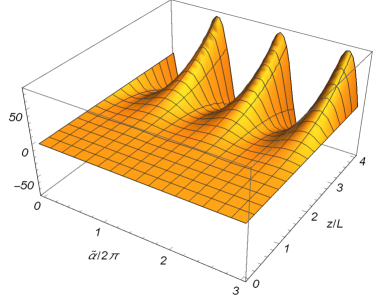
Figure 1: The charge flux along the compact dimension, $a^{D}n_{l}^{(l)}\langle j^{l}\rangle$, in the model with $p=3$, $q=1$ as a function of the phase $\tilde{\alpha}$ and of the ratio $z/L$. For the mass we have taken $ma=1$.

Let us consider some special cases of the general formula (3.5). For a massless field, $m=0$, the expressions for the functions $q_{0}^{\left(D+1\right)/2}(u)$ and $q_{-1}^{\left(D+1\right)/2}(u)$ are most easily found by using the representation (B.6) and the expressions for the functions $I_{\pm 1/2}(x)$. This gives

$$q_{j}^{\left(D+1\right)/2}(u)=\frac{1}{2}\Gamma\left(\frac{D+1}{2}\right)\left[\frac{1}{\left(u-1\right)^{(D+1)/2}}-\frac{(-1)^{j}}{\left(u+1\right)^{(D+1)/2}}\right],$$ (3.8)

for $j=0,-1$. Plugging into Eq. (3.5), for the current density one gets $\langle j^{l}\rangle=(z/a)^{D+1}\langle j^{l}\rangle_{\mathrm{M}}$, where

$$\langle j^{l}\rangle_{\mathrm{M}}=-\frac{e\Gamma((D+1)/2)}{\pi^{(D+1)/2}}NL_{l}\sum_{n_{l}=1}^{\infty}n_{l}\sin(\tilde{\alpha}_{l}n_{l})\sum_{\mathbf{n}_{q-1}}\,\frac{\cos(\tilde{\mathbf{\alpha}}_{q-1}\cdot\mathbf{n}_{q-1})}{g_{\mathbf{n}_{q}}^{D+1}},$$ (3.9)

is the VEV for a massless fermionic field in $(D+1)$-dimensional Minkowski spacetime with spatial topology $R^{p+1}\times T^{q}$. The expression (3.9) is obtained from the more general result from Ref. [8] for a massive fermionic field in the limit $m\rightarrow 0$ (with the replacement $\tilde{\alpha}_{l}\rightarrow-2\pi\tilde{\alpha}_{l}$). Note that, because of the boundary condition we have imposed on the fermionic modes on the AdS boundary, for a massless field the problem under consideration is conformally related to the problem in locally Minkowski spacetime with a boundary at $z=0$ on which the fermionic field obeys the bag boundary condition. The reason why the current density $\langle j^{l}\rangle$ is conformally related to the current density $\langle j^{l}\rangle_{\mathrm{M}}$ in the boundary-free Minkowski case, is that the boundary-induced contribution in the latter problem vanishes for a massless field (see Ref. [10]).

The current density on the Minkowski bulk is obtained in the limit $a\rightarrow\infty$ for fixed $y$. The conformal coordinate $z$ is expanded as $z=a+y+\cdots$. In the integral representation (B.6) for the function $q_{\nu}^{\left(D+1\right)/2}(u)$ the order of the Bessel function is large and we use the corresponding uniform asymptotic expansion. To the leading order, this gives

$$\sum_{j=0,1}q_{ma-j}^{\left(D+1\right)/2}(u)=2m^{(D+1)/2}a^{D+1}\frac{K_{(D+1)/2}(mu)}{u^{(D+1)/2}},$$ (3.10)

with $u=b_{\mathbf{n}_{q}}$ and $K_{\nu}(x)$ being the Macdonald function. Substituting into Eq. (3.5) we get $\lim_{a\rightarrow\infty}\langle j^{l}\rangle=\langle j^{l}\rangle_{\mathrm{M}}$ with the Minkowskian result

$$\langle j^{l}\rangle_{\mathrm{M}}=-\frac{2eNL_{l}m^{(D+1)/2}}{(2\pi)^{(D+1)/2}}\sum_{n_{l}=1}^{\infty}n_{l}\sin(\tilde{\alpha}_{l}n_{l})\sum_{\mathbf{n}_{q-1}}\,\cos(\tilde{\mathbf{\alpha}}_{q-1}\cdot\mathbf{n}_{q-1})\frac{K_{(D+1)/2}(mg_{\mathbf{n}_{q}})}{g_{\mathbf{n}_{q}}^{(D+1)/2}}.$$ (3.11)

The latter coincides with the expression obtained in Ref. [8] (again, with the replacement $\tilde{\alpha}_{l}\rightarrow-2\pi\tilde{\alpha}_{l}$). In Fig. 2, for the model with $D=4$ and with a single compact dimension, we have plotted the ratio of the charge fluxes in locally AdS and Minkowski spacetimes, with the same proper lengths of the compact dimension, as a function of the proper length measured in units of the AdS curvature radius $a$. For the phase in the quasiperiodicity condition along the compact dimension we have taken $\tilde{\alpha}=\pi/2$ and the numbers near the curves correspond to the values of $ma$. As is seen from the graphs, for large values of the proper length the charge flux in the AdS bulk is essentially larger than that for the Minkowski case. As it will be shown below, in the former case the decay of the current density for large values of the proper length goes like a power law, whereas in the Minkowski background and for a massive field the decay is exponential (see Eq. (3.11)).

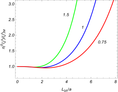
Figure 2: The ratio of the charge fluxes in locally AdS and Minkowski spacetimes, with the same proper lengths of the compact dimension, versus the proper length. The graphs are plotted for $\tilde{\alpha}=\pi/2$ and for different values of $ma$ (numbers near the curves).

Now we turn to the asymptotics of the current density for small and large values of $z$. Near the AdS boundary, $z\rightarrow 0$, the argument of the function $q_{\nu}^{(D+1)/2}(u)$ in Eq. (3.5) is large. By using the corresponding asymptotic from Ref. [4], we can see that the dominant contribution comes from the term $q_{ma-1}^{\left(D+1\right)/2}(b_{\mathbf{n}_{q}})$ and, to the leading order,

$$\langle j^{l}\rangle \approx -\frac{eNL_{l}\Gamma(ma+(D+1)/2)}{\pi^{D/2}a^{D+1}\Gamma(ma+1/2)}z^{D+1+2ma}$$ (3.12)

$$\times\sum_{n_{l}=1}^{\infty}n_{l}\sin(\tilde{\alpha}_{l}n_{l})\sum_{\mathbf{n}_{q-1}}\,\frac{\cos(\tilde{\mathbf{\alpha}}_{q-1}\cdot\mathbf{n}_{q-1})}{g_{\mathbf{n}_{q}}^{D+1+2ma}}.$$

For a massless field this coincides with the exact result. As seen, the current density vanishes on the AdS boundary as $z^{D+1+2ma}$. For a special case $D=4$ with a single compact dimension this has been already demonstrated numerically in figure 1. The large values of $z$ correspond to the near horizon limit. In this limit one has $b_{\mathbf{n}_{q}}-1\ll 1$ and by using the asymptotic

$$q_{\nu}^{\left(D+1\right)/2}(u)\approx\frac{\Gamma\left((D+1)/2\right)}{2\left(u-1\right)^{(D+1)/2}}\left[1-\frac{\nu\left(\nu+1\right)}{D-1}\left(u-1\right)\right],$$ (3.13)

valid for $u-1\ll 1$, to the leading order we find $\langle j^{l}\rangle\approx(z/a)^{D+1}\langle j^{l}\rangle_{\mathrm{M}}$, with $\langle j^{l}\rangle_{\mathrm{M}}$ given by Eq. (3.9). Near the horizon the dominant contribution comes from the fluctuations with small wavelengths, and the effects induced by the curvature and nonzero mass are small.

Let us consider the behavior of the current density in asymptotic regions of the lengths for compact dimensions. If the length of the $l$th compact dimension is much smaller than the other lengths, $L_{l}\ll L_{i}$, $i\neq l$, and $L_{l}\ll z$, the leading contribution comes from the term with $\mathbf{n}_{q-1}=0$ and by using the asymptotic expression for the function $q_{\nu}^{(D+1)/2}(u)$ for the values of the argument close to 1, one finds

$$\langle j^{l}\rangle\approx-\frac{eNL_{l}\Gamma((D+1)/2)}{\pi^{(D+1)/2}\left(aL_{l}/z\right)^{D+1}}\sum_{n_{l}=1}^{\infty}\frac{\sin(\tilde{\alpha}_{l}n_{l})}{n_{l}^{D}}.$$ (3.14)

The contribution to the current density from the terms $\mathbf{n}_{q-1}\neq 0$ is suppressed by the exponential factor $e^{-\sigma_{l}|\mathbf{L}\cdot\mathbf{n}_{q-1}|/L_{l}}$, with $\sigma_{l}=\mathrm{min}(\tilde{\alpha}_{l},2\pi-\tilde{\alpha}_{l})$, $0<\tilde{\alpha}_{l}<2\pi$. Note that Eq. (3.14) coincides with the current density for a massless field in the model with a single compact dimension $x^{l}$.

For large values of the proper length of the $l$th compact dimension compared with the AdS curvature radius one has $L_{(p)l}/a=L_{l}/z\gg 1$ and, hence, $b_{\mathbf{n}_{q}}\gg 1$. By using the asymptotic expression for the function $q_{\nu}^{(D+1)/2}(u)$ for large values of the argument, for the leading order term in the current density one gets the result (3.12). If in addition $L_{l}\gg L_{i}$, $i\neq l$, the contribution from large values of $|n_{i}|$ dominates and the corresponding summations can be replaced by the integration. Two cases should be considered separately. If all the phases $\tilde{\alpha}_{i}$, $i\neq l$, are zero the leading term is given by

$$\langle j^{l}\rangle\approx-\frac{Ne\Gamma(p/2+ma+3/2)}{\pi^{p/2+1}\Gamma(ma+1/2)a^{D+1}V_{q}}\frac{z^{D+2ma+1}}{L_{l}^{p+2ma+1}}\sum_{n_{l}=1}^{\infty}\frac{\sin(\tilde{\alpha}_{l}n_{l})}{n_{l}^{p+2ma+2}}.$$ (3.15)

As is seen, in this case, for a given $z$, the decay of the current density as a function of the proper length $L_{(p)l}$ follow a power law. For a massive field this behavior essentially differs from that for the current density in the Minkowski bulk. In the latter geometry and for a massive field, the current decays exponentially, as $e^{-mL_{l}}$. Provided at least one of the phases $\tilde{\alpha}_{i}$, $i\neq l$, is different from zero, the current density is dominated by the term $n_{l}=1$ and one finds

$$\langle j^{l}\rangle\approx-\frac{Nea^{-1-D}\sin(\tilde{\alpha}_{l})z^{D+2ma+1}}{2\pi^{(p+1)/2}\Gamma(ma+1/2)V_{q}}\frac{\kappa^{p/2+ma+1}e^{-\kappa L_{l}}}{(2L_{l})^{p/2+ma}},$$ (3.16)

with the notation $\kappa^{2}=\sum_{i=p+1,\neq l}^{D-1}\tilde{\alpha}_{i}^{2}/L_{i}^{2}$. Now we have an exponential decay as a function of $L_{l}$.

For large values of the mass, $ma\gg 1$, the dominant contribution to the series in the right-hand side of Eq. (3.5) comes from the term with $n_{i}=0$, $i\neq l$, and $n_{l}=1$. Introducing the notation $u=L_{l}/(2z)=L_{(p)l}/(2a)$, for the leading order contribution one finds

$$\langle j^{l}\rangle\approx-\frac{eNL_{l}\sin(\tilde{\alpha}_{l})}{2(4\pi)^{D/2}a^{D+1}}\frac{(ma)^{D/2}u^{-D/2-1}(1+u^{2})^{-D/4}}{(1+2u^{2}+2u\sqrt{1+u^{2}})^{ma+1/2}}(u+\sqrt{1+u^{2}}),$$ (3.17)

and the VEV is exponentially suppressed. In Fig. 3, the dependence of the charge flux along the compact dimension on the mass of the fermionic field is displayed for the background with $D=4$ with a single compact dimension. The graphs are plotted for $\tilde{\alpha}=\pi/2$ and the numbers near the curves are the corresponding values of the ratio $z/L$.

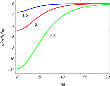
Figure 3: The charge flux along the compact dimension, $a^{D}n_{l}^{(l)}\langle j^{l}\rangle$, as a function of the field mass for different values of the ratio $z/L$ (numbers near the curves). The graphs are plotted for $\tilde{\alpha}=\pi/2$.

From the covariant conservation equation for the current density it follows that the charge flux through the hypersurface element $d^{D-1}x=dz\prod\limits_{i=1,\neq l}^{D-1}dx^{i}$ is given by $\sqrt{|g|}j^{l}d^{D-1}x$. For the expectation value of the total charge flux, per unit coordinate surface along spatial dimensions $(x^{1},\ldots,x^{l-1},x^{l+1},\ldots,x^{D-1})$, integrated over $z$, one gets $\int_{0}^{\infty}dz\,\left(a/z\right)^{D+1}\langle j^{l}\rangle$. From the asymptotic analysis of the current density near the AdS boundary and horizon, given above, we can see that the integral is convergent in the lower limit and linearly diverges in the upper limit. Hence, similar to the Minkowskian case, the total charge flux diverges.

Comparing the fermionic current density in the Minkowski bulk, Eq. (3.11), with the corresponding expression from Ref. [7] for the current density $\langle j^{l}\rangle_{\mathrm{M}}^{\mathrm{(s)}}$ of a charged scalar field, we see that

$$\langle j^{l}\rangle_{\mathrm{M}}=-(N/2)\langle j^{l}\rangle_{\mathrm{M}}^{\mathrm{(s)}},$$ (3.18)

provided the masses, charges and the phases in the periodicity conditions are the same for fermionic and scalar fields. In particular, in supersymmetric models with the same number of fermionic and scalar degrees of freedom, the total current in the Minkowski bulk vanishes. This is not the case for the AdS bulk (for a discussion of boundary conditions on the AdS boundary in supersymmetric models see, for example, Refs. [27, 28] and references therein). Note that for supersymmetric models in AdS background the fields in the same multiplet do not necessarily have the same mass (see, e.g., Refs. [27, 30]). By taking into account the expression of the current density for scalar fields [4], for the total current in the system of a fermionic field and $N/2$ charged scalar fields (equal number of fermionic and scalar degrees of freedom) one gets

$$\langle j^{l}\rangle^{\mathrm{(t)}} = \frac{Nea^{-1-D}L_{l}}{(2\pi)^{(D+1)/2}}\sum_{n_{l}=1}^{\infty}n_{l}\sin(\tilde{\alpha}_{l}n_{l})\sum_{\mathbf{n}_{q-1}}\,\cos(\tilde{\mathbf{\alpha}}_{q-1}\cdot\mathbf{n}_{q-1})$$ (3.19)

$$\times\left[2q_{\nu_{s}-1/2}^{(D+1)/2}(b_{\mathbf{n}_{q}})-q_{ma}^{\left(D+1\right)/2}(b_{\mathbf{n}_{q}})-q_{ma-1}^{\left(D+1\right)/2}(b_{\mathbf{n}_{q}})\right],$$

where $\nu_{s}=\sqrt{D^{2}/4-D(D+1)\xi+m^{2}a^{2}}$ and $\xi$ is the curvature coupling parameter for scalar fields. Near the AdS horizon, the leading contribution from the scalar and fermionic parts in Eq. (3.19) cancel each other and we need to keep the next-to-leading term in the asymptotic (3.13). This leads to the result

$$\langle j^{l}\rangle^{\mathrm{(t)}} \approx \frac{D(D+1)NeL_{l}}{4\pi^{(D+1)/2}a^{D+1}}\Gamma\left(\frac{D-1}{2}\right)\left(\xi-\xi_{D}\right)z^{D-1}$$ (3.20)

$$\times\sum_{n_{l}=1}^{\infty}n_{l}\sin(\tilde{\alpha}_{l}n_{l})\sum_{\mathbf{n}_{q-1}}\,\frac{\cos(\tilde{\mathbf{\alpha}}_{q-1}\cdot\mathbf{n}_{q-1})}{g_{\mathbf{n}_{q}}^{D-1}},$$

in the limit $z\rightarrow\infty$. Here, $\xi_{D}=(D-1)/(4D)$ is the value of the curvature coupling parameter for conformal coupling. The leading term, given by Eq. (3.20), does not depend on the mass. For $ma<1/2$ or $ma\geqslant 1/2$ and $D(D+1)\left(\xi-\xi_{D}\right)<ma$, the fermionic part dominates near the AdS boundary and the total VEV $\langle j^{l}\rangle^{\mathrm{(t)}}$ behaves as in Eq. (3.12). In particular, the latter is the case for minimally coupled scalar fields. For $ma\geqslant 1/2$ and $D(D+1)\left(\xi-\xi_{D}\right)>ma$, the total current density near the AdS boundary is dominated by the scalar contribution and $\langle j^{l}\rangle^{\mathrm{(t)}}\propto z^{D+2\nu_{s}+2}$ for $z\rightarrow 0$.

In Fig. 4, the dependence on the mass of the total charge flux is plotted in the $(p,q)=(3,1)$ model with a fermionic field and $N/2$ scalar fields. The graphs are plotted for $\tilde{\alpha}=\pi/2$ and the numbers near the curves correspond to the values of the ratio $z/L$. The left and right panels are for conformally and minimally coupled scalar fields. In both cases the total current is dominated by the fermionic contribution. In general, the current density is not a monotonic function of the mass.

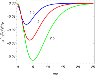
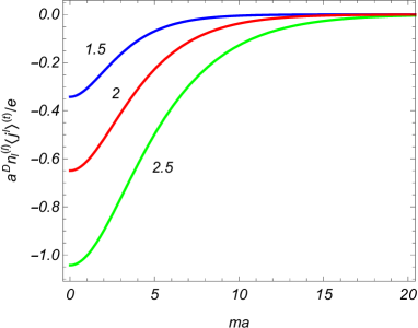
Figure 4: The total charge flux in $(p,q)=(3,1)$ model with a fermionic field and $N/2$ scalar fields as a function of the mass. The left/right panels correspond to conformally/minimally coupled scalar fields. The graphs are plotted for $\tilde{\alpha}=\pi/2$ and the numbers near the curves correspond to the values of the ratio $z/L$.

As seen from Eq. (3.20), compared to the separate scalar and fermionic contributions, the divergence of the total current density on the horizon is weaker and, as a consequence of that, the charge flux integrated over the $z$-coordinate is finite. By using in Eq. (3.19) the integral representation (B.6) for the function $q_{\nu}^{\left(D+1\right)/2}(u)$, after the evaluation of the integral over $z$, the $x$-integral is reduced to $\int_{0}^{\infty}dx\,e^{-x}g(x)$ with $g(x)=\sum_{j=\pm 1/2}I_{ma+j}(x)-2I_{\nu_{s}}(x)$. Though this integral is convergent, the separate integrals with the modified Bessel functions diverge. In order to have the right to take the integrals separately, we can replace the integral by $\int_{0}^{\infty}dx\,e^{-bx}g(x)$, $b>1$. After the evaluation of the separate integrals by using the formula from Ref. [31], the limit $b\rightarrow 1$ is taken easily. In this way, for the integrated charge flux we get

$$\int_{0}^{\infty}dz\,\left(\frac{a}{z}\right)^{D+1}\langle j^{l}\rangle^{\mathrm{(t)}}=\left(ma-\nu_{s}\right)\frac{\Gamma(D/2)eNL_{l}}{2(4\pi)^{D/2}}\sum_{n_{l}=1}^{\infty}n_{l}\sin(\tilde{\alpha}_{l}n_{l})\sum_{\mathbf{n}_{q-1}}\,\frac{\cos(\tilde{\mathbf{\alpha}}_{q-1}\cdot\mathbf{n}_{q-1})}{g_{\mathbf{n}_{q}}^{D}}.$$ (3.21)

It is of interest to note that the mass enters in the factor $\left(ma-\nu_{s}\right)$ only.

4 Fermionic current in C-,P- and T-symmetric odd-dimensional models on AdS bulk

In the discussion above we have evaluated the VEV of the fermionic current density for a field realizing the irreducible representation of the Clifford algebra. It is known that (see, for example, Ref. [32]) in even values of the spatial dimension $D$ (odd-dimensional spacetimes) the mass term $m\bar{\psi}\psi$ in the Lagrangian density breaks $P$-invariance, $C$-invariance for $D=4n$, and $T$-invariance in $D=4n+2$ with $n=0,1,2,\ldots$. $P$-, $C$-, and $T$-invariant models can be constructed combining two fermionic fields in the irreducible representations. In this section we assume that the flat spacetime Dirac matrices are taken in the representation (A.1). For odd-dimensional spacetimes the matrix $\gamma^{(D)}$ can be expressed in terms of the product $\gamma=\gamma^{(0)}\gamma^{(1)}\cdots\gamma^{(D-1)}$ in two inequivalent ways, namely, $\gamma^{(D)}=\gamma_{(s)}^{(D)}=s\gamma$, $s=\pm 1$, for $D=4n$ and $\gamma^{(D)}=\gamma_{(s)}^{(D)}=si\gamma$ for $D=4n+2$. The upper and lower signs correspond to two inequivalent representations of the corresponding Clifford algebra with the gamma matrices $\gamma_{(s)}^{(\mu)}=(\gamma^{(0)},\gamma^{(1)},\cdots\gamma^{(D-1)},\gamma_{(s)}^{(D)})$. The corresponding matrices in AdS spacetime can be taken as $\gamma_{(s)}^{\mu}=(a/z)\gamma_{(s)}^{(\mu)}$.

Consider a system of two $N$-component fermionic fields, $\psi_{(+1)}$ and $\psi_{(-1)}$, with the combined Lagrangian density $\mathcal{L}=\sum_{s=\pm 1}\bar{\psi}_{(s)}(i\gamma_{(s)}^{\mu}\nabla_{\mu}^{(s)}-m)\psi_{(s)}$, $\nabla_{\mu}^{(s)}=\partial_{\mu}+\Gamma_{\mu}^{(s)}$. By suitable transformations of the fields (in general, mixing the separate fields) it can be seen that the Lagrangian density is invariant under the $C$-, $P$- and $T$-transformations (see, e.g., Ref. [32]). By taking into account the relations $\gamma^{(0)}\gamma^{\dagger}\gamma^{(0)}\gamma=-1$ and $\gamma^{(0)}\gamma^{\dagger}\gamma^{(0)}\gamma_{(+1)}^{\mu}\gamma=\gamma_{(-1)}^{\mu}$, the Lagrangian density can also be rewritten as

$$\mathcal{L}=\sum_{s=\pm 1}\bar{\psi}_{(s)}^{\prime}(i\gamma^{\mu}\nabla_{\mu}-sm)\psi_{(s)}^{\prime}.$$ (4.1)

with $\psi_{(+1)}^{\prime}=\psi_{(+1)}$, $\psi_{(-1)}^{\prime}=\gamma\psi_{(-1)}$, and $\gamma^{\mu}=\gamma_{(+1)}^{\mu}$. As seen, the new field $\psi_{(-1)}^{\prime}$ satisfies the same equation as $\psi_{(+1)}$ with the opposite sign for the mass term. Introducing $2N\times 2N$ Dirac matrices $\gamma^{(2N)\mu}=\sigma_{\mathrm{P}3}\otimes\gamma^{\mu}$, with $\sigma_{\mathrm{P}3}=\mathrm{diag}(1,-1)$ being the Pauli matrix, the Lagrangian density is presented in terms of the $2N$-component spinor $\Psi=(\psi_{(+1)}^{\prime},\psi_{(-1)}^{\prime})^{T}$ in the form

$$\mathcal{L}=\bar{\Psi}[i\gamma^{(2N)\mu}(\partial_{\mu}+\Gamma_{\mu}^{(2N)})-m]\Psi,$$ (4.2)

where $\Gamma_{\mu}^{(2N)}=I\otimes\Gamma_{\mu}$.

In the system of two fermionic fields realizing two inequivalent representations of the Clifford algebra, the total current density $J^{\mu}=e\bar{\Psi}\gamma^{(2N)\mu}\Psi$ is given by $J^{\mu}=\sum_{s=\pm 1}j_{(s)}^{\mu}$, where $j_{(s)}^{\mu}=e\bar{\psi}_{(s)}\gamma_{(s)}^{\mu}\psi_{(s)}$ are the current densities for separate fields. As it has been shown in Appendix A, if the phases in the quasiperiodicity conditions along compact dimensions are the same for the fields $\psi_{(+1)}$ and $\psi_{(-1)}$ then the VEVs of the corresponding current densities are the same. In this case, the VEV $\langle J^{l}\rangle$ is obtained from the expressions for $\langle j^{l}\rangle$ given above with an additional coefficient 2. However, the phases $\alpha_{l}$ for the fields $\psi_{(+1)}$ and $\psi_{(-1)}$, in general, can be different.

Among the most interesting physical realizations of fermionic systems in odd-dimensional spacetimes is the graphene. Graphene is an one-atom thick layer of graphite. The low-energy excitations of the corresponding electron subsystem can be described by a pair of two-component spinors, composed of the Bloch states residing on the two triangular sublattices $A$ and $B$ of the graphene honeycomb lattice. For the spatial dimension in the corresponding effective field theory one has $D=2$. For a given value of spin $S=\pm 1$, two spinors are combined in a 4-component spinor $\Psi_{S}=(\psi_{+,AS},\psi_{+,BS},\psi_{-,AS},\psi_{-,BS})^{T}$. The components $\psi_{\pm,AS}$ and $\psi_{\pm,BS}$ correspond to the amplitude of the electron wave function on sublattices $A$ and $B$ and the indices $+$ and $-$ correspond to inequivalent points, $\mathbf{K}_{+}$ and $\mathbf{K}_{-}$ of the Brillouin zone (see Refs. [33, 34]). The values of the parameter $s=+1$ and $s=-1$ in the discussion above, specifying the irreducible representations of the Clifford algebra, correspond to these points. Consequently, we can identify $\psi_{(s)}=(\psi_{s,AS},\psi_{s,BS})^{T}$. For the bulk geometry with vanishing 0th component of the spin connection, $\Gamma_{0}=0$, and for the zero scalar potential of the external electromagnetic field (these conditions are the case in the problem at hand) the combined Lagrangian density, in standard units, is presented as

$$L=\sum_{S=\pm 1}\bar{\Psi}_{S}(i\hbar\gamma^{(4)0}\partial_{t}+i\hbar v_{F}\gamma^{(4)l}D_{l}-\Delta)\Psi_{S}.$$ (4.3)

Here, $v_{F}\approx 7.9\times 10^{7}$ cm/s is the Fermi velocity of the electrons in graphene, $D_{l}=(\mathbf{\nabla}-ie\mathbf{A}/\hbar c)_{l}$, with $l=1,2$, is the spatial part of the gauge extended covariant derivative, and for electrons $e=-|e|$. The energy gap $\Delta$ can be created by a number of mechanisms (see, for instance, Ref. [34] and references therein) and it is related to the Dirac mass $m$ through $\Delta=mv_{F}^{2}$. For the analog of the Compton wavelength corresponding to the energy gap one has $a_{\mathrm{C}}=\hbar v_{F}/\Delta$. The energy scale in the system is determined by the combination $\gamma_{F}=\hbar v_{F}/a_{0}$ ($\approx 2.51$ eV), where $a_{0}\approx 1.42$ Å is the inter-atomic spacing of the graphene lattice. In terms of this combination one has $a_{\mathrm{C}}=a_{0}\gamma_{F}/\Delta$. The Lagrangian densities (4.3) for separate $S$ are the analog of Eq. (4.2) for $D=2$.

For a planar graphene sheet the spatial topology in the corresponding effective field theory is $R^{2}$. In the case of a sheet rolled into a cylinder (cylindrical carbon nanotubes) or torus (toroidal nanotubes) the topology becomes nontrivial: $R^{1}\times S^{1}$ and $S^{1}\times S^{1}$, respectively. In these systems, the magnetic fluxes $\Phi_{l}$ ($l=2$ for cylindrical nanotubes and $l=1,2$ for toroidal ones) we have introduced above, acquire real physical meaning. The carbon nanotubes are characterized by chiral vector $\mathbf{C}_{h}=n_{a}\mathbf{a}+n_{b}\mathbf{b}$, where $n_{a}$, $n_{b}$ are integers and $\mathbf{a}=(\sqrt{3},0)a_{0}$, $\mathbf{b}=(-\sqrt{3},3)a_{0}/2$ are primitive translation vectors of the graphene hexagonal lattice (for general properties of carbon nanotubes, see, for example, Ref. [35]). Note that $\sqrt{3}a_{0}$ is the lattice constant. In the construction of the nanotube the hexagon at the origin is identified with the hexagon at $\mathbf{C}_{h}$. For zigzag and armchair nanotubes one has $n_{b}=0$ and $n_{a}=2n_{b}$, respectively. The other pairs $(n_{a},n_{b})$ correspond to chiral nanotubes. In the case $n_{a}+n_{b}=3q_{c}$, $q_{c}\in Z$, the nanotube will be metallic and for $n_{a}+n_{b}\neq 3q_{c}$ the nanotube will be semiconducting. In the latter case, the corresponding energy gap is inversely proportional to the diameter. In particular, the armchair nanotube is metallic and the $(n_{a},0)$ zigzag nanotube is metallic if and only if $n_{a}$ is an integer multiple of 3. The chirality also determines the periodicity condition along the compact dimension for the fields $\psi_{(s)}$. In the absence of the magnetic flux threading the nanotube, the periodicity conditions have the form $\psi_{(s)}(\mathbf{r}+\mathbf{C}_{h})=e^{-2s\pi ip_{c}/3}\psi_{(s)}(\mathbf{r}+\mathbf{C}_{h})$, where, for a given nanotube, the parameter $p_{c}=-1,0,+1$ is defined by the relation $n_{a}+n_{b}=3q_{c}+p_{c}$ (see, e.g., the discussion in Ref. [33]). Hence, for the phase we have introduced before, one has $\alpha=-2s\pi ip_{c}/3$. For metallic nanotubes one has the periodic boundary condition, $\alpha=0$, and for semiconducting ones $\alpha=\pm 2\pi/3$. As seen, the phases for the spinors corresponding to the points, $\mathbf{K}_{+}$ and $\mathbf{K}_{-}$ of the Brillouin zone have opposite signs. As a consequence, in the absence of the magnetic flux, the total current density in cylindrical nanotubes vanishes.

The problem under consideration is topologically equivalent to the case of cylindrical nanotubes, though the corresponding spatial geometry is curved (for the generation of curvature in graphene sheets and the corresponding effects on the properties of graphene see, for example, Ref. [36, 37]). In Fig. 5 we have plotted this geometry embedded into a 3-dimensional Euclidean space. The magnetic flux threading the compact dimension is shown as well. The proper length of the compact dimension is decreasing with increasing $z$. Note that, related to the graphene physics, a similar spatial geometry has been discussed in [37]. However, the spacetime geometry we consider here is different.

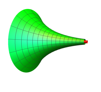
Figure 5: The spatial geometry of a $D=2$ tube embedded in 3-dimensional Euclidean space. The tube of the magnetic flux is shown as well.

Consequently, for a given $S$, the VEVs of the current densities for separate contributions coming from the points $\mathbf{K}_{+}$ and $\mathbf{K}_{-}$ are given by the expressions in previous sections with an additional factor $v_{F}$, and for the nonzero component of the total current one has $\langle J^{1}\rangle=\sum_{s=\pm 1}\langle j_{(s)}^{1}\rangle$, where $j_{(\pm 1)}^{1}$ are the contributions from two valleys. In the problem under consideration separate spins $S$ give the same contributions in the ground state currents. Assuming that the phases $\alpha$ for the contributions from $s=+1$ and $s=-1$ have opposite signs, one finds

$$\langle J^{1}\rangle=-\frac{\sqrt{2}ev_{F}L}{\pi a^{3}}\sum_{n=1}^{\infty}n\cos(\alpha_{(+1)}n)\sin\left(2\pi n\frac{\Phi}{\Phi_{0}}\right)h\left(a/a_{\mathrm{C}},1+\frac{n^{2}L^{2}}{2z^{2}}\right),$$ (4.4)

with the function

$$h\left(\nu,x\right)=2^{\nu}\partial_{x}\left[\frac{1/\sqrt{x-1}}{\left(\sqrt{x+1}+\sqrt{x-1}\right)^{2\nu}}\right].$$ (4.5)

In the absence of the magnetic flux the current density vanishes. In Eq. (4.4), the ratio $a/a_{\mathrm{C}}$ is the analog of the product $ma$ in the discussion of the previous sections. If the curvature of the tube does not change the phases, then $\alpha_{(+1)}=0$ for metallic tubes and $\alpha_{(+1)}=2\pi/3$ for semiconducting ones. Fig. 6 presents the current density in these two cases versus the magnetic flux treading the tube for different values of $a/a_{\mathrm{C}}$ (numbers near the curves). The left/right panels correspond to the metallic/semiconducting tubes. In the numerical evaluation we have taken $z/L=2$.

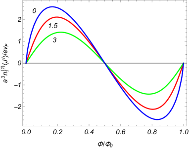
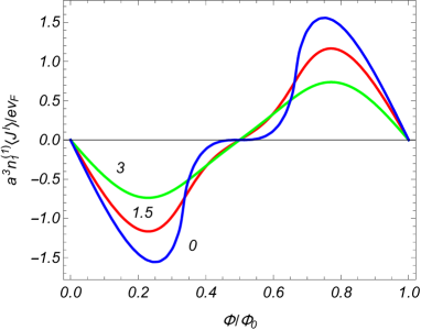
Figure 6: The total charge flux in $D=2$ tubes as a function of the magnetic flux for separate values of $a/a_{\mathrm{C}}$ (numbers near the curves). The left/right panels correspond to metallic/semiconducting tubes. The graphs are plotted for $z/L=2$.

5 Conclusion

In the present paper we have investigated the VEV of the fermionic current density in $(D+1)$-dimensional AdS spacetime with a toroidally compactified subspace. The periodicity conditions for the field operator along compact dimensions contain arbitrary phases $\alpha_{l}$ and, in addition, the presence of a constant abelian gauge field is assumed. By a gauge transformation the problem is reduced to the one in the absence of the gauge field with the shifted phases (2.7) in the quasiperiodicity conditions for the new field. The phase shift for the $l$th compact dimension is formally interpreted in terms of the magnetic flux enclosed by that dimension.

For the evaluation of the vacuum currents we have used the direct summation over the complete set of fermionic modes (2.11) and (2.13). The same result is obtained by using the alternative set of fermionic mode functions (A.6) and (A.7). The VEVs of the charge density and of the components for the current density along uncompact dimensions vanish and the mode sum for the component of the current density along the $l$th compact dimension is presented as Eq. (3.1). A more convenient representation for the renormalized VEV is given by Eq. (3.5). The current density along the $l$th compact dimension is an even periodic function of the phases $\tilde{\alpha}_{i}$, $i\neq l$, and an odd periodic function of the phase $\tilde{\alpha}_{l}$. In particular, this means the periodicity in the magnetic flux with the period equal to the flux quantum. The current density is expressed in terms of the function (B.7). An alternative integral representation is given by Eq. (B.6). Note that the VEV of the current density for a charged scalar field is also expressed through the function (B.7).

In order to clarify the behavior of the current density, various limiting cases of the general result are considered. First of all, we have shown that, in the limit of the infinite curvature radius, the current density for a locally Minkowski bulk is obtained. For a massless field the problem under consideration is conformal to the one in Minkowski spacetime with toral dimensions in the presence of a boundary on which the fermionic field operator obeys the bag boundary condition. However, the boundary-induced contribution in the latter problem vanishes for a massless field and we have obtained a conformal relation with the boundary-free Minkowski case. On the AdS boundary the VEV of the current density vanishes as $z^{D+1+2ma}$, whereas on the AdS horizon it diverges as $z^{D+1}$. Near the horizon the dominant contribution comes from the fluctuations with small wavelengths and the effects induced by the curvature and nonzero mass are small. The influence of the curvature on the component of the current density along the $l$th compact dimension is also small, when the corresponding length $L_{l}$ is much smaller than other length scales in the problem. The leading term in the corresponding asymptotic expansion coincides with the VEV for a massless field in the model with a single compact dimension $x^{l}$. In the opposite limit of large values for the proper length of the $l$th compact dimension, the behavior of the VEV $\langle j^{l}\rangle$ is essentially different depending on the values of the phases in the quasiperiodicity conditions. If all the remaining phases vanish, $\tilde{\alpha}_{i}=0$, $i\neq l$, the current density, as a function of the proper length, behaves as $1/L_{(p)l}^{p+2ma+1}$. Unlike the case of the locally Minkowski bulk, the corresponding decay is power law for both massless and massive fields. If at least one of the phases $\tilde{\alpha}_{i}$, $i\neq l$, is different from zero, the decay of the VEV $\langle j^{l}\rangle$, as a function of $L_{l}$, is exponential.

In the Minkowski bulk, for the system of a fermionic field and $N/2$ charged scalar fields, with the same masses, charges and the same phases in the quasiperiodicity conditions, the total current vanishes as a consequence of the cancellation between the fermionic and scalar contributions. This means that, in the corresponding supersymmetric models, no net current appears. In the AdS bulk the influence of the gravitational field on the VEVs for scalar and fermionic fields, in general, is different and there is no cancellation between the scalar and fermionic counterparts. The corresponding total current density is given by Eq. (3.19). Near the horizon, the leading contributions from the scalar and fermionic parts are canceled, and the first term in the corresponding asymptotic expansion is presented as Eq. (3.20). It does not depend on the mass and vanishes for conformally coupled scalars. As a consequence of the weaker divergence on the horizon, the total charge flux integrated over the $z$-coordinate is finite.

In odd spacetime dimensions the mass term in the Lagrangian density for a fermionic field realizing the irreducible representation of the Clifford algebra, in general, breaks $C$-, $P$-, and $T$-invariances. The models with these symmetries can be constructed combining two fermionic fields realizing two irreducible representations. In section 4 we have considered the current density in this type of models. It has been shown that, if the phases $\alpha_{l}$ are the same for both the representations, their contributions to the total current coincide. However, the phases need not be the same. This type of situation arises in semiconducting cylindrical carbon nanotubes described by an effective Dirac theory in the long-wavelength approximation. In the corresponding Dirac model two irreducible representations correspond to two inequivalent points of the graphene Brillouin zone and, in the absence of the magnetic flux threading the tube, the corresponding phases have opposite signs. We have considered the fermionic current in the corresponding problem on the AdS bulk generated by a magnetic flux.

Appendix A Another class of fermionic modes

In the evaluation of the current density we have used the representation (2.10) for the Dirac matrices and the corresponding fermionic modes (2.11), (2.13). As it has been discussed in Ref. [24], these modes are well adapted for the investigation of the effects induced by the presence of an additional brane, parallel to the AdS boundary, on which the field operator obeys the bag boundary condition. In this appendix we consider another representation of the Dirac matrices that allows for the separation of the equations for the upper and lower components of the fermionic mode functions. In the new representation the flat spacetime gamma matrices are given by

$$\gamma^{(0)}=\left(\begin{array}[]{cc}0&\chi_{0}\\ \chi_{0}^{\dagger}&0\end{array}\right),\;\gamma^{(l)}=\left(\begin{array}[]{cc}0&\chi_{l}\\ -\chi_{l}^{\dagger}&0\end{array}\right),$$ (A.1)

where $l=1,2,\ldots,D-1$, and $\gamma^{(D)}=si\,\mathrm{diag}(1,-1)$ with $s=\pm 1$. In odd-dimensional spacetimes, the values $s=+1$ and $s=-1$ correspond to two irreducible representations of the Clifford algebra. For the $N/2\times N/2$ matrices $\chi_{0}$, $\chi_{l}$ one gets the relations $\chi_{l}\chi_{n}^{\dagger}+\chi_{n}\chi_{l}^{\dagger}=2\delta_{nl}$, $\chi_{l}^{\dagger}\chi_{n}+\chi_{n}^{\dagger}\chi_{l}=2\delta_{nl}$ for $l,n=1,2,\ldots,D-1$, and $\chi_{0}\chi_{l}^{\dagger}=\chi_{l}\chi_{0}^{\dagger}$, $\chi_{0}^{\dagger}\chi_{l}=\chi_{l}^{\dagger}\chi_{0}$, $\chi_{0}^{\dagger}\chi_{0}=1$. As before, the curved spacetime gamma matrices are given by $\gamma^{\mu}=(z/a)\delta_{b}^{\mu}\gamma^{(b)}$. In the special case $D=2$ we have $\chi_{0}=\chi_{1}=1$ and $\gamma^{(0)}=\sigma_{\mathrm{P}1}$, $\gamma^{(1)}=i\sigma_{\mathrm{P}2}$, $\gamma^{(2)}=i\sigma_{\mathrm{P}3}$, where $\sigma_{\mathrm{P}\mu}$ are the Pauli matrices (see, for instance, Ref. [23]).

For the positive-energy modes, decomposing the spinor into the upper and lower components, the separate equations are obtained for them with the solution

$$\psi_{\beta}^{(+)}=z^{\frac{D+1}{2}}e^{i\mathbf{kx}-i\omega t}\left(\begin{array}[]{c}J_{ma+s/2}(\lambda z)\chi^{(\sigma)}\\ \frac{\mathbf{k\chi}^{\dagger}+\omega\chi_{0}^{\dagger}}{\lambda}J_{ma-s/2}(\lambda z)\chi^{(\sigma)}\end{array}\right),$$ (A.2)

where $\chi^{(\sigma)}$, $\sigma=$ $1,\ldots,N/2$, are one-column matrices with $N/2$ rows and $\mathbf{k\chi}^{\dagger}=\sum_{l=1}^{D-1}k_{l}\chi_{l}^{\dagger}$. From the orthonormalization condition for the modes (A.2) one obtains

$$\chi^{(\sigma)\dagger}[\left(\omega+\mathbf{k\chi}\chi_{0}^{\dagger}\right)^{2}+\lambda^{2}]\chi^{(\sigma^{\prime})}=2\lambda^{2}\left|C_{\beta}^{(+)}\right|^{2}\delta_{\sigma\sigma^{\prime}},$$ (A.3)

where $\left|C_{\beta}^{(+)}\right|^{2}$ is given by Eq. (2.15). This shows that we can take

$$\left(\omega+\mathbf{k\chi}\chi_{0}^{\dagger}-i\lambda\right)\chi^{(\sigma)}=\sqrt{2}\lambda C_{\beta}^{(+)}w^{(\sigma)},$$ (A.4)

or inverting

$$\chi^{(\sigma)}=C_{\beta}^{(+)}\frac{\mathbf{k\chi}\chi_{0}^{\dagger}+i\lambda-\omega}{\sqrt{2}i\omega}w^{(\sigma)},$$ (A.5)

where the matrices $w^{(\sigma)}$ are the same as in Eq. (2.11).

As a result, for the positive-energy fermionic modes we get

$$\psi_{\beta}^{(+)}=\frac{C_{\beta}^{(+)}}{\sqrt{2}}z^{\frac{D+1}{2}}e^{i\mathbf{kx}-i\omega t}\left(\begin{array}[]{c}\frac{\mathbf{k\chi}\chi_{0}^{\dagger}+i\lambda-\omega}{\omega}J_{ma+s/2}(\lambda z)w^{(\sigma)}\\ i\chi_{0}^{\dagger}\frac{\mathbf{k\chi}\chi_{0}^{\dagger}+i\lambda+\omega}{\omega}J_{ma-s/2}(\lambda z)w^{(\sigma)}\end{array}\right).$$ (A.6)

In a similar way, for the negative-energy modes one finds the representation

$$\psi_{\beta}^{(-)}=\frac{C_{\beta}^{(-)}}{\sqrt{2}}z^{\frac{D+1}{2}}e^{i\mathbf{kx+}i\omega t}\left(\begin{array}[]{c}i\chi_{0}\frac{\mathbf{k\chi}^{\dagger}\chi_{0}-i\lambda+\omega}{\omega}J_{ma+s/2}(\lambda z)w^{(\sigma)}\\ \frac{\mathbf{k\chi}^{\dagger}\chi_{0}-i\lambda-\omega}{\omega}J_{ma-s/2}(\lambda z)w^{(\sigma)}\end{array}\right).$$ (A.7)

with $C_{\beta}^{(-)}$ defined in Eq. (2.15). As an additional check, it can be seen that the modes (A.6) and (A.7) are orthogonal.

With the modes (A.6) and (A.7), we can evaluate the fermionic current density by using the mode-sum formula (2.9). By taking into account that for a $N/2\times N/2$ matrix $M$ we have $\sum_{\sigma}w^{(\sigma)\dagger}Mw^{(\sigma)}=\mathrm{tr\,}M$, the VEV of the component of the current density along the compact direction $x^{l}$ is presented as

$$\langle j^{l}\rangle=-\frac{eNz^{D+2}}{4(2\pi)^{p}V_{q}a^{D+1}}\sum_{\mathbf{n}_{q}}\int d\mathbf{k}_{(p)}\,\int_{0}^{\infty}d\lambda\frac{k_{l}\lambda}{\omega}\sum_{j=\pm 1}J_{ma+j/2}^{2}(\lambda z).$$ (A.8)

After the integration over the angular part of $\mathbf{k}_{(p)}$ this expression is reduced to Eq. (3.1). As seen, the VEV of the current density does not depend on the parameter $s$ in the definition of the Dirac matrix $\gamma^{(D)}$. In particular, in odd-dimensional spacetimes the current density is the same for two inequivalent irreducible representations of the Clifford algebra. From the derivation of the expression (A.8) it follows that it is also valid for $D=2$ model with the compact dimension of the length $L$. The corresponding expression is obtained putting in Eq. (A.8) $N=2$, $p=0$, $V_{q}=L$, and omitting the integral over $\mathbf{k}_{(p)}$.

Appendix B Evaluation of the mode-sum

Here we evaluate the mode-sum in the definition (3.4) for the function $\mathcal{I}_{\nu}(z)$. By using the integral representation

$$\frac{1}{\omega}=\frac{1}{\sqrt{\pi}}\int_{0}^{\infty}\frac{ds}{s^{1/2}}\,e^{-\omega^{2}s},$$ (B.1)

the integral over $\lambda$ in Eq. (3.4) is expressed in terms of the modified Bessel function $I_{\nu}(z^{2}/2s)$ [31]. After the integration over $k_{(p)}$ one finds

$$\mathcal{I}_{\nu}(z)=\frac{\Gamma(p/2)}{4\sqrt{\pi}}\int_{0}^{\infty}\frac{ds}{s^{(p+3)/2}}e^{-z^{2}/(2s)}I_{\nu+1/2}(z^{2}/2s)\sum_{\mathbf{n}_{q}}k_{l}e^{-k_{(q)}^{2}s}.$$ (B.2)

As the next step we employ the relation

$$\sum_{n_{j}=-\infty}^{+\infty}e^{-sk_{j}^{2}}=\frac{L_{j}}{2\sqrt{\pi s}}\sum_{n_{j}=-\infty}^{+\infty}e^{in_{j}\tilde{\alpha}_{j}}e^{-L_{j}^{2}n_{j}^{2}/(4s)},$$ (B.3)

which is a direct consequence of the Poisson resummation formula. From Eq. (B.3) we can see that

$$\sum_{\mathbf{n}_{q}}k_{l}e^{-k_{(q)}^{2}s}=\frac{-iL_{l}V_{q}}{2^{q+1}\pi^{q/2}s^{q/2+1}}\sum_{\mathbf{n}_{q}}n_{l}e^{i\tilde{\mathbf{\alpha}}\cdot\mathbf{n}_{q}-g_{\mathbf{n}_{q}}^{2}/(4s)},$$ (B.4)

with $\tilde{\mathbf{\alpha}}\cdot\mathbf{n}_{q}=$ $\sum_{i=p+1}^{D-1}n_{i}\tilde{\alpha_{i}}$ and $g_{\mathbf{n}_{q}}$ is defined by Eq. (3.6).

With these relations, the function (3.4) is presented in the form

$$\mathcal{I}_{\nu}(z)=\frac{-iL_{l}V_{q}\Gamma(p/2)}{2^{q-(D-3)/2}\pi^{q/2+1}z^{D+2}}\sum_{\mathbf{n}_{q}}n_{l}e^{i\tilde{\mathbf{\alpha}}\cdot\mathbf{n}_{q}}q_{\nu}^{(D+1)/2}(b_{\mathbf{n}_{q}}),$$ (B.5)

where $b_{\mathbf{n}_{q}}$ is given by Eq. (3.6). Here we have defined the function

$$q_{\nu}^{\left(D+1\right)/2}(u)=\sqrt{\frac{\pi}{2}}\int_{0}^{\infty}dx\,x^{D/2}e^{-ux}I_{\nu+1/2}(x).$$ (B.6)

The integral is expressed in terms of the hypergeometric function and one gets an alternative representation

$$q_{\nu}^{(D+1)/2}(u)=\frac{\sqrt{\pi}\Gamma(\nu+D/2+3/2)}{2^{\nu+1}\Gamma(\nu+3/2)u^{\nu+D/2+3/2}}F\left(\frac{2\nu+D+3}{4},\frac{2\nu+D+5}{4};\nu+\frac{3}{2};\frac{1}{u^{2}}\right).$$ (B.7)

From the definition (B.6) it directly follows that $q_{\nu}^{\left(D+1\right)/2}(u)$ is a monotonically decreasing function of $u>1$ and $\nu>-1/2$. For even number of spatial dimensions, $D=2n$, $n=1,2,\ldots$, the expression (B.7) for the function $q_{\nu}^{\left(D+1\right)/2}(u)$ is further simplified to [4]

$$q_{\nu}^{n+1/2}(u)=(-1)^{n}\sqrt{\frac{\pi}{2}}\partial_{u}^{n}\frac{(u+\sqrt{u^{2}-1})^{-\nu-1/2}}{\sqrt{u^{2}-1}}.$$ (B.8)

In odd dimensional space, $D=2n-1$, the function (B.7) is expressed in terms of the Legendre function of the second kind: $q_{\nu}^{n}(u)=(-1)^{n}\partial_{u}^{n}Q_{\nu}(u)$.

References

- [1] V. M. Mostepanenko and N. N. Trunov, The Casimir Effect and Its Applications (Oxford University Press, Oxford, 1997); K. A. Milton, The Casimir Effect: Physical Manifestation of Zero–Point Energy (World Scientific, Singapore, 2002); M. Bordag, G. L. Klimchitskaya, U. Mohideen, and V. M. Mostepanenko, Advances in the Casimir Effect (Oxford University Press, Oxford, 2009); Casimir Physics, edited by D. Dalvit, P. Milonni, D. Roberts, and F. da Rosa, Lecture Notes in Physics Vol. 834 (Springer-Verlag, Berlin, 2011).
- [2] K. A. Milton, Gravitation Cosmol. 9, 66 (2003); E. Elizalde, J. Phys. A 39, 6299 (2006); B. Green and J. Levin, J. High Energy Phys. 11 (2007) 096; P. Burikham, A. Chatrabhuti, P. Patcharamaneepakorn, and K. Pimsamarn, J. High Energy Phys. 07 (2008) 013; P. Wongjun, Eur. Phys. J. C 75, 6 (2015).
- [3] E. Elizalde, Ten Physical Applications of Spectral Zeta Functions (Springer-Verlag, Berlin, 1995); F. C. Khanna, A. P. C. Malbouisson, J. M. C. Malbouisson, and A. E. Santana, Phys. Rep. 539, 135 (2014).
- [4] E. R. Bezerra de Mello and A.A. Saharian, V.Vardanyan, Phys. Lett. B 741, 155 (2015).
- [5] S. Bellucci, A. A. Saharian, and V. Vardanyan, J. High Energy Phys. 11 (2015) 092.
- [6] S. Bellucci, A. A. Saharian, and V. Vardanyan, Phys. Rev. D 93, 084011 (2016).
- [7] E. R. Bezerra de Mello and A. A. Saharian, Phys. Rev. D 87, 045015 (2013).
- [8] S. Bellucci and A. A. Saharian, Phys. Rev. D 82, 065011 (2010); S. Bellucci, E. R. Bezerra de Mello, and A. A. Saharian, Phys. Rev. D 89, 085002 (2014).
- [9] S. Bellucci, A. A. Saharian, and H. A. Nersisyan, Phys. Rev. D 88, 024028 (2013).
- [10] S. Bellucci and A. A. Saharian, Phys. Rev. D 87, 025005 (2013).
- [11] S. Bellucci, A. A. Saharian, and N. A. Saharyan, Eur. Phys. J. C 75, 378 (2015).
- [12] S. Bellucci, A. A. Saharian, and A. Kh. Grigoryan, Phys. Rev. D 94, 105007 (2016).
- [13] E. R. Bezerra de Mello and A. A. Saharian, Eur. Phys. J. C. 73, 2532 (2013); S. Bellucci, E. R. Bezerra de Mello, A. de Padua, and A. A. Saharian, Eur. Phys. J. C. 74, 2688 (2014); A. Mohammadi, E. R. Bezerra de Mello, and A.A. Saharian, Class. Quantum Grav. 32, 135002 (2015).
- [14] A. Flachi, J. Garriga, O. Pujolàs, and T. Tanaka, J. High Energy Phys. 08 (2003) 053; A. Flachi and O. Pujolàs, Phys. Rev. D 68, 025023 (2003); A.A. Saharian, Phys. Rev. D 73, 044012 (2006); A.A. Saharian, Phys. Rev. D 73, 064019 (2006); A.A. Saharian, Phys. Rev. D 74, 124009 (2006); E. Elizalde, M. Minamitsuji, and W. Naylor, Phys. Rev. D 75, 064032 (2007); R. Linares, H. A. Morales-Técotl, and O. Pedraza, Phys. Rev. D 77, 066012 (2008); M. Frank, N. Saad, and I. Turan, Phys. Rev. D 78, 055014 (2008).
- [15] S. J. Avis, C. J. Isham, and D. Storey, Phys. Rev. D 18, 3565 (1978).
- [16] C. G. Callan, Jr., and F. Wilczek, Nucl. Phys. B 340, 366 (1990).
- [17] J. M. Maldacena, Adv. Theor. Math. Phys. 2, 231 (1998); E. Witten, Adv. Theor. Math. Phys. 2, 253 (1998); S. S. Gubser, I. R. Klebanov, and A. M. Polyakov, Phys. Lett. B 428, 105 (1998).
- [18] L. Randall and R. Sundrum, Phys. Rev. Lett. 83, 3370 (1999); L. Randall and R. Sundrum, Phys. Rev. Lett. 83, 4690 (1999).
- [19] O. Aharony, S. S. Gubser, J. Maldacena, H. Ooguri, and Y. Oz, Phys. Rep. 323, 183 (2000); H. Năstase, Introduction to AdS/CFT correspondence (Cambridge University Press, Cambridge, 2015); M. Ammon and J. Erdmenger, Gauge/Gravity Duality: Foundations and Applications (Cambridge University Press, Cambridge, 2015).
- [20] S. A. Hartnoll, C. P. Herzog, and G. T. Horowitz, Phys. Rev. Lett. 101, 031601 (2008).
- [21] R.-G. Cai, L. Li, L.-F. Li, and R.-Q. Yang, Sci. China-Phys. Mech. Astron. 58(6), 060401 (2015); E. Kiritsis and L. Li, J. High Energy Phys. 01 (2016) 147.
- [22] R. Maartens and K. Koyama, Living Rev. Relativity 13, 5 (2010).
- [23] L. E. Parker and D. J. Toms, Quantum Field Theory in Curved Spacetime: Quantized Fields and Gravity (Cambridge University Press, Cambridge, 2009).
- [24] E. Elizalde, S. D. Odintsov, and A. A. Saharian, Phys. Rev. D 87, 084003 (2013).
- [25] E. R. Bezerra de Mello, E. R. Figueiredo Medeiros, and A. A. Saharian, Class. Quantum Grav. 30, 175001 (2013).
- [26] P. Breitenlohner and D. Z. Freedman, Ann. Phys. 144, 249 (1982); S. Bellucci, Phys. Rev. D 35, 1296 (1987); S. Bellucci, Phys. Rev. D 36, 1127 (1987); M. Henningson and K. Sfetsos, Phys. Lett. B 431, 63 (1998); W. Mueck and K. S. Viswanathan, Phys. Rev. D 58, 106006 (1998).
- [27] A. J. Amsel and D. Marolf, Class. Quant. Grav. 26, 025010 (2009).
- [28] O. Aharony, D. Marolf, and M. Rangamani, J. High Energy Phys. 02 (2011) 041.
- [29] V.E. Ambrus and E. Winstanley, arXiv:1704.00614.
- [30] B. de Wit and I. Herger, arXiv:hep-th/9908005.
- [31] A. P. Prudnikov, Yu. A. Brychkov, and O. I. Marichev, Integrals and series (Gordon and Breach, New York, 1986), Vol.2.
- [32] K. Shimizu, Prog. Theor. Phys. 74, 610 (1985).
- [33] T. Ando, J. Phys. Soc. Japan 74, 777 (2005).
- [34] V. P. Gusynin, S. G. Sharapov, and J. P. Carbotte, Int. J. Mod. Phys. B 21, 4611 (2007); A. H. Castro Neto, F. Guinea, N. M. R. Peres, K. S. Novoselov, and A. K. Geim, Rev. Mod. Phys. 81, 109 (2009).
- [35] R. Saito, G. Dresselhaus, and M. S. Dresselhaus, Physical Properties of Carbon Nanotubes (Imperial College Press, London, 1998); C. Dupas, P. Houdy, and M. Lahmani, Nanoscience: Nanotechnologies and Nanophysics (Springer, Berlin, 2007); S. Bellucci, Phys. Stat. Sol. (c) 2, 34 (2005); S. Bellucci, Nucl. Instr. Meth. Phys. Res. B 234, 57 (2005); J.-C. Charlier, X. Blase, and S. Roche, Rev. Mod. Phys. 79, 677 (2007).
- [36] D. V. Kolesnikov and V. A. Osipov, Phys. Part. Nucl. 40, 502 (2009); M. A. H. Vozmediano, M. I. Katsnelson, and F. Guinea, Phys. Rept. 496, 109 (2010).
- [37] A. Iorio and G. Lambiase, arXiv:1308.0265.