Abstract

An increasing number of use cases require a timely extraction of non-trivial knowledge from semantically annotated data streams, especially on the Web and for the Internet of Things (IoT). Often, this extraction requires expressive reasoning, which is challenging to compute on large streams. We propose Laser, a new reasoner that supports a pragmatic, non-trivial fragment of the logic LARS which extends Answer Set Programming (ASP) for streams. At its core, Laser implements a novel evaluation procedure which annotates formulae to avoid the re-computation of duplicates at multiple time points. This procedure, combined with a judicious implementation of the LARS operators, is responsible for significantly better runtimes than the ones of other state-of-the-art systems like C-SPARQL and CQELS, or an implementation of LARS which runs on the ASP solver Clingo. This enables the application of expressive logic-based reasoning to large streams and opens the door to a wider range of stream reasoning use cases.

1 Introduction

The Web and the emerging Internet of Things (IoT) are highly dynamic environments where streams of data are valuable sources of knowledge for many use cases, like traffic monitoring, crowd control, security, or autonomous vehicle control. In this context, reasoning can be applied to extract implicit knowledge from the stream. For instance, reasoning can be applied to detect anomalies in the flow of information, and provide clear explanations that can guide a prompt understanding of the situation.

Problem. Reasoning on data streams should be done in a timely manner [10, 20]. This task is challenging for several reasons: First, expressive reasoning that supports features for a fine-grained control of temporal information may come with an unfavourable computational complexity. This clashes with the requirement of a reactive system that shall work in a highly dynamic environment. Second, the continuous flow of incoming data calls for incremental evaluation techniques that go beyond repeated querying and re-computation. Third, there is no consensus on the formal semantics for the processing of streams which hinders a meaningful and fair comparison between stream reasoners.

Despite recent substantial progress in the development of stream reasoners, to the best of our knowledge there is still no reasoning system that addresses all three challenges. Some systems can handle large streams but do not support expressive temporal reasoning features [5, 18, 3, 16]. Other approaches focus on the formal semantics but do not provide implementations [13]. Finally, some systems implemented only a particular rule set and cannot be easily generalized [15, 26].

Contribution. We tackle the above challenges with the following contributions.

$\bullet$  We present Laser, a novel stream reasoning system based the recent rule-based framework LARS [8], which extends Answer Set Programming (ASP) for stream reasoning. Programs are sets of rules which are constructed on formulae that contain window operators and temporal operators. Thereby, Laser has a fully declarative semantics amenable for formal comparison.

$\bullet$  To address the trade-off between expressiveness and data throughput, we employ a tractable fragment of LARS that ensures uniqueness of models. Thus, in addition to typical operators and window functions, Laser also supports operators such as $\Box$, which enforces the validity over intervals of time points, and $@$, which is useful to state or retrieve specific time points at which atoms hold.

$\bullet$  We provide a novel evaluation technique which annotates formulae with two time markers. When a grounding of a formula $\varphi$ is derived, it is annotated with an interval $[c,h]$ from a consideration time $c$ to a horizon time $h$, during which $\varphi$ is guaranteed to hold. By efficiently propagating and removing these annotations, we obtain an incremental model update that may avoid many unnecessary re-computations. Also, these annotations enable us to implement a technique similar to the Semi-Naive Evaluation (SNE) of Datalog programs [1] to reduce duplicate derivations.

$\bullet$  We present an empirical comparison of the performance of Laser against the state-of-the-art engines, i.e., C-SPARQL [5] and CQELS [18] using micro-benchmarks and a more complex program. We also compare Laser with an open source implementation of LARS which is based on the ASP solver Clingo to test operators not supported by the other engines.

Our empirical results are encouraging as they show that Laser outperforms the other systems, especially with large windows where our incremental approach is beneficial. This allows the application of expressive logic-based reasoning to large streams and to a wider range of use cases. To the best of our knowledge, no comparable stream reasoning system that combines similar expressiveness with efficient computation exists to date.

2 Theoretical Background: LARS

As formal foundation, we use the logic-based framework LARS [8]. We focus on a pragmatic fragment called Plain LARS first mentioned in [7]. We assume the reader is familiar with basic notions, in particular those of logic programming. Throughout, we distinguish extensional atoms $\mathcal{A}^{\mathcal{E}}$ for input and intensional atoms $\mathcal{A}^{\mathcal{I}}$ for derivations. By $\mathcal{A}=\mathcal{A}^{\mathcal{E}}\cup\mathcal{A}^{\mathcal{I}}$, we denote the set of atoms. Basic arithmetic operations and comparisons are assumed to be given in form of designated extensional predicates, but written with infix notation as usual. We use upper case letters $X,Y,Z$ to denote variables, lower case letters $x,y,\ldots$ are for constants, and $p,a,b,q$ for predicates for atoms.

Definition 1 (Stream). 

A stream ${S=(T,v)}$ consists of a timeline $T$, which is a closed interval in $\mathbb{N}$, and an evaluation function ${v:\mathbb{N}\mapsto 2^{\mathcal{A}}}$. The elements ${t\in T}$ are called time points.

Intuitively, a stream $S$ associates with each time point a set of atoms. We call $S$ a data stream, if it contains only extensional atoms. To cope with the amount of data, one usually considers only recent atoms. Let ${S=(T,v)}$ and ${S^{\prime}=(T^{\prime},v^{\prime})}$ be two streams s.t. ${S^{\prime}\subseteq S}$, i.e., ${T^{\prime}\subseteq T}$ and ${v^{\prime}(t^{\prime})\subseteq v(t^{\prime})}$ for all ${t^{\prime}\in T^{\prime}}$. Then $S^{\prime}$ is called a window of $S$.

Definition 2 (Window function). 

Any (computable) function $w$ that returns, given a stream $S=(T,v)$ and a time point ${t\in\mathbb{N}}$, a window $S^{\prime}$ of $S$, is called a window function.

In this work, we focus on two prominent sliding windows that select recent atoms based on time, respectively counting. A sliding time-based window selects all atoms appearing in the last $n$ time points.

Definition 3 (Sliding Time-based Window). 

Let ${S=(T,v)}$ be a stream, ${t\in T=[t_{1},t_{2}]}$ and let ${n\in\mathbb{N}}$, $n\geq 0$. Then the sliding time-based window function $\tau_{n}$ (for size $n$) is ${\tau_{n}(S,t)=(T^{\prime},v|_{T^{\prime}})}$, where ${T^{\prime}=[t^{\prime},t]}$ and ${t^{\prime}=\max\{t_{1},t-n\}}$.

Similarly, a sliding tuple-based window selects the last $n$ tuples. We define the tuple size $|S|$ of stream $S=(T,v)$ as $|\{(a,t)\mid t\in T,a\in v(t)\}|$.

Definition 4 (Sliding Tuple-based Window). 

Let ${S=(T,v)}$ be a stream, ${t\in T=[t_{1},t_{2}]}$ and let ${n\in\mathbb{N}}$, $n\geq 1$. The sliding tuple-based window function $\#_{n}$ (for size $n$) is

$$\#_{n}(S,t)=\begin{cases}\tau_{t-t^{\prime}}(S,t)&\text{if}~{}|\tau_{t-t^{\prime}}(S,t)|\leq n,\\ S^{\prime}&\text{else,}\end{cases}$$

where $t^{\prime}=\max(\{u\in T\mid|\tau_{t-u}(S,t)|\geq n\}\cup\{t_{1}\})$ and $S^{\prime}=([t^{\prime},t],v^{\prime})$ has tuple size $|S^{\prime}|=n$ such that $v^{\prime}(u)=v(u)$ for all $u\in[t^{\prime}+1,t]$ and $v^{\prime}(t^{\prime})\subseteq v(t^{\prime})$.

Figure 1: A time (resp. tuple) window of size 3 at $t=41$

We refer to these windows simply by time windows, resp. tuple windows. Note that for time windows, we allow size $n=0$, which selects all atoms at the current time point, while the tuple window must select at least one atom, hence $n\geq 1$.

Note that we associate with each time point a set of atoms. Thus, for the tuple-based window, if $[t^{\prime},t]$ is the smallest timeline in which $n$ atoms are found, then in general one might have to delete arbitrary atoms at time point $t^{\prime}$ such that exactly $n$ remain $[t^{\prime},t]$.

Example 1. 

Consider a data stream ${D=(T,v_{D})}$ as shown in Fig. 1, where ${T=[35,42]}$ and $v_{D}=\{36\mapsto\{a(x_{1},y)\},38\mapsto\{a(x_{2},y),b(y,z)\},40\mapsto\{a(x_{3},y)\}\}$. The indicated time window of size 3 has timeline $[38,41]$ and only contains the last three atoms. Thus, the window is also the tuple window of size 3 at 40. Notably, $[38,41]$ is also the temporal extent of the tuple window of size 2, for which there are two options, dropping either $a(x_{2},y)$ or $b(y,z)$ at time 38.

Although Def. 4 introduces nondeterminism, one may assume a deterministic function based on the implementation at hand. Here, we assume data is arriving in a strict order from which a natural deterministic tuple window follows.

Window operators $\boxplus^{w}$. A window function $w$ can be accessed in rules by window operators. That is to say, an expression $\boxplus^{w}\alpha$ has the effect that $\alpha$ is evaluated on the “snapshot” of the data stream delivered by its associated window function $w$. Within the selected snapshot, LARS allows to control the temporal semantics with further modalities, as will be explained below.

2.1 Plain LARS Programs

Plain LARS programs as in [7] extend normal logic programs. We restrict here to positive programs, i.e., without negation.

Syntax. We define the set $\mathcal{A}^{+}$ of extended atoms by the grammar

$$a\mid@_{t}a\mid\boxplus^{w}@_{t}a\mid\boxplus^{w}\Diamond a\mid\boxplus^{w}\Box a\,,$$

where ${a\in\mathcal{A}}$ and $t\in\mathbb{N}$ is a time point. The expressions of form $@_{t}a$ are called $@$-atoms. Furthermore, if $\mathbin{\star}\in\{@_{t},\Diamond,\Box\}$, $\mathbin{\star}a$ is a quantified atom and ${\boxplus^{w}\mathbin{\star}a}$ a window atom. We write $\boxplus^{n}$ instead of $\boxplus^{\tau_{n}}$ for the window operator using a time window function, and $\boxplus^{\#n}$ uses the tuple window of size $n$.

A rule $r$ is of the form $\alpha\leftarrow\beta_{1},\dots,\beta_{n}$, where $\mathit{H}(r)=\alpha$ is the head and $\mathit{B}(r)=\{\beta_{1},\dots,\beta_{n}\}$ is the body of $r$. The head $\alpha$ is of form $a$ or $@_{t}a$, where ${a\in\mathcal{A}^{\mathcal{I}}}$, and each $\beta_{i}$ is an extended atom. A (positive plain) program $P$ is a set of rules. We say an extended atom $\beta$ occurs in a program $P$ if ${\beta\in\{\mathit{H}(r)\}\cup\mathit{B}(r)}$ for some rule ${r\in P}$.

Example 2 (cont’d). 

The rule $r=q(X,Y,Z)\leftarrow\boxplus^{3}\Diamond a(X,Y),\boxplus^{\#3}\Diamond b(Y,Z)$ expresses a query with a join over predicates $a$ and $b$ in the standard snapshot semantics: If for some variable substitutions for $X,Y,Z$, $a(X,Y)$ holds some time during the last 3 time points and $b(Y,Z)$ at some time point in the window of the last 3 tuples, then $q(X,Y,Z)$ is must be inferred.

We identify rules $\alpha\leftarrow\beta_{1},\dots,\beta_{n}$ with implications $\beta_{1}\land\dots\land\beta_{n}\rightarrow\alpha$, thus obtaining by them and their subexpressions the set $\mathcal{F}$ of formulae.

Semantics. We first define the semantics of ground programs, i.e., programs without variables, based on a structure $M=\langle S,W,\mathcal{B}\rangle$, where $S=(T,v)$ is a stream, $W$ a set of window functions, and $\mathcal{B}$ a static set of atoms called background data. Throughout, we use $W=\{\tau_{n},\#_{n}\mid n\in\mathbb{N}\}$. We define when extended atoms $\beta$ (and its subformulae) hold in a structure $M$ at a given time point $t\in T$ as follows. Let $a\in\mathcal{A}$ and $\varphi$ be a quantified atom. Then,

$$\begin{array}[]{l@{\quad\text{iff}\quad}l}M,t\Vdash a&{a\in v(t)}~{}\text{or}~{}{a\in\mathcal{B}},\\ M,t\Vdash\Diamond a&M,t^{\prime}\Vdash a~{}\text{for some}~{}t^{\prime}\!\in T,\\ M,t\Vdash\Box a&M,t^{\prime}\Vdash a~{}\text{for all}~{}t^{\prime}\!\in T,\\ M,t\Vdash@_{t^{\prime}}a&M,t^{\prime}\Vdash a~{}\text{and}~{}t^{\prime}\in T,\\ M,t\Vdash\boxplus^{w}\varphi&M^{\prime},t\Vdash\varphi,~{}\text{where}~{}M^{\prime}=\langle w(S,t),W,\mathcal{B}\rangle.\end{array}$$

For a data stream ${D=(T,v_{D})}$, any stream ${I=(T,v)\supseteq D}$ that coincides with $D$ on $\mathcal{A}^{\mathcal{E}}$ is an interpretation stream for $D$, and a structure ${M=\langle I,W,\mathcal{B}\rangle}$ an interpretation for $D$. Satisfaction by $M$ at ${t\in T}$ is as follows: For a rule $r$ of form $\alpha\leftarrow\beta_{1},\dots,\beta_{n}$, we first define $M,t\models\mathit{B}(r)$ iff $M,t\Vdash\beta_{i}$ for all $i\in\{1,\dots,n\}$. Then, ${M,t\models r}$ iff ${M,t\Vdash\alpha}$ or ${M,t\not\models B(r)}$; $M$ is a model of program $P$ (for $D$) at time $t$, denoted ${M,t\models P}$, if ${M,t\models r}$ for all ${r\in P}$; and $M$ is minimal, if in addition no model ${M^{\prime}=\langle S^{\prime},W,\mathcal{B}\rangle\neq M}$ of $P$ exists s.t. $S^{\prime}=(T,v^{\prime})$ and ${v^{\prime}\subseteq v}$.

Definition 5 (Answer Stream). 

An interpretation stream $I$ is an answer stream of program $P$ for the data stream ${D\subseteq I}$ at time $t$, if ${M=\langle I,W,\mathcal{B}\rangle}$ is a minimal model of the reduct $P^{M,t}=\{r\in P\mid M,t\models\mathit{B}(r)\}$.

Note that using tuple windows over intensional data seems neither useful nor intuitive. For instance, program $P=\{a\leftarrow\boxplus^{\#1}\Diamond b\}$ is inconsistent for a data stream $D$ at time $t$, where the last atom is $b$, occurring at time $t-1$: by deriving $a$ for time $t$, suddenly $a$ would be the last tuple.

Proposition 1. 

Let $P$ be a positive plain LARS program that employs only time windows, and tuple window operators only over extensional atoms. Then, $P$ always has a unique answer stream.

Non-ground programs. We obtain the semantics for non-ground programs in a straightforward way by considering rules with variables as schematic descriptions of respective ground instantiations. Substitutions $\sigma$ are defined as usual.

Example 3 (cont’d). 

Consider the ground program $P$ obtained from rule $r$ of Ex. 2 by replacing variables with constants from the data stream $D$ in Ex. 1:

$$\begin{array}[]{l@{\quad}r@{~~}c@{~~}l}r_{1}\colon&q(x_{1},y,z)~{}~{}&\leftarrow\hfil~{}~{}&\boxplus^{3}\Diamond a(x_{1},y),\boxplus^{\#3}\Diamond b(y,z)\\ r_{2}\colon&q(x_{2},y,z)~{}~{}&\leftarrow\hfil~{}~{}&\boxplus^{3}\Diamond a(x_{2},y),\boxplus^{\#3}\Diamond b(y,z)\\ r_{3}\colon&q(x_{3},y,z)~{}~{}&\leftarrow\hfil~{}~{}&\boxplus^{3}\Diamond a(x_{3},y),\boxplus^{\#3}\Diamond b(y,z)\\ \end{array}$$

At time $t=41$, the time window $\boxplus^{3}$ and the tuple window $\boxplus^{\#3}$ are identical, as indicated in Fig. 1, and contain atoms $a(x_{2},y)$, $b(y,z)$, and $a(x_{3},y)$. Consider rule $r_{1}$. Window atom $\boxplus^{3}\Diamond a(x_{1},y)$ does no hold, since there is not a time point $t$ in the selected window such that $a(x_{1},y)$ holds at $t$. However, the remaining window atoms in $P$ all holds, hence the body of rules $r_{2}$ and $r_{3}$ hold. Thus, a model of $P$ (for $D$ at time 41) must include $q(x_{2},y,z)$ and $q(x_{3},y,z)$. We obtain the answer stream $D\cup(T,\{41\mapsto\{q(x_{2},y,z),q(x_{3},y,z)\}\}$).

Definition 6 (Output). 

Let $I=(T,v)$ be the answer stream of program $P$ (for a data stream $D$) at time $t$. Then, the output (of $P$ for $D$ at $t$) is defined by $v(t)\cap\mathcal{A}^{\mathcal{I}}$, i.e., the intensional atoms that hold at $t$.

Given a data stream $D=(T,v)$, where $T=[t_{1},t_{n}]$, we obtain an output stream $S=(T,v)$ by the output at consecutive outputs, i.e., for each $t^{\prime}\in T$, $v(t^{\prime})$ is the output for $(T^{\prime},v|_{T^{\prime}})$, where $T^{\prime}=[t_{1},t^{\prime}]$. Thus, an output stream is the formal description of the sequence of temporary valid derivations based on a sequence of answer streams over a timeline. Our goal is to compute it efficiently.

Example 4 (cont’d). 

Continuing Example 3, the output of $P$ for $D$ at $41$ is $\{q(x_{2},y,z),q(x_{3},y,z)\}$. The output stream $S=(T,v)$ is given by $v=\{t\mapsto\{q(x_{1},y,z),q(x_{2},y,z)\mid t=38,39\}\cup\{t\mapsto\{q(x_{2},y,z),q(x_{3},y,z)\}\mid t=40,41,42\}$.

3 Incremental Evaluation of LARS Programs

In this section, we describe the efficient output stream computation of Laser. The incremental procedure consists in continuously grounding and then annotating formulae with two time points that indicate when and for how long formulae hold. We thus address two important sources of inefficiency: grounding (including time variables) and model computation.

Our work deliberately focuses on exploiting purely sliding windows. The longer a (potential) step size [8], the less incremental reasoning can be applied. In the extreme case of a tumbling window (i.e., where the window size equals the step size) there is nothing that can be evaluated incrementally. However, as long as the two subsequent windows share some data, the incremental algorithm can be beneficial. We now give the intuition of our approach in an Example.

Example 5 (cont’d). 

Consider again the stream of Fig. 1, and assume that we are at $t=36$, where $a(x_{1},y)$ appears as first atom in the stream. In rule $r=q(X,Y,Z)\leftarrow\boxplus^{3}\Diamond a(X,Y),\boxplus^{\#3}\Diamond b(Y,Z)$, the atom matches the window atom $\alpha=\boxplus^{3}\Diamond a(X,Y)$, and we obtain a substitution $\sigma=\{X\mapsto x_{1},Y\mapsto y\}$ under which $a(X,Y)$ holds at time $36$. However, for $\alpha$, we can use $\sigma$ for the next $3$ time points due to the size of the window and operator $\Diamond$. That is, we start considering $\sigma$ at time $36$ and we have a guarantee that the grounding $\alpha\sigma$ (written postfix) holds until time point $39$, which we call the horizon time. We thus write $\alpha\sigma_{[36,39]}$ for the annotated ground formula, which states that $\boxplus^{3}\Diamond a(x_{1},y)$ holds at all evaluation $t\in[36,39]$, i.e., at $t\in[37,39]$, the neither the grounding nor the truth of $\boxplus^{3}\Diamond a(x_{1},y)$ needs to be re-derived.

Definition 7. 

Let ${\alpha\in\mathcal{F}}$ be a formula, and ${c,h\in\mathbb{N}}$ such that ${c\leq h}$, and $\sigma$ a substitution. Then, ${\alpha\sigma}$ denotes the formula which replaces variables in $\alpha$ by constants due to $\sigma$; $\alpha\sigma_{[c,h]}$ is called an annotated formula, $c$ is called the consideration time and $h$ the horizon time, and the interval $[c,h]$ the annotation.

As illustrated in Ex. 5, the intended meaning of an annotated formula $\alpha\sigma_{[c,h]}$ is that formula $\alpha\sigma$ holds throughout the interval $[c,h]$. Annotations might overlap.

Example 6. 

Consider an atom $a(y)$ streams at time points $5$ and $8$. Then, for the formula $\alpha=\boxplus^{9}\Diamond a(X)$, we get the substitution $\sigma=\{X\mapsto y\}$ and an annotation $a_{1}=[5,14]$ at $t=5$, and then $a_{2}=[8,17]$ at $t=8$. That is to say, $\alpha\sigma=\boxplus^{9}\Diamond a(y)$ holds at all time points $[5,14]$ due to annotation $a_{1}$ and at time points $[8,17]$ due to $a_{2}$, and for each $t\in[8,14]$ it suffices to retrieve one of these annotations to conclude that $\alpha\sigma$ holds at $t$.

We note that the tuple window can be processed dually by additionally introducing a consideration count $c_{\#}$ and a horizon count $h_{\#}$, i.e., an annotated formula $\alpha\sigma_{[c_{\#},h_{\#}]}$ would indicate that $\alpha\sigma$ holds when the number of atoms received so far is between $c_{\#}$ and $h_{\#}$. In essence, the following mechanisms work analogously for time- and tuple-based annotations. We thus limit our presentation to the time-based case for the sake of simplification.

The consideration time allows us to implement a technique similar to semi-naive evaluation (SNE) (see, e.g., VLog [25], RDFox [23], Datalog [1]) which increases efficiency by preventing duplicate derivations. Conceptually, SNE is a method which simply imposes that at least one formula that instantiates the body should be derived during or after the previous execution of the rule, otherwise the rule would surely derive a duplicate derivation. Based on the horizon time, on the other hand, we can quickly determine which formulae should be maintained in the working memory and which ones can be erased because they no longer hold. We delete an annotated formula $\alpha\sigma_{[c,h]}$, as soon as the current time $t$ exceeds $h$. This way of incrementally adding new groundings and immediately removing outdated is more efficient than processing all possible groundings. In particular, it is more efficient to maintain duplicates with temporal overlaps as in Ex. 6 than looking up existing groundings and merging their intervals.

1

2$S_{0},\mathit{I}_{0}\leftarrow\emptyset$; (set of ground formulae)

3 for $t_{i}\in\langle t_{1},\ldots,t_{n}\rangle$ do

4       $S_{i}\leftarrow S_{i-1}\cup\{\,a_{[t_{i},t_{i}]}\mid a\in v_{D}(t_{i})\,\}$;

5       $I_{i}\leftarrow S_{i}\cup\{\,a_{[c,h]}\mid a_{[c,h]}\in I_{i-1}\land t_{i}\leq h\,\}$;

6       while True do

7             $I\leftarrow I_{i}$;

8             for $\alpha\leftarrow\beta_{1},\ldots,\beta_{n}\in P$ do

9                   for $j\in\{1,\ldots,n\}$ do $I_{i}\leftarrow I_{i}\cup\mathit{grd}(\beta_{j},I,t_{1},t_{i})$;

10                   $X\leftarrow\{\alpha\sigma_{[max(c_{1},\ldots,c_{n}),min(h_{1},\ldots,h_{n})]}\mid\beta\sigma_{[c_{1},h_{1}]},\ldots,\beta\sigma_{[c_{n},h_{n}]}\in I_{i}$

11                   $\hskip 24.00005pt\land\,c_{1},\ldots,c_{n}\leq t_{i}\land\bigvee_{j=1}^{n}(c_{j}{=}t_{i})\}$;

12                  

13                  $I_{i}\leftarrow I_{i}\cup X\cup\{\alpha\sigma_{[t_{i},t_{i}]}\mid@_{U}\alpha(\sigma\cup\{U\mapsto t_{i}\})_{[t_{i},h]}\in I_{i}\}$;

14                  

15             end for

16            if $I_{i}=I$  break;

17            

18       end while

19       $v(t_{i})=\{a\in\mathcal{A}^{\mathcal{I}}\mid a_{[c,h]}\in I_{i}\,\land\,c\leq t_{i}\leq h\};$ (can be streamed out if needed)

20 end for

return $S=(T,v)$

Algorithm 1 Evaluation $\mathit{Eval}$. INPUT: Data stream $D{=}(T,v_{D})$, where $T=[t_{1},t_{n}]$; program $P$. OUTPUT: Output stream of $P$ for $D$.

Algorithm 1. We report in Alg. 1 the main reasoning algorithm performed by the system. Sets $I_{1},\ldots,I_{n}$ contain the annotated formulae at times $t_{1},\ldots,t_{n}$; $S_{0},I_{0}$ are convenience sets necessary for the very first iteration. At the beginning of each time point $t_{i}$ we first collect in line 1 all facts from the input stream. Each atom $a\in v(t_{i})$ is annotated with $[t_{i},t_{i}]$, i.e., its validity will expire to hold already at the next time point. In line 1, we expire previous conclusions based on horizon times, i.e., among annotated intensional atoms $a_{[c,h]}$ only those are retained where $t_{i}\leq h$. Note that we do not delete atoms from the data stream.

In lines 1-1, the algorithm performs a fixed-point computation as usual where all rules are executed until nothing else can be derived (line 1). Lines 1-1 describe the physical execution of the rules and the materialization of the new derivations. First, line 1 collects all annotated groundings for extended atoms from the body of the considered rule. We discuss the details of this underlying function $\mathit{grd}$ later (see Alg. 2). In line 1 we then consider any substitution for the body that currently holds $(c_{1},\dots,c_{n}\leq t_{i})$. In order to produce a new derivation, we additionally require at least one formula was not considered in previous time points ($\bigvee_{j=1}^{n}(c_{j}=t_{i})$).

The last condition implements a weak version of SNE, which we call $\mathit{sSNE}$. In fact, it only avoids duplicates between time points and not within the same time point. In order to capture also this last source of duplicates, we would need to add an additional internal counter to track multiple executions of the same rule. We decided not to implement this to limit the space overhead.

Matching substitutions in line 1 then are assigned to the head, where variables which are not used can be dropped as usual. Notice that consideration/horizon time for the ground head atom is given by intersection of all consideration/horizon times of the body atoms, i.e., the guarantee for the derivations is in the longest interval for which the body is guaranteed to hold. If the head is of form $@_{U}\alpha$ and holds now, i.e., at $t_{i}$, we also add an entry for $\alpha$ to $I_{i}$ (line 1). After the fixed-point computation has terminated (line 1), we can either stream the output at $t_{i}$, i.e., $v^{\prime}(t_{i})$ (line 1), or store it for a later output of the answer stream $S$ after processing the entire timeline (line 1).

Algorithm 2. The goal of function $\mathit{grd}$ is to annotate and return all ground formulae which hold now or in the future. Depending on the input formula $\alpha$, the algorithm might perform some recursive calls to retrieve annotated ground subformulae. In particular, this function determines the interval $[c,h]$ from a consideration time $c$ to a horizon time $h$ during which a grounding holds. It is precisely this annotation which allows us to perform an incremental computation and avoid the re-calculation of the entire inference at any time point.

1

2switch $\alpha$ do

3      

4      case $p(\mathbf{x})\colon$ return $\{\alpha\sigma_{[c,h]}\mid\alpha\sigma_{[c,h]}\in I\}$

5      

6      case $\boxplus^{n}\beta\colon$ $S\leftarrow\mathit{grd}(\beta,I,max(0,t_{e}-n),t_{e})$;

7        return $S\cup\{\alpha\sigma_{[c,\min(c+n,h)]}\mid\beta\sigma_{[c,h]}\in S\}$

8      

9      case $\Diamond\beta\colon$ $S\leftarrow\mathit{grd}(\beta,I,t_{b},t_{e})$; return $S\cup\{\alpha\sigma_{[c,\infty]}\mid\beta\sigma_{[c,h]}\in S\}$

10      

11      case $\Box\beta\colon$ $S\leftarrow\mathit{grd}(\beta,I,t_{b},t_{e})$;

12        return $S\cup\{\alpha\sigma_{[t_{e},t_{e}]}\mid\beta\sigma_{[c_{1},h_{1}]},\ldots,\beta\sigma_{[c_{n},h_{n}]}\in S\,\land$

13         $c_{i}\leq c_{i+1},h_{i}\geq c_{i+1}~{}\forall 1\leq i<n\,\land$

14         $c_{1}\leq t_{b}\land t_{e}\leq h_{n}\}\}$

15       case $@_{U}\beta\colon$ $S\leftarrow\mathit{grd}(\beta,I,t_{b},t_{e})$;

16        return $S\cup\{\alpha\sigma_{[c,h]}\mid\alpha\sigma_{[c,h]}\in I\}\,\cup$

17         $\{\alpha\sigma^{\prime}_{[c,\infty]}\mid\beta\sigma_{[c,h]}\in S\land u\in[c,h]\land u\in[t_{b},t_{e}]\land\sigma^{\prime}=\sigma\cup\{U\mapsto u\}\}$

18      

19 end switch

Algorithm 2 Function $\mathit{grd}$. INPUT: Formula $\alpha$, database $I$, beginning time point $t_{b}$, end time point $t_{e}$. OUTPUT: Annotated groundings for $\alpha$.

Function $\mathit{grd}$ works by a case distinction on the form of the input formula $\alpha$, similarly as the entailment relation of the LARS semantics (Section 2). We explain the first three cases directly based on an example.

Example 7 (cont’d). 

As in Ex. 6, assume $\alpha=\boxplus^{9}\Diamond a(X)$ and input atom $a(y)$ at time $5$. Towards annotated groundings of $\alpha$, we first obtain the substitution $\sigma=\{X\mapsto y\}$ which can be guaranteed only for time point $c=5$ for atom $a(X)$, i.e., $a(X)\sigma_{[5,5]}=a(y)_{[5,5]}$. Based on this, we eventually want to compute $\alpha\sigma_{[5,14]}$. This is done in two steps. First, the subformula $\beta=\Diamond a(X)$ is agnostic about the timeline, and its grounding $\beta\sigma$ gets an annotation $[5,\infty]$. The intuition behind setting the horizon time to $\infty$ at this point is that $\Diamond\beta$ will always hold as soon $\beta$ holds once. The restriction to a specific timeline is then carried out when $\beta\sigma_{[5,\infty]}$ is handled in case $\boxplus^{9}\beta$, which limits the horizon to $\min(c+n,\infty)=14$; any horizon time $h$ received for $\beta$ that is smaller than $14$ would remain.

Thus, the conceptual approach of Alg. 2 is to obtain the intervals when a subformula holds and adjust the temporal guarantee either by extending or restricting the annotation. Since the operator $\Box$ evaluates intervals, we have to include the boundaries of the window. That is, if a formula $\boxplus^{n}\Box p({\mathbf{x}})$ must be grounded, we call $\mathit{grd}$ in Alg. 1 for the entire timeline $[t_{1},t_{i}]$, where $t_{i}$ is the current evaluation time. Thus, we get $t_{b}=t_{1},t_{e}=t_{i}$ initially. However, in order for $\Box p({\mathbf{x}})$ to hold under a substitution $\sigma$ within the window of the last $n$ time points, $p({\mathbf{x}})\sigma$ must hold at every time point $[t-n,t]$. Thus, the recursive call for $\boxplus^{n}\beta$ limits the timeline to $[t_{e}-n,t_{e}]$. Then, the case $\Box\beta$ seeks to find a sequence of ordered, overlapping annotations $[c_{1},h_{1}],\dots,[c_{n},h_{n}]$ that subsumes the considered interval $[t_{b},t_{e}]$. In this case, $\Box\beta$ holds at $t_{e}$, but it cannot be guaranteed to hold longer. Thus, when $\alpha\sigma_{[t_{e},t_{e}]}$ is returned to the case for $\boxplus^{n}$, the horizon time will not be extended.

Example 8 (cont’d). 

Consider $\alpha^{\prime}=\boxplus^{2}\Box a(X)$. Assume that in the timeline $[0,7]$ at time points $t=5,6,7$, we received the input $a(y)$, hence $\boxplus^{2}\Box a(y)$ has to hold at $t=7$. When we call (in Alg. 1) $\mathit{grd}(\alpha^{\prime},I,0,7)$, where $I=\{a(y)_{[5,5]},a(y)_{[6,6]},a(y)_{[7,7]}\}$, the case for $\boxplus^{2}\beta$ will call $\mathit{grd}(\Box a(X),I,5,7)$. The sequence of groundings as listed in $I$ subsumes $[5,7]$, i.e., the scope given by $t_{b}=5$ and $t_{e}=7$, and thus the case for $\Box$ returns $\Box a(y)_{[7,7]}$. The annotation remains for $\alpha^{\prime}$, i.e., $\mathit{grd}(\alpha^{\prime},I,0,7)=\{\boxplus^{2}\Box a(y)_{[7,7]}\}$. Note when at time $8$ atom $a(y)$ does not hold, neither does $\boxplus^{2}\Box a(y)$. Hence, in contrast to $\Diamond$, the horizon time is not extended for $\Box$.

With respect to the temporal aspect, the case for $@$ works similarly as the one for $\Diamond$, since both operators amount to existential quantification within the timeline. In addition $\Diamond$, the $@$-operator also includes in the time point substitution $U\mapsto u$ where the subformula $\beta$ holds (line 2). In Line 2, we additionally take from $I$ the explicit derivations for $@$-atoms derived so far.

Proposition 2. 

For every data stream $D$ and program $P$, Alg. 1 terminates.

Proof.

Algorithm 1 contains four loops. The for-loop starting in line 2 ranges over finitely many time points. To see that the inner while-loop (starting at line 5) always terminates, we argue that $I_{i}=I$ eventually holds: Initially, the identity is given in line 6. Next, a finite (and fixed) number of rules is iterated in line 7. For the considered rule head, new groundings $X$ will be derived based on $I_{i}$ and then added to $I_{i}$. For every iteration in the while-loop, each rule is considered only once, and there each body is considered only once in the for-loop in line 8. It remains to argue that $I_{i}$ cannot grow indefinitely, i.e., that in some iteration, no new groundings for body elements are derivable anymore (and thus no new rule firings apply). Leaving aside annotations, the case is as usual, i.e., the condition follows from the fact that the set of input atoms is finite, and thus also the set of possible substitutions; assuming usual safety restriction that there is no recursion through arithmetic expressions or that the set of possible terms (including numbers) is finite. (A practical assumption is, e.g., to limit numbers to those in the timeline.) Thus, possible time references are also bounded, and thus there is a finite number of annotations that can be assigned to any substitution. Consequently, at some point, no further combination of a substitution $\sigma$ and annotation $[c,h]$ can be assigned to a formula, hence the condition in $I_{i}=I$ holds and the while-loop terminates. $\Box$

Theorem 3.1. 

Let $P$ be a positive plain LARS program, $D$ be a data stream with timeline $T=[t_{1},t_{n}]$. Then, $S$ is the output stream of $P$ for $D$ iff $S=\mathit{Eval}(D,P)$.

Sketch.

To show that $\mathit{Eval}(D,P)$ corresponds to the output stream of $P$ for $D$, we first observe that $\mathit{Eval}$ always terminates (Proposition 2). Towards the correctness, we recall that the output stream (for timeline $T=[t_{1},t_{n}]$) is defined as the sequence of consecutive outputs for time points $t_{1},\dots,t_{n}$. This is accounted for by the for-loop from lines 2-16, where line 15 assembles the current output. We obtain the output stream as follows.

In the first iteration we have $t_{i}=t_{1}$. In line 3, $S_{i}=S_{1}$ is initialized with the atoms appearing in the data stream at time $t_{i}$ ($S_{0}$ is empty); $S_{i}$ is copied to $I_{i}$, since all atoms have the annotation $[t_{1},t_{1}]$. The while-loop starting in line 5 then accounts for the fixed point computation for rule derivations, i.e., we will add to $I_{i}$ atoms and @-atoms (more precisely, substitutions with annotations that reflect ground atoms and ground @-atoms) corresponding to heads of rules which hold. Since we consider positive programs, the order in which rules are considered is arbitrary, hence we start a for-loop in line 7 for rule traversal.

In line 8, we collect substitutions for body formulae (and their subformulae) due to the current database $I$ (data and derivations so far) by means of $\mathit{grd}$ (Algorithm 2) which we discuss below. By definition, an element $\beta\sigma_{[c,h]}\in\mathit{grd}(\beta,I,t_{1},t_{i})$ means that formula $\beta$ (which may be ground or non-ground), grounded by substitution $\sigma$, is guaranteed to hold from time $c$ to time $h$ due to the current database $I$, given a timeline from $t_{1}$ to $t_{i}$.

Based on the derived evidence for body elements, we check in line 9 whether the considered rule $\alpha\leftarrow\beta_{1},\dots,\beta_{n}$ fires, i.e., whether there is a substitution $\sigma$ for $\beta_{1},\dots,\beta_{n}$ with annotations $[c_{1},h_{1}],\dots,[c_{n},h_{n}]$, respectively, that can already be considered ($c_{1},\dots,c_{n}\leq t_{i}$). In this case, the head $\alpha$ can be derived; more precisely, the substitution carries over for the rule head with an annotation obtained as intersection of the body annotations, i.e., the latest consideration time and the earliest horizon time. This is largest interval for which the body is guaranteed to hold. To additional condition $\bigvee_{j=1}^{n}(c_{j}=t_{i})$ ensures that at least one of the consideration times $c_{1},\dots,c_{n}$ matches the current time point, i.e., this is only an optimization step to avoid reconsideration of existing derivations at later time points. Accordingly, annotated formulae are stored in $X$.

Next, line 11, these collected inferences are added to $I_{i}$ along with derivations for @-atoms which start to hold now. Note that the database entry $@_{t_{i}}\alpha_{[t_{i},h]}$ means that from time point $t_{i}$ to time point $h$, $\alpha$ holds for time point $t_{i}$, i.e., the mapping $t_{i}\mapsto\alpha$ is guaranteed to hold within $[t_{i},h]$. Formally, ${M,t^{\prime}\Vdash@_{t_{i}}\alpha}$ (in the according structure $M$), where ${t^{\prime}\in[t_{i},h]}$. However, at any time point ${t^{\prime}\in[t_{i}+1,h]}$ we do not obtain a guarantee for $\alpha$ to hold at $t^{\prime}$ (from this entry); i.e., ${M,t^{\prime}\Vdash\alpha}$ for ${t^{\prime}\in[t_{i}+1,h]}$ is not implied. We observe that $@_{t_{i}}\alpha_{[t_{i},h]}$ only implies ${M,t_{i}\Vdash\alpha}$; thus $\alpha\sigma$ is annotated with $[t_{i},t_{i}]$. This concludes the while loop and we end up with annotated formulae $\alpha\sigma_{[c,h]}$ in $I_{i}$ for currently derivable information based on the fixed point computation. Finally, we get by all currently derivable atoms the output $v(t_{i})$ at $t_{i}$, i.e., annotated atoms of form $a_{[c,h]}$ in $I_{i}$, where $a$ is intensional and the current time $t_{i}$ is within $[c,h]$.

For the remaining iterations of the outer for-loop ($t_{i}=t_{2},\dots,t_{n}$), observe that Line 3 simply expands the history of the input stream, and line 4 keeps only those derivations which have not yet expired, i.e., conclusions from previous iterations that do not need to be recomputed.

It remains to show that $\mathit{grd}$ computes the correct substitutions and formulae due to the LARS semantics. Let $\alpha$ be a formula, $I$ be the current database and the timeline be $[t_{b},t_{e}]$ (which is always $[t_{1},t_{i}]$). We want to obtain annotated substitutions for $\alpha$ and its subformulae that reflect when an according ground formula is guaranteed to hold. We do so by a case distinction:

For the case of a predicate $p({\mathbf{x}})$, we simply return the elements of the database obtained so far. In case of a window atom $\boxplus^{n}\beta$, we first retrieve recursively the groundings in a timeline narrowed down as stated by the window, i.e., for the interval $[\max(0,t_{e}-n),t_{e}]$. The $\max$ serves to prevent the extreme case where the window would reach back beyond the end of the stream. Substitutions $\sigma$ returned for $\beta$ are applicable for the window formula, which narrows down the temporal scope of the annotation to $[c,\min(c+n,h)]$, i.e., the consideration time remains and the horizon time is either carried over (if it is natural number) or determined at this point due to the window length (if infinite; see cases below).

For case $\Diamond\beta$, we likewise determine the groundings for $\beta$ in the entire considered (global) interval $[t_{b},t_{e}]$. As such, for any grounding $\beta\sigma_{[c,h]}$ retrievable for $\beta$, $\alpha=\Diamond\beta$ would hold forever, i.e., never expire. Thus, we assign $[c,\infty]$, and only the window operator as discussed above will then limit the horizon time due to its length. (Note that a formula of form $\Diamond\beta$ occurs only in the scope of a window operator.)

The case $\Box\beta$ is dual, i.e., a grounding $\beta\sigma$ has to hold at all time points in a considered interval, and no guarantee is obtained for the next time point. This is reflected in lines 7-9 in Algorithm 2: We look for a substitution $\sigma$ for $\beta$ with consecutive ($c_{i}\leq c_{i+1}$) and overlapping ($h_{i}\geq c_{i+1}$) annotations $[c_{1},h_{1}],\dots,[c_{n},h_{n}]$ such that the considered interval $[t_{b},t_{e}]$ is included in their union. Then, we infer that ${\alpha=\Box\beta}$ holds now (${t_{e}=t_{i}}$ of Algorithm 1), but no further guarantee is available, hence the annotation $[t_{e},t_{e}]$.

For case $@_{U}\beta$ we again first retrieve groundings $\beta\sigma_{[c,h]}$ for subformula $\beta$. Then, for all time points $u\in[c,h]$, due to the definition of the @-operator, $@_{u}\alpha$ holds for every $u$ is contained in the considered timeline $[t_{b},t_{e}]$. That is, we get for any such $u$ a new substitution $\sigma^{\prime}$ by adding to $\sigma$ the binding $U\mapsto u$. Note that $@$ is, like $\Diamond$, an existential quantification over the timeline, which additionally stores the time point. Thus, similarly as in the case for $\Diamond\beta$, $@_{U}\beta\sigma^{\prime}$ gets the annotation $[c,\infty]$ and the outer window operator will limit the scope of the horizon based on its length.

This concludes the proof sketch. $\Box$

Tuple-based windows. As noted earlier, our annotation-based approach based on consideration time $c$ and horizon time $h$ works analogously from the tuple-based window by additionally working with a consideration count $c_{\#}$ and a horizon count $h_{\#}$ for every ground formula. Each formula can then hold and expire in only one of these dimensions, or both of them at the same time.

Example 9. 

Consider again rule $r$ from Ex. 5. When $b(y,z)$ streams in at time $38$ as third atom, we obtain an annotated ground formula $\boxplus^{\#3}\Diamond b(y,z)_{[3\#,5\#]}$. That is, when the fourth and fifth atoms stream in, regardless at which time points, $\boxplus^{\#3}\Diamond b(y,z)$ is still guaranteed to hold.

Adding negation. Notably, our approach can be extended for handling negation as well. In plain LARS as defined in [7], extended atoms $\beta$ from rule bodies may occur under negation. We can, however, instead assume negation to occur directly in front of atoms: Due to the FLP-semantics [12] of LARS [8], where “$\operatorname{not}$” can be identified with $\neg$, we get the following equivalences for both $w\in\{\tau_{n},\#_{n}\}$: ${\neg\boxplus^{w}\Diamond a({\mathbf{x}})}\equiv{\boxplus^{w}\Box\neg a({\mathbf{x}})}$ and ${\neg\boxplus^{w}\Box a({\mathbf{x}})}\equiv{\boxplus^{w}\Diamond\neg a({\mathbf{x}})}$. The case is more subtle for $@$, since $@_{t}\neg a({\mathbf{x}})$ implies that $a({\mathbf{x}})$ is false. However, due to the definition of $@$, $\neg@_{t}a({\mathbf{x}})$ can also hold if $t$ is not contained in the considered timeline. Thus, the equivalence ${\neg\boxplus^{w}@_{t}a({\mathbf{x}})}\equiv{\boxplus^{w}@_{t}\neg a({\mathbf{x}})}$ (necessarily) holds only if the timeline contains $t$. This assumption is safe when we assume that the timeline always covers all considered time points.

Our approach extends naturally to a variant of plain LARS where negation appears only in front of atoms: In addition to the base case $p({\mathbf{x}})$ in Line 2 in Alg. 2 we must add a case for a negative literal $\ell=\neg p({\mathbf{x}})$. Using standard conventions, we then have to consider all possible substitutions $\sigma$ for variables in ${\mathbf{x}}$ that occur positively in the same rule $r$, such that $p({\mathbf{x}})\sigma$ does not hold.

We obtain a fragment that is significantly more expressive, but results in having multiple answer streams in general: note that plain LARS essentially subsumes normal logic programs, and the program $a\leftarrow\operatorname{not}b;~{}b\leftarrow\operatorname{not}a$ has two answer sets $\{a\}$ and $\{b\}$. Analogously, we get multiple answer streams by allowing such loops through negation. To retain both unique model semantics and tractability, we propose restricting to stratified negation, i.e., allowing negation but no loops through negation. Then, we can add to Alg. 1 an additional for-loop around lines 1-1 to compute the answer stream stratum by stratum bottom up as usual. In fact, our implementation makes use of this extension.

4 Evaluation

We evaluate the performance of Laser on two dimensions: First, we measure the impact of our incremental procedures on several operators by micro-benchmarking the system on special single-rule programs. Second, we compare the performance against the state of the art on more realistic programs.

Streams. Unfortunately, we could not use some well-known stream reasoning benchmarks (e.g., SRBench [27], CSRBench [11] LSBench [19], and CityBench [2]) because (i) we need to manually change the window sizes and the speed of stream in order to benchmark our incremental approach, but this is not often supported in these benchmarks; (ii) in order to be effective, a micro-benchmark needs to introduce as little overhead as possible; (iii) we needed to make sure that all reasoners return the same results for a fair comparison, and this was easier with a custom data generator that we wrote for this purpose.

State-of-the-art. In line with current literature, we selected C-SPARQL [5], and CQELS [18] as our main competitors. For LARS operators that are not supported by these engines, we compare Laser with Ticker [9], another recent engine for (non-stratified) plain LARS programs. Ticker comes with two reasoning modes, a fully incremental one, and another one that uses an ASP encoding which is then evaluated by the ASP solver Clingo [14]. The incremental reasoning mode was not available at the time of this evaluation. Thus, our evaluation against Ticker concerns only the reasoning mode which is based on Clingo.

Data generation. Unfortunately, each engine has its own routines for reading the input. As a result, we were compelled to develop custom data generators to guarantee fairness. A key problem is that CQELS processes every new data item immediately after the arrival in contrast to Laser and C-SPARQL that process them in batches. Hence, to control the number of triples that stream into CQELS, and make sure that all engines receive equal number of triples at every time point, we configured each data generator to issue a triple at calculated intervals. For this same reason, we report the evaluation results as the average runtime per input triple and not runtime per time point.

Experimental platform. The experiments were performed on a machine with 32-core Intel(R) Xeon(R) 2.60GHz and 256G of memory. We used Java 1.8 for C-SPARQL and CQELS and PyPy 5.8 for Laser. We set the initial Java heap size to 20G and increase the maximum heap size to 80G to minimize potential negative effects of JVM garbage collection. For Ticker we used Clingo 5.1.0.

Window-Diamond. The standard snapshot semantics employed in C-SPARQL and CQELS selects recent data and then abstracts away the timestamps. In LARS, this amounts to using $\Diamond$ to existentially quantify within a window. Here, we evaluate how efficiently each engine can evaluate this case.

We use the rule $q(A,B)\leftarrow\boxplus^{n}\Diamond p(A,B)$, where a predicate of form $r(A,B)$ corresponds to a triple $\langle A,r,B\rangle$. The window size and the stream rate (i.e. the number of atoms streaming in the system at every time point) are the experiment parameters. We create a number of artificial streams which produces a series of unique atoms with predicate $p$ at different rates; we vary window sizes from 1sec to 80secs and the stream rate from 200 to 800 triples per second (t/s).

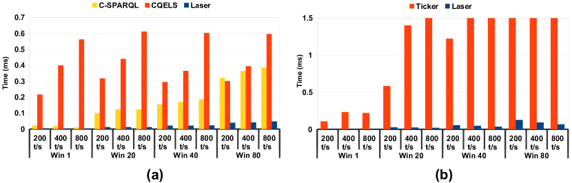
Figure 2: (a) Avg runtime of $\Diamond$ (b) and of $\Box$ on multiple window sizes and stream rates.

Fig. 2(a) reports the average runtime per input triple for each engine. The figure shows that Laser is faster than the other engines. Furthermore, we observe that average runtime of Laser grows significantly slower with the window size as well as with the stream rate. Here, incremental reasoning clearly is beneficial.

Window-Box. The Box operator is not available in C-SPARQL and CQELS. The semantics of $\Box$ (as well as $@$) may be encoded using explicit timestamps in additional triples but the languages themselves do not directly support it. Therefore, we evaluate the performance of Laser against Ticker. Similar to the experiments with $\boxplus\Diamond$, we employ the rule $q(A,B)\leftarrow\boxplus^{n}\Box p(A,B)$. The experimental settings are similar to the previous experiment and results are reported in Fig. 2(b), showing that Laser was orders of magnitude faster than Ticker. Notice that with $\Box$ we cannot extend the horizon time, therefore the incremental evaluation cannot be exploited. Thus, the performance gain stems from maintaining existing substitutions instead of full recomputations.

Data joins. We now focus on a rule which requires a data join. The computation evaluates the rule $q(A,C)\leftarrow\boxplus^{n}\Diamond p(A,B),\boxplus^{n}\Diamond p(B,C)$ with different window sizes/stream rates. This program adds the crucial operation of performing a join. From the results reported in Fig. 3(a), we observe the following:

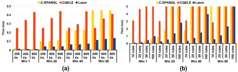
Figure 3: (a) Avg. runtimes when the rule requires a data join (b) Avg. runtimes with multiple rules.

(i) Laser is significantly faster that CQELS and C-SPARQL with all configurations of window and stream sizes. (ii) The difference becomes bigger for larger window sizes for which the benefit of incremental evaluation increases.

We profiled the execution of Laser with the larger windows and stream sizes and discovered that only about half of the time is spent on the join while half is needed to return the results. We also performed an experiment where we deactivated sSNE and did a normal join instead. We observed that sSNE is slightly slower than the normal join with small window sizes, but as the size of windows and stream rate increase, sSNE is significantly faster. In the best case, the activation of sSNE produced a runtime which was 10 times lower.

Evaluating multiple rules. We now evaluate the performance of Laser in a situation where the program contains multiple rules. In C-SPARQL or CQELS, this translates to a scenario where there are multiple standing queries. To do so, we run a series of experiments where we changed the number of rules and the window sizes (stream rate was constant at 200 t/s). To that end, we utilize the same rule that we used in the data join benchmark with the same data generator. Fig. 3(b) presents the average runtime (per triple). We see that also in this case Laser outperforms both C-SPARQL and CQELS, except in the very last case where all systems did not finish on time.

Cooling use case. So far we have evaluated the performance using analytic benchmarks. Now, we measure the performance of Laser with a program that deals with a cooling system. The program of Fig. 4 determines based on a water temperature stream whether the system is working under normal conditions, or it is too hot and produces steam, or is too cold and the water is freezing.

The system also reports temperature readings that are either too high or too low. Note that both $@$ (especially in the rule head) and $\Box$ go beyond standard stream reasoning features. It is not possible to directly translate this program into C-SPARQL or CQELS queries, so we can only compare the performance of Laser with Ticker. In this case, the data generator produces a sequence of random temperature readings. Like before, we gradually increased the window size and stream rate. The results, shown in Fig. 5, indicate that Laser is considerably faster than Ticker and can maintain a good response time ($\leq 100\mu$sec) even when the readings come with high frequency (800 t/s).

$$r_{1}:\;@_{T}\;steam(V)\leftarrow\;\!\boxplus^{n}@_{T}\;\!temp(V),~{}{V\geq 100} r_{6}:\;normal\leftarrow\boxplus^{n}\Box isLiquid$$

$$r_{2}:\;@_{T}\;liquid(V)\leftarrow\;\!\boxplus^{n}@_{T}\;\!temp(V),~{}{V\geq 1},~{}{V<100} r_{7}:\;freeze\leftarrow\operatorname{not}alarm\;\!,\operatorname{not}normal$$

$$r_{3}:\;@_{T}\;\!isSteam\leftarrow\boxplus^{n}\;\!@_{T}\;\!steam(V) r_{8}:\;veryHot(T)\leftarrow\boxplus^{n}\;\!@_{T}\;\!steam(V),{V\geq 150}$$

$$r_{4}:\;@_{T}\;\!isLiquid\leftarrow\boxplus^{n}\;\!@_{T}\;\!liquid(V) r_{9}:\;veryCold(T)\leftarrow\boxplus^{n}\;\!@_{T}\;\!liquid(V),{V=1}$$

$$r_{5}:\;alarm\leftarrow\boxplus^{n}\Box\;\!isSteam$$

Figure 4: Program for a cooling system monitoring.

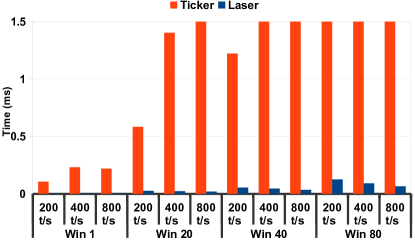
Figure 5: Average execution time per atom of Lars program in Fig 4.

5 Related Work and Conclusion

Related Work. The vision of stream reasoning was proposed by Della Valle et al. in [10]. Since then, numerous publications have studied different aspects of stream reasoning such as: extending SPARQL for stream querying [4, 18], building stream reasoners [4, 18, 21], scalable stream reasoning [15], and ASP models for stream reasoning [13]. However, due to lack of standardized formalism for RDF stream processing, each of these engines provide a different set of features, and results are hard to compare. A survey of these techniques is available at [20]. Our work differs in the sense that it is based on LARS [8], one of the first formal semantics for stream reasoning with window operators.

An area closely related to stream processing is incremental reasoning, which has been the subject of a large volume of research [22, 26]. In this context, [6] describes a technique to add expiration time to RDF triples to drop them when the are no longer valid. Nonetheless, this approach does not support expressive operations such as $\Box$ and $@$ that our engine supports. In a similar way, [17] proposes another incremental algorithm for processing streams which again boils down to efficiently identifying expired information. We showed that our approach outperforms their work. Next, [7] proposes a technique to incrementally update an answer stream of a so-called s-stratified plain LARS program by extending truth maintenance techniques. While [7] focuses on multiple models, we aim at highly efficient reasoning for use cases that guarantee single models. Similarly, the incremental reasoning mode of Ticker [9] focuses on model maintenance but not on high performance. Stream reasoning based on ASP was also explored in a probabilistic context [24] which however did not employ windows.

Conclusion. We presented Laser, a new stream reasoner that is built on the rule-based framework LARS. Laser distinguishes itself by supporting expressive reasoning without giving up efficient computation. Our implementation, freely available, has competitive performance with the current state-of-the-art. This indicates that expressive reasoning is possible also on highly dynamic streams of data. Future work can be done on several fronts: Practically, our techniques extend naturally to further windows operators such as tumbling windows or tuple-based windows with pre-filtering. From a theoretical perspective, the question arises which variations or more involved syntactic fragments of LARS may be considered that are compatible with the presented annotation-based incremental evaluation. Moreover, our support of stratified negation is prototypical and can be made more efficient. More generally, investigations on the system-related research question of reducing the runtimes even further are important to tackle the increasing number and volumes of streams that are emerging from the Web.

References

- [1] Serge Abiteboul, Richard Hull, and Victor Vianu. Foundations of databases, volume 8. Addison-Wesley Reading, 1995.
- [2] Muhammad Intizar Ali, Feng Gao, and Alessandra Mileo. Citybench: A Configurable Benchmark to Evaluate RSP Engines Using Smart City Datasets. In Proceedings of ISWC, pages 374–389, 2015.
- [3] Darko Anicic, Paul Fodor, Sebastian Rudolph, and Nenad Stojanovic. EP-SPARQL: a Unified Language for Event Processing and Stream Reasoning. In Proceedings of WWW, pages 635–644, 2011.
- [4] Davide Francesco Barbieri, Daniele Braga, Stefano Ceri, Emanuele Della Valle, and Michael Grossniklaus. C-SPARQL: SPARQL for Continuous Querying. In Proceedings of WWW, pages 1061–1062. ACM, 2009.
- [5] Davide Francesco Barbieri, Daniele Braga, Stefano Ceri, Emanuele Della Valle, and Michael Grossniklaus. C-SPARQL: a Continuous Query Language for RDF Data Streams. Int. J. Semantic Computing, 4(1):3–25, 2010.
- [6] Davide Francesco Barbieri, Daniele Braga, Stefano Ceri, Emanuele Della Valle, and Michael Grossniklaus. Incremental Reasoning on Streams and Rich Background Knowledge. In Proceedings of ESWC, pages 1–15, 2010.
- [7] Harald Beck, Minh Dao-Tran, and Thomas Eiter. Answer Update for Rule-Based Stream Reasoning. In Proceedings of IJCAI, pages 2741–2747, 2015.
- [8] Harald Beck, Minh Dao-Tran, Thomas Eiter, and Michael Fink. LARS: A Logic-based Framework for Analyzing Reasoning over Streams. In Proceedings of AAAI, pages 1431–1438, 2015.
- [9] Harald Beck, Thomas Eiter, and Christian Folie. Ticker: A System for Incremental ASP-based Stream Reasoning. TPLP (to appear), 2017.
- [10] Emanuele Della Valle, Stefano Ceri, Frank Van Harmelen, and Dieter Fensel. It’s a streaming world! reasoning upon rapidly changing information. IEEE Intelligent Systems, 24(6):83–89, 2009.
- [11] Daniele Dell’Aglio, Jean-Paul Calbimonte, Marco Balduini, Oscar Corcho, and Emanuele Della Valle. On Correctness in RDF Stream Processor Benchmarking. In Proceedings of ISWC, pages 326–342, 2013.
- [12] Wolfgang Faber, Nicola Leone, and Gerald Pfeifer. Recursive Aggregates in Disjunctive Logic Programs: Semantics and Complexity. In JELIA, 2004.
- [13] Martin Gebser, Torsten Grote, Roland Kaminski, Philipp Obermeier, Orkunt Sabuncu, and Torsten Schaub. Answer set programming for stream reasoning. arXiv preprint arXiv:1301.1392, 2013.
- [14] Martin Gebser, Roland Kaminski, Benjamin Kaufmann, and Torsten Schaub. Clingo = ASP + control: Preliminary report. CoRR, abs/1405.3694, 2014.
- [15] Jesper Hoeksema and Spyros Kotoulas. High-performance Distributed Stream Reasoning Using S4. In Ordring Workshop at ISWC, 2011.
- [16] Srdjan Komazec, Davide Cerri, and Dieter Fensel. Sparkwave: Continuous Schema-enhanced Pattern Matching over RDF Data Streams. In DEBS, pages 58–68, 2012.
- [17] Danh Le-Phuoc. Operator-aware Approach for Boosting Performance in RDF Stream Processing. Web Semantics: Science, Services and Agents on the World Wide Web, 42:38–54, 2017.
- [18] Danh Le-Phuoc, Minh Dao-Tran, Josiane Xavier Parreira, and Manfred Hauswirth. A Native and Adaptive Approach for Unified Processing of Linked Streams and Linked Data. In Proceedings of ISWC, pages 370–388, 2011.
- [19] Danh Le-Phuoc, Minh Dao-Tran, Minh-Duc Pham, Peter Boncz, Thomas Eiter, and Michael Fink. Linked Stream Data Processing Engines: Facts and Figures. Proceedings of ISWC, pages 300–312, 2012.
- [20] Alessandro Margara, Jacopo Urbani, Frank Van Harmelen, and Henri Bal. Streaming the web: Reasoning over dynamic data. Web Semantics: Science, Services and Agents on the World Wide Web, 25:24–44, 2014.
- [21] Alessandra Mileo, Ahmed Abdelrahman, Sean Policarpio, and Manfred Hauswirth. StreamRule: a Nonmonotonic Stream Reasoning System for the Semantic Web. In International Conference on Web Reasoning and Rule Systems, pages 247–252, 2013.
- [22] Boris Motik, Yavor Nenov, Robert Piro, and Ian Horrocks. Incremental Update of Datalog Materialisation: The Backward/Forward Algorithm. In Proceedings of AAAI, pages 1560–1568, 2015.
- [23] Yavor Nenov, Robert Piro, Boris Motik, Ian Horrocks, Zhe Wu, and Jay Banerjee. RDFox: A Highly-scalable RDF Store. In Proceedings of ISWC, pages 3–20, 2015.
- [24] Matthias Nickles and Alessandra Mileo. A Hybrid Approach to Inference in Probabilistic Non-Monotonic Logic Programming. In Proceedings of the 2nd International Workshop on Probabilistic Logic, pages 57–68, 2015.
- [25] Jacopo Urbani, Ceriel Jacobs, and Markus Krötzsch. Column-Oriented Datalog Materialization for Large Knowledge Graphs. In Proceedings of AAAI, pages 258–264, 2016.
- [26] Jacopo Urbani, Alessandro Margara, Ceriel Jacobs, Frank Van Harmelen, and Henri Bal. Dynamite: Parallel Materialization of Dynamic RDF Data. In Proceedings of ISWC, pages 657–672, 2013.
- [27] Ying Zhang, Pham Duc, Oscar Corcho, and Jean-Paul Calbimonte. SRBench: a Streaming RDF/SPARQL Benchmark. Proceedings of ISWC, pages 641–657, 2012.