Swimming in spacetime: the view from a Fermi observer

Abstract

An extended test body moving in a curved spacetime does not typically follow a geodesic, because of forces that arise from couplings between its multipole moments and the ambient curvature. An illustration of this fact was provided by Wisdom, who showed that the motion of a quasi-rigid body undergoing cyclic changes of shape in a curved spacetime deviates, in general, from a geodesic. Wisdom’s analysis, however, was recently challenged on the grounds that the body’s motion should be described by the Mathisson-Papapetrou-Dixon equations, and that these predict geodesic motion for the kind of body considered by Wisdom. We attempt to shed some light on this matter by examining the motion of an internally-moving tripod in Schwarzschild spacetime, as viewed by a Fermi observer moving on a timelike geodesic. We find that the description of the motion depends sensitively on a choice of cycle for the tripod’s internal motions, but also on a choice of “center of mass” for the tripod; a sensible (though not unique) prescription for this “center of mass” produces a motion that conforms with Wisdom’s prediction: the tripod drifts away from the observer, even when they are given identical initial conditions. We suggest pathways of reconciliation between this conclusion and the null result that apparently follows from the Mathisson-Papapetrou-Dixon equations of motion.

I Introduction

[Disclaimer: In this work we employ a constrained Lagrangian formalism in order to model a body undergoing cyclic changes of shape in a curved spacetime. However, this constrained Lagrangian formalism is not necessarily consistent with motions generated by internal forces alone, and may exhibit undesirable features even in special relativity. For instance, from the discussion in Sec. III.2 it can be seen that if a body initially at rest with respect to some inertial observer starts a cyclic motion, it may acquire a nonzero velocity with respect to the same observer for some choices of cycles. It appears, therefore, that additional restrictions should be imposed on the cycle for it to be consistent with the operation of internal forces alone, otherwise we might be led to interpret as “swimming” something that is due to an unreasonable power of the agent responsible for keeping the body’s motion. Considerations along these lines, raised largely through a discussion with Amos Ori, cast some doubts on the applicability of the constrained Lagrangian formalism to study swimming in curved spacetimes. Nonetheless, we still believe the calculations presented here are technically correct, and might be instructive for future research on related problems.]

It is a well-known fact that in general relativity, an extended test body may not move on a timelike geodesic, because of forces that typically arise from couplings between its multipole moments and the ambient curvature. Wisdom provided a vivid illustration of this fact in a 2003 paper wisdom:03 , where he demonstrated that a test body undergoing cyclic changes of shape — a swimmer — does not move on a geodesic. Wisdom gave a concrete example of this effect by calculating the displacement of a tripod relative to a geodesic in Schwarzschild spacetime; he found the displacement to scale with the spacetime curvature and the extent of the tripod’s internal motions. The effect was shown to be small and uninteresting from a practical point of view, but it is nevertheless interesting as a matter of principle.

The validity of Wisdom’s analysis, however, was recently called to question by Silva, Matsas, and Vanzella silva-matsas-vanzella:16 . The objection raised in their work relies on the observation that the swimmer’s motion ought to be governed by the Mathisson-Papapetrou-Dixon (MPD) equations mathisson:10 ; papapetrou:51a ; dixon:70a ; dixon:70b ; dixon:74 ,

$$\frac{Dp_{\alpha}}{d\tau}=\frac{1}{2}S^{\mu\nu}u^{\lambda}R_{\mu\nu\lambda\alpha},\qquad\frac{DS_{\alpha\beta}}{d\tau}=2p_{[\alpha}u_{\beta]},$$ (1)

where $p_{\alpha}$ is the body’s momentum vector, $S_{\alpha\beta}$ its spin tensor, $u^{\alpha}$ the tangent to the world line, $R_{\alpha\beta\gamma\delta}$ the Riemann tensor, and $D/d\tau$ indicates covariant differentiation with respect to proper time $\tau$. These equations are meant to describe the motion of a generic extended body, in a pole-dipole approximation that neglects the influence of higher multipole moments. The MPD equations indicate that the force acting on an extended body should scale with the curvature, as was observed in Ref. wisdom:03 , but after a deeper examination, the authors of Ref. silva-matsas-vanzella:16 conclude that they are incompatible with the swimming motion revealed by Wisdom; according to Eq. (1), the tripod should move on a geodesic. The authors attempt to rescue the phenomenon by suggesting that the motion might scale with the covariant derivative of the Riemann tensor, instead of the Riemann tensor itself, but this suggestion is incompatible with Wisdom’s findings.

We take this opportunity to revisit Wisdom’s original analysis, and to calculate in a novel way the motion of an internally-moving tripod in Schwarzschild spacetime. Instead of describing the motion in the static frame of the Schwarzschild spacetime, as Wisdom did, we prefer to exploit a reference frame attached to a freely moving observer who follows a timelike geodesic. Observer and tripod are given identical initial positions and velocities in the spacetime, and the tripod’s motion is measured relative to the observer’s rest frame. Our implementation of this idea relies on Fermi normal coordinates, which allow us to write the metric in a convenient locally-flat form. The Riemann tensor appears explicitly in the metric, and this clarifies its influence on the tripod’s motion. And because the Fermi coordinates are constructed from geodesic segments that are everywhere orthogonal to the observer’s world line, they come with a transparent geometrical meaning that helps clarify the description of the motion.

We begin in Sec. II with a review of Fermi normal coordinates attached to a radial, timelike geodesic in a static, spherically symmetric spacetime. In Sec. III we formulate our precise model for the tripod, specify the cycle of its internal motions, construct its Lagrangian, and derive the equations of motion. A delicate matter that presents itself is the designation of an appropriate “center of mass” (CM) for the tripod, which we use to track the motion of the tripod as a whole. Our relativistic definition is based on the requirements that there should be no swimming in Minkowski spacetime, and that the CM should always be contained within the body for any cycle of internal motions. These requirements determine the CM position up to a constant shift, and completing the prescription with a specification of this shift turns out to be an important aspect of our analysis, with a significant bearing on our conclusions.

We integrate the equations of motion in Sec. IV. We begin with a discussion of motion in de Sitter spacetime, and show that the shift freedom in the CM definition can be exploited to remove a drift from geodesic motion that would otherwise be present. With the CM position fully specified by this prescription, we place the tripod in the Schwarzschild spacetime and show that the coupling between its internal motions and the spacetime curvature prevents it from following a geodesic. The tripod’s world line is not a geodesic, but we find that it asymptotes to a geodesic when the tripod is allowed to approach the central singularity of the Schwarzschild metric; the asymptotic geodesic is distinct from the reference geodesic of the freely-falling observer.

In Sec. V we propose two paths of reconciliation with the MPD equations. In the first, we suggest that the MPD equations may not apply to the tripod, because their derivation relies crucially on energy-momentum conservation. The tripod, on the other hand, does not conserve energy and momentum, because external agents are required to keep the tripod on its cycle, and these can supply the missing energy and momentum. We provide evidence to support this suggestion by generalizing the MPD equations to a constrained mechanical system, and showing that the resulting equations do differ from Eqs. (1). The second path of reconciliation is a suggestion that the apparent incompatibility between Wisdom’s swimming and the MPD equations might not be real, but the result of a misinterpretation of the equations. The main point is that Eqs. (1) are empty of content until a relation between $p_{\alpha}$ and $u_{\alpha}$ is specified through the selection of a suitable “center of mass” for the extended body. Our considerations in Sec. III remind us that this can be a very delicate matter. A simple extended body might motivate the introduction of a simple auxiliary condition such as $p_{\alpha}S^{\alpha\beta}=0$, which yields an explicit relation between $p_{\alpha}$ and $u_{\alpha}$. But a tripod undergoing cyclical internal motions is not simple, and it is likely that the relation between $p_{\alpha}$ and $u_{\alpha}$ is far more complicated in this case, involving the details of the tripod’s design. And until this relation is identified, the predictions of Eq. (1) must remain ambiguous.

II Fermi coordinates

The motion of an extended body in any spacetime can be described from the point of view of an observer moving on a reference timelike geodesic $\gamma$, which is imagined to stay within the body’s neighborhood. The coordinates that best capture this point of view are the Fermi normal coordinates $(t,x^{a})$, in which $t$ measures proper time on $\gamma$, and the spatial coordinates $x^{a}$ measure proper distance on spacelike geodesics that are orthogonal to $\gamma$. In relativistic units with $c=1$, used throughout the paper, the metric of the spacetime is given by

$$g_{00} =-1+h_{00}=-1-R_{0a0b}(t)\,x^{a}x^{b},$$ (2a)

$$g_{0a} =h_{0a}=-\frac{2}{3}R_{0bac}(t)\,x^{b}x^{c},$$ (2b)

$$g_{ab} =\delta_{ab}+h_{ab}=\delta_{ab}-\frac{1}{3}R_{acbd}(t)\,x^{c}x^{d},$$ (2c)

up to cubic terms in the spatial coordinates; the components of the Riemann tensor are evaluated on $\gamma$ and expressed as functions of proper time $t$. The metric is flat on $\gamma$, with a vanishing connection, and the Fermi coordinates define the rest frame of the observer moving on $\gamma$. (An introduction to Fermi coordinates can be found in Ref. manasse-misner:63 . An alternative is Sec. 9 of Ref. poisson-pound-vega:11 .)

We consider a static, spherically symmetric spacetime with metric

$$ds^{2}=-f\,dT^{2}+f^{-1}\,dR^{2}+R^{2}(d\Theta^{2}+\sin^{2}\Theta\,d\Phi^{2}),$$ (3)

in which $f$ is a function of $R$. For concreteness below we shall take $f=1-2GM/R$, so that the metric is that of the Schwarzschild spacetime, which describes the geometry outside a spherical body of mass $M$. We will also consider the case of de Sitter spacetime, for which $f=1-k^{2}R^{2}$, with $k^{2}$ proportional to the spacetime curvature. The reference timelike geodesic $\gamma$ is chosen to be a radial world line with tangent vector

$$u^{\alpha}=\bigl{[}u^{T},u^{R},u^{\Theta},u^{\Phi}\bigr{]}=\Bigl{[}E/f,-\sqrt{E^{2}-f},0,0\Bigr{]},$$ (4)

where $E$, the dimensionless energy parameter, is a constant of the motion. The radial component $u^{R}$ of the tangent vector is negative, which indicates that $R$ decreases along $\gamma$; in the context of the Schwarzschild spacetime, the reference observer falls toward the central object of mass $M$.

The vectors $e^{\alpha}_{a}$ are defined to be mutually orthogonal, orthogonal to $u^{\alpha}$, and parallel transported on $\gamma$. It is easy to show that the set

$$e^{\alpha}_{1} =\bigl{[}0,0,0,-1/(R\sin\theta)\bigr{]},$$ (5a)

$$e^{\alpha}_{2} =\bigl{[}0,0,1/R,0\bigr{]},$$ (5b)

$$e^{\alpha}_{3} =\bigl{[}-\sqrt{E^{2}-f}/f,E,0,0\bigr{]}$$ (5c)

satisfies these requirements. The vector $e^{\alpha}_{1}$ points in the direction of decreasing $\Phi$, $e^{\alpha}_{2}$ in the direction of increasing $\Theta$, and $e^{\alpha}_{3}$ is mostly aligned with the direction of increasing $R$. The triad forms a right-handed system, and the third direction is identified with the “up” direction.

The components of the Riemann tensor in Fermi coordinates are equal to its projections in the tetrad formed by $u^{\alpha}$ and $e^{\alpha}_{a}$. We have

$$R_{0a0b}=R_{\mu\alpha\nu\beta}\,u^{\mu}e^{\alpha}_{a}u^{\nu}e^{\beta}_{b},\qquad R_{0bac}=R_{\mu\beta\alpha\gamma}\,u^{\mu}e^{\beta}_{b}e^{\alpha}_{a}e^{\gamma}_{c},\qquad R_{acbd}=R_{\alpha\gamma\beta\delta}\,e^{\alpha}_{a}e^{\gamma}_{c}e^{\beta}_{b}e^{\delta}_{d},$$ (6)

and calculation yields the nonvanishing components

$$R_{0101}=R_{0202}=-R_{1313}=-R_{2323}=A,\qquad R_{0303}=B,\qquad R_{1212}=C,$$ (7)

where

$$A:=\frac{f^{\prime}}{2R},\qquad B:=\frac{1}{2}f^{\prime\prime},\qquad C:=\frac{1-f}{R^{2}},$$ (8)

with a prime indicating differentiation with respect to $R$. Making the substitutions in Eq. (2) produces the nonvanishing components of the metric perturbation $h_{\alpha\beta}$. In particular, $h_{0a}=0$ for our choice of $\gamma$.

III Tripod model

We wish to determine the motion of a swimmer in the spacetime described in Sec. II. We adopt Wisdom’s model wisdom:03 , in which the swimmer is given the shape of a tripod; refer to Fig. 3 of his paper. The tripod consists of a “head” of mass $m_{0}$ and three “feet” of equal mass $m_{1}$. The feet are attached to the head with massless struts. Each strut has a length $\ell(t)$ and makes an angle $\alpha(t)$ with the axis of symmetry. We construct the tripod’s Lagrangian by adding the individual Lagrangians of the head and feet and incorporating the constraints enforced by the struts; we neglect the stresses in the struts.

III.1 Newtonian description

We begin with a Newtonian description of the tripod, in the absence of gravity. In an inertial frame $(x,y,z)$, the coordinates of the tripod’s head are denoted $\bm{r}_{0}=(x_{0},y_{0},z_{0})$. The coordinates of each foot are given by

$$\bm{r}_{1}-\bm{r}_{0} =\biggl{(}\frac{\sqrt{3}}{2}\ell\sin\alpha,-\frac{1}{2}\ell\sin\alpha,-\ell\cos\alpha\biggr{)},$$ (9a)

$$\bm{r}_{2}-\bm{r}_{0} =(0,\ell\sin\alpha,-\ell\cos\alpha),$$ (9b)

$$\bm{r}_{3}-\bm{r}_{0} =\biggl{(}-\frac{\sqrt{3}}{2}\ell\sin\alpha,-\frac{1}{2}\ell\sin\alpha,-\ell\cos\alpha\biggr{)}.$$ (9c)

We adopt the position of the tripod’s center of mass (CM), given by

$$x=x_{0},\qquad y=y_{0},\qquad z=z_{0}-\frac{3m_{1}}{m_{0}+3m_{1}}\ell\cos\alpha,$$ (10)

as generalized coordinates. A simple calculation then reveals that up to an irrelevant function of time, the tripod’s Lagrangian $L:=L_{0}+L_{1}+L_{2}+L_{3}$, with $L_{i}=\frac{1}{2}m_{i}(\dot{x}_{i}^{2}+\dot{y}_{i}^{2}+\dot{z}_{i}^{2})$, is given by

$$\bar{L}:=\frac{L}{m_{0}+3m_{1}}=\frac{1}{2}(\dot{x}^{2}+\dot{y}^{2}+\dot{z}^{2}),$$ (11)

in which an overdot indicates differentiation with respect to $t$. This Lagrangian is identical to that of a free particle, and we conclude that the tripod’s CM will stay at rest if it begins at rest. There is no swimming in this Newtonian description.

III.2 Relativistic description: flat spacetime

We continue to ignore gravity, and consider the tripod’s dynamics in special relativity. We actually consider an approximate description in which all speeds are assumed to be small compared to the speed of light, so that only the leading relativistic correction is incorporated in each particle’s Lagrangian, $L_{i}=\frac{1}{2}m_{i}v_{i}^{2}+\frac{1}{8}m_{i}v_{i}^{4}$ with $v_{i}^{2}=\dot{x}_{i}^{2}+\dot{y}_{i}^{2}+\dot{z}_{i}^{2}$. We work in a Lorentz frame $(t,x,y,z)$ and continue to relate the coordinates of the feet to those of the head by Eq. (9). We make a relativistic adjustment to the CM variables, so that they are now given by

$$x=x_{0},\qquad y=y_{0},\qquad z=z_{0}-\frac{3m_{1}}{m_{0}+3m_{1}}\ell\cos\alpha-\delta z,$$ (12)

where $\delta z$ shall be determined below. Making the substitutions in the tripod’s Lagrangian, we observe that it has the structure

$$\bar{L}=\frac{1}{2}(\dot{x}^{2}+\dot{y}^{2}+\dot{z}^{2})+\frac{1}{8}(\dot{x}^{2}+\dot{y}^{2}+\dot{z}^{2})^{2}+a_{1}(t)\dot{x}^{2}+a_{2}(t)\dot{y}^{2}+a_{3}(t)\dot{z}^{2}+a_{4}(t)\dot{z},$$ (13)

where each $a_{i}$ depends on the time derivative of $\ell\cos\alpha$ and $\ell\sin\alpha$; the function $a_{4}(t)$ also implicates $\delta\dot{z}$.

Our prescription for the CM adjustment $\delta z$ is based on the requirements that (i) the CM should stay within the body for any cycle of internal motions, and (ii) the CM should move uniformly on a straight path; in particular, the CM should stay at rest if it begins at rest in the adopted Lorentz frame. Now, the form of the Lagrangian in Eq. (13) implies that $p_{z}:=\partial{\bar{L}}/\partial\dot{z}=\dot{z}(1+\cdots)+a_{4}(t)$, where the ellipsis represents relativistic corrections; $p_{z}$ is a constant of the motion by virtue of the Euler-Lagrange equation. It follows that $p_{z}=a_{4}(0)$ when we impose the initial condition $\dot{z}(0)=0$, taking the CM to be initially at rest. At later times we have that $a_{4}(0)=\dot{z}(1+\cdots)+a_{4}(t)$, and we find that $\dot{z}\neq 0$ unless $a_{4}(t)=a_{4}(0)$. In other words, a CM initially at rest will be moving at later times, in violation of our second requirement, unless we demand that $a_{4}(t)$ be a constant. Because this function implicates $\delta\dot{z}$, we find that the condition $a_{4}(t)=a_{4}(0)$ implies

$$\delta\dot{z}=\frac{3m_{0}m_{1}}{2(m_{0}+3m_{1})^{2}}\Biggl{\{}\frac{m_{0}-3m_{1}}{m_{0}+3m_{1}}\biggl{[}\frac{d}{dt}(\ell\cos\alpha)\biggr{]}^{2}+\biggl{[}\frac{d}{dt}(\ell\sin\alpha)\biggr{]}^{2}\Biggl{\}}\frac{d}{dt}(\ell\cos\alpha)+k,$$ (14)

where $k:=a_{4}(0)$.

To determine $k$ we appeal to our first requirement. We observe that for a given choice of cyclic functions $\ell(t)$ and $\alpha(t)$, the right-hand side of Eq. (14) will be a periodic function with (typically) a nonzero average, giving rise to a $\delta z$ that features periodic oscillations superposed to a linear growth. To kill the growth and ensure that the CM does not drift away from the body, we choose $k$ in such a way that the average of $\delta\dot{z}$ vanishes. In this way, our requirements determine the CM completely, except for the remaining freedom to choose the initial condition $\delta z(0)$ when integrating Eq. (14). With this prescription, there is no swimming in flat spacetime.

III.3 Relativistic description: curved spacetime

We next incorporate gravity by placing the tripod in the spacetime described in Sec. II. The coordinates $(x,y,z)$ now refer to the Fermi frame attached to a radial geodesic of the spacetime described by Eq. (3), and $t$ is proper time measured by an observer moving on this geodesic.

A point mass $m$ moving freely in the spacetime is described by the word line $x^{\alpha}=r^{\alpha}(t)$, with $r^{0}=t$. The coordinate velocities are $v^{\alpha}=dr^{\alpha}/dt$, with $v^{0}=1$. Taking into account that $h_{0a}=0$, the particle’s Lagrangian is

$$L=-m\bigl{(}-g_{\alpha\beta}v^{\alpha}v^{\beta}\bigr{)}^{1/2}=-m\bigl{(}1-v^{2}-h_{00}-h_{ab}v^{a}v^{b}\bigr{)}^{1/2},$$ (15)

in which $v^{2}:=\delta_{ab}v^{a}v^{b}$. As we did previously, we assume that $v\ll 1$ and expand $L$ in powers of $v^{2}$, taking $h_{\alpha\beta}$ to be of order $v^{2}$ and keeping $L$ linear in the curvature (that is, neglecting terms quadratic in $h_{00}$). If we also discard the irrelevant constant term $-m$, the Lagrangian becomes

$$L/m=\frac{1}{2}v^{2}+\frac{1}{2}h_{00}+\frac{1}{8}v^{4}+\frac{1}{4}h_{00}v^{2}+\frac{1}{2}h_{ab}v^{a}v^{b}.$$ (16)

We recognize the Newtonian kinetic energy $\frac{1}{2}v^{2}$ and its relativistic correction $\frac{1}{8}v^{4}$, the Newtonian potential energy $\frac{1}{2}h_{00}$, and the remaining terms provide additional relativistic corrections to the Lagrangian. Substitution of Eqs. (2) and (7) into Eq. (16) gives the explicit expression

$$L/m =\frac{1}{2}{\sf v}^{2}-\frac{1}{2}A({\sf x}^{2}+{\sf y}^{2})-\frac{1}{2}B{\sf z}^{2}+\frac{1}{8}{\sf v}^{4}$$

$$\quad\mbox{}-\frac{1}{12}A\bigl{[}({\sf x}^{2}+{\sf y}^{2})(3\dot{\sf x}^{2}+3\dot{\sf y}^{2}+\dot{\sf z}^{2})-2{\sf z}^{2}(\dot{\sf x}^{2}+\dot{\sf y}^{2})+4({\sf x}\dot{\sf x}+{\sf y}\dot{\sf y}){\sf z}\dot{\sf z}\bigr{]}$$

$$\quad\mbox{}-\frac{1}{4}B{\sf z}^{2}{\sf v}^{2}-\frac{1}{6}C\bigl{(}{\sf y}^{2}\dot{\sf x}^{2}-2{\sf xy}\,\dot{\sf x}\dot{\sf y}+{\sf x}^{2}\dot{\sf y}^{2}\bigr{)},$$ (17)

where $({\sf x,y,z})$ are the components of the spatial vector $r^{a}$, $({\sf\dot{x},\dot{y},\dot{z}})$ those of $v^{a}$, and ${\sf v}^{2}:=\dot{\sf x}^{2}+\dot{\sf y}^{2}+\dot{\sf z}^{2}$.

To construct the tripod’s Lagrangian we apply Eq. (17) to the head and feet, and incorporate the constraints of Eq. (9). The tripod’s position is described by the CM variables $x$, $y$, and $z$, which are defined by Eq. (12), with $\delta z$ assigned to be a solution to Eq. (14). We recall from Sec. II that $z$ represents the geodesic distance between the CM and the reference observer, in the longitudinal direction (increasing $R$), as measured in the observer’s rest frame. On the other hand, $x$ and $y$ measure the geodesic distance between CM and observer in the transverse (angular) directions. The CM is given the initial conditions $x=y=z=0=\dot{x}=\dot{y}=\dot{z}$, so that it is initially moving with the reference observer. We wish to determine the CM’s motion at later times.

We simplify the tripod’s Lagrangian by removing all terms that do not involve the generalized coordinates and velocities (that is, terms that are prescribed functions of $t$) and performing a transformation to cylindrical coordinates $(\varrho,\varphi,z)$ defined by $x=\varrho\cos\varphi$ and $y=\varrho\sin\varphi$. The final expression is rather long, and we shall not display it here. Inspection of the Lagrangian reveals that it is independent of $\varphi$, so that $p_{\varphi}=\partial L/\partial\varphi$ is a constant of the motion. We also find that $p_{\varphi}\propto\dot{\varphi}$, so that $p_{\varphi}=0=\dot{\varphi}$ at all times by virtue of the initial conditions. We are therefore free to discard all terms involving $\dot{\varphi}$ from the Lagrangian, and restrict the phase space to $(\dot{\varrho},\varrho,\dot{z},z)$.

To leading order in an expansion in powers of $v^{2}$, the Lagrangian is given by

$$\bar{L}=\frac{1}{2}\bigl{(}\dot{z}^{2}-Bz^{2}\bigr{)}+\frac{1}{2}\bigl{(}\dot{\varrho}^{2}-A\varrho^{2}\bigr{)}+O(\epsilon),$$ (18)

with $O(\epsilon)$ representing the relativistic corrections; $A$ and $B$ are given by Eq. (8). At this order the equations of motion are

$$\ddot{z}=-Bz+O(\epsilon),\qquad\ddot{\varrho}=-A\varrho+O(\epsilon),$$ (19)

and these are recognized as components of the geodesic deviation equation. The equations imply that with the initial conditions $z=\varrho=0=\dot{z}=\dot{\varrho}$, the solution shall be of the form $z=O(\epsilon)$ and $\varrho=O(\epsilon)$, with deviations from the reference geodesic coming entirely from the relativistic terms in the Lagrangian. This fact allows us to simplify the Lagrangian further, by eliminating terms that scale as $\epsilon^{3}$ and higher powers of $\epsilon$. We thus obtain

$$\bar{L}=\frac{1}{2}\dot{z}^{2}-\frac{1}{2}Bz^{2}+(az+b\dot{z})A+(cz+d\dot{z})B+k\dot{z}+O(\epsilon^{3}),$$ (20)

with

$$a :=\frac{m_{0}m_{1}}{(m_{0}+3m_{1})^{2}}\biggl{[}\ell\sin\alpha\frac{d}{dt}(\ell\cos\alpha)-\ell\cos\alpha\frac{d}{dt}(\ell\sin\alpha)\biggr{]}\frac{d}{dt}(\ell\sin\alpha),$$ (21a)

$$b :=\frac{m_{0}m_{1}}{(m_{0}+3m_{1})^{2}}\ell\sin\alpha\biggl{[}\ell\cos\alpha\frac{d}{dt}(\ell\sin\alpha)+\frac{1}{2}\ell\sin\alpha\frac{d}{dt}(\ell\sin\alpha)\biggr{]},$$ (21b)

$$c :=-\delta z+\frac{3m_{0}m_{1}}{2(m_{0}+3m_{1})^{2}}\ell\cos\alpha\Biggl{\{}\frac{m_{0}-3m_{1}}{m_{0}+3m_{1}}\biggl{[}\frac{d}{dt}(\ell\cos\alpha)\biggr{]}^{2}+\biggl{[}\frac{d}{dt}(\ell\sin\alpha)\biggr{]}^{2}\Biggr{\}},$$ (21c)

$$d :=\frac{3m_{0}m_{1}(m_{0}-3m_{1})}{2(m_{0}+3m_{1})^{3}}(\ell\cos\alpha)^{2}\frac{d}{dt}(\ell\cos\alpha),$$ (21d)

and where $k$ is defined by Eq. (14). The terms $\frac{1}{2}(\dot{\varrho}^{2}-A\varrho^{2})$ were eliminated from the Lagrangian, because $\varrho$ and $\dot{\varrho}$ do not appear in the remaining terms of order $\epsilon^{2}$. This part of the Lagrangian therefore decouples from the one displayed in Eq. (20), and its form implies that the solution to the equations of motion with the stated initial conditions is $\varrho=O(\epsilon^{3})$. The simplification has therefore eliminated $\varrho$ and $\dot{\varrho}$ from the list of dynamical variables, and the effective Lagrangian now depends solely upon $z$ and $\dot{z}$. In this simplified description, the tripod’s internal motions produce a longitudinal displacement with respect to the reference geodesic, but no transverse displacement.

The equations of motion that follow from the Lagrangian of Eq. (20) can be cast in the first-order form

$$\dot{z}=p_{z}-bA-dB-k,\qquad\dot{p}_{z}=-Bz+aA+cB,$$ (22)

where $p_{z}$ is the momentum conjugate to $z$, or in the second-order form

$$\ddot{z}+Bz=F:=(a-\dot{b})A+(c-\dot{d})B-b\dot{A}-d\dot{B}.$$ (23)

As stated previously, the equations are to be integrated with the initial conditions $z=0=\dot{z}$, so that the tripod begins its journey on the reference geodesic.

III.4 Tripod cycle

We consider two families of cycles for the tripod’s internal motions. The first is described by

$$\ell(t)=\frac{1}{2}\ell_{0}(3-\cos\alpha),\qquad\alpha(t)=\frac{2\pi t}{T}+\chi,$$ (24)

in which $\ell$ oscillates and $\alpha$ is monotonic; $\chi$ is an arbitrary phase constant and $T$ is the period. This cycle traces a cosine function in the $\alpha$–$\ell$ plane, and the area under the curve is equal to $3\pi\ell_{0}$. This family is particularly simple, and it allows us to integrate Eq. (14) analytically; we obtain

$$\delta z =\delta z_{0}+\frac{3\pi^{2}m_{0}m_{1}\ell_{0}^{3}}{160(m_{0}+3m_{1})^{3}T^{2}}\Bigl{[}(1320m_{0}-1980m_{1})(\cos\alpha-\cos\chi)-(380m_{0}-570m_{1})(\cos 2\alpha-\cos 2\chi)$$

$$\quad\mbox{}+(40m_{0}+480m_{1})(\cos 3\alpha-\cos 3\chi)-405m_{1}(\cos 4\alpha-\cos 4\chi)$$

$$\quad\mbox{}+108m_{1}(\cos 5\alpha-\cos 5\chi)-10m_{1}(\cos 6\alpha-\cos 6\chi)\Bigr{]},$$ (25)

where $\delta z_{0}=\delta z(0)$ is a constant of integration. Inserting these expressions in Eqs. (21) returns

$$a =\frac{\pi^{2}m_{0}m_{1}\ell_{0}^{3}}{8(m_{0}+3m_{1})^{2}T^{2}}\Bigl{[}37-129\cos\alpha+74\cos 2\alpha-15\cos 3\alpha+\cos 4\alpha\Bigr{]},$$ (26a)

$$b =-\frac{\pi m_{0}m_{1}\ell_{0}^{3}}{128(m_{0}+3m_{1})^{2}T^{2}}\Bigl{[}126\sin\alpha-\sin 2\alpha-351\sin 3\alpha+220\sin 4\alpha-45\sin 5\alpha+3\sin 6\alpha\Bigr{]},$$ (26b)

$$c =-\delta z_{0}-\frac{3\pi^{2}m_{0}m_{1}\ell_{0}^{3}}{160(m_{0}+3m_{1})^{3}T^{2}}\Bigl{[}(560m_{0}+270m_{1})-(1320m_{0}-1980m_{1})\cos\chi+(380m_{0}-570m_{1})\cos 2\chi$$

$$\quad\mbox{}-(40m_{0}+480m_{1})\cos 3\chi+405m_{1}\cos 4\chi-108m_{1}\cos 5\chi+10m_{1}\cos 6\chi-(60m_{0}+3780m_{1})\cos\alpha$$

$$\quad\mbox{}+(180m_{0}+2220m_{1})\cos 2\alpha-(20m_{0}+1680m_{1})\cos 3\alpha+1005m_{1}\cos 4\alpha-252m_{1}\cos 5\alpha+20m_{1}\cos 6\alpha\Bigr{]},$$ (26c)

$$d =-\frac{3\pi m_{0}m_{1}(m_{0}-3m_{1})\ell_{0}^{3}}{128(m_{0}+3m_{1})^{3}T^{2}}\Bigl{[}138\sin\alpha-149\sin 2\alpha+153\sin 3\alpha-76\sin 4\alpha+15\sin 5\alpha-\sin 6\alpha\Bigr{]}.$$ (26d)

The second family of cycles is described by

$$\ell(t)=\frac{1}{2}\ell_{0}\bigl{[}3-\cos(2\pi t/T+\chi)\bigr{]}\,\qquad\alpha(t)=\frac{\pi}{12}\bigl{[}3-\cos(2\pi t/T)\bigr{]},$$ (27)

in which $\ell$ oscillates between $\ell_{0}$ and $2\ell_{0}$ in the course of a complete period, while $\alpha$ oscillates between $\pi/6$ and $\pi/3$. This cycle traces an ellipse in the $\alpha$–$\ell$ plane, sweeping out a surface with area $(\pi^{2}/24)\ell_{0}\sin\chi$.

We shall focus our attention mostly on the cycle of Eq. (24), and take advantage of its simplicity. We shall also, however, present numerical results for the cycle of Eq. (27).

IV Tripod motion: Results

IV.1 de Sitter spacetime

We begin with a discussion of the tripod’s motion in de Sitter spacetime, for which $f=1-k^{2}R^{2}$ and the curvatures of Eq. (8) are $A=B=-4/(9t_{0}^{2})$, where $t_{0}:=2/(3k)$ is a conveniently defined cosmological time scale. The solution to Eq. (23) with vanishing initial conditions is

$$z(t)=\frac{2}{3t_{0}}\int_{0}^{t}{g(t^{\prime})\sinh[2(t^{\prime}-t)/3t_{0}]dt^{\prime}},$$ (28)

where $g:=a-\dot{b}+c-\dot{d}$. From Eq. (21) we see that when $\ell$ and $\alpha$ are periodic, $g(t)$ will also be a periodic function of $t$ with mean $g_{0}:=T^{-1}\int_{0}^{T}{g(t)dt}=T^{-1}\int_{0}^{T}{[a(t)+c(t)]dt}$. In particular, for the cycle of Eq. (24),

$$g_{0} =-\delta z_{0}+\frac{\pi^{2}m_{0}m_{1}\ell_{0}^{3}}{160(m_{0}+3m_{1})^{3}T^{2}}\Bigl{[}-470(2m_{0}-3m_{1})+1980(2m_{0}-3m_{1})\cos\chi-570(2m_{0}-3m_{1})\cos 2\chi$$

$$\quad\mbox{}+120(m_{0}+12m_{1})\cos 3\chi-1215m_{1}\cos 4\chi+324m_{1}\cos 5\chi-30m_{1}\cos 6\chi\Bigr{]}.$$ (29)

When $T\ll t_{0}$, which defines the regime of rapid cycles, the oscillatory terms in $g(t)$ give a negligible contribution to the integral of Eq. (28), and $z(t)$ is well approximated by

$$z(t)=g_{0}\bigl{[}1-\cosh(2t/3t_{0})\bigr{]}.$$ (30)

Now, for an arbitrary choice of $\delta z_{0}$, $g_{0}$ is nonzero and the geodesic observer sees the tripod drifting away exponentially. Such a drift is paradoxical, because de Sitter spacetime is maximally symmetric, and there can be no preferred direction for the tripod’s motion relative to the reference geodesic. But we have the option to eliminate this drift by adjusting $\delta z_{0}$ so that $g_{0}=0$. For this specific choice of CM we have that $z(t)=0$, which means that when the CM is placed initially on a geodesic in de Sitter spacetime, it will continue to move on this geodesic (at least in the regime of rapid cycles). This choice of CM gives us the expected geodesic motion for a tripod in de Sitter spacetime, and therefore provides us with a sensible prescription for the determination of $\delta z_{0}$. This prescription can be applied to any spacetime. The point remains, however, that geodesic motion reflects a choice of CM, and that an alternative choice would generically produce the drift described by Eq. (30).

IV.2 Schwarzschild spacetime

We next turn to Schwarzschild spacetime, for which $f=1-2GM/R$; the tripod falls toward a spherical body of mass $M$. For $\gamma$ we choose a marginally bound, radial geodesic with $E=1$, so that $dR/dt=-\sqrt{1-f}=-\sqrt{2GM/R}$, which integrates to

$$R(t)=\biggl{[}\frac{9}{2}GM(t_{0}-t)^{2}\biggr{]}^{1/3},$$ (31)

where $t_{0}$ is now the time at which $R$ is formally equal to zero; recall that in our notation, $t$ is proper time on $\gamma$. The curvatures of Eq. (8) become

$$A=\frac{2}{9(t_{0}-t)^{2}},\qquad B=-\frac{4}{9(t_{0}-t)^{2}}$$ (32)

for this choice of spacetime and reference geodesic.

With $B$ given by Eq. (32), the solution to Eq. (23) with vanishing initial conditions is

$$z(t)=\frac{3}{5}(t_{0}-t)^{-1/3}\int_{0}^{t}(t_{0}-t^{\prime})^{4/3}F(t^{\prime})\,dt^{\prime}-\frac{3}{5}(t_{0}-t)^{4/3}\int_{0}^{t}(t_{0}-t^{\prime})^{-1/3}F(t^{\prime})\,dt^{\prime}.$$ (33)

To evaluate the integrals we discard the terms involving $\dot{A}$ and $\dot{B}$ in $F$, which give negligible contributions until $t$ approaches $t_{0}$. This gives $F\simeq 2\tilde{g}/[9(t_{0}-t)^{2}]$, with $\tilde{g}:=a-\dot{b}-2(c-\dot{d})$. The function $\tilde{g}(t)$ is periodic with mean $\tilde{g}_{0}:=T^{-1}\int_{0}^{T}{\tilde{g}(t)dt}=T^{-1}\int_{0}^{T}{[a(t)-2c(t)]dt}$, and for the cycle described by Eq. (24),

$$\tilde{g}_{0} :=-\delta z_{0}+\frac{\pi^{2}m_{0}m_{1}\ell_{0}^{3}}{80(m_{0}+3m_{1})^{3}}\Bigl{[}(2050m_{0}+1920m_{1})-(3960m_{0}-5940m_{1})\cos\chi+(1140m_{0}-1710m_{1})\cos 2\chi$$

$$\quad\mbox{}-(120m_{0}+1440m_{1})\cos 3\chi+1215m_{1}\cos 4\chi-324m_{1}\cos 5\chi+30m_{1}\cos 6\chi\Bigr{]}.$$ (34)

Discarding the oscillations in $\tilde{g}(t)$, because they give negligible contributions to the integrals in the regime of rapid cycles, and keeping only the mean, Eq. (33) becomes

$$z(t)=-\frac{2}{5}\tilde{g}_{0}\bigl{[}1-(1-t/t_{0})^{-1/3}\bigr{]}-\frac{1}{10}\tilde{g}_{0}\bigl{[}1-(1-t/t_{0})^{4/3}\bigr{]}.$$ (35)

When $t/t_{0}$ is small, Eq. (35) reduces to $z\sim\frac{1}{9}\tilde{g}_{0}(t/t_{0})^{2}$. On the other hand,

$$z\sim\frac{2}{5}\tilde{g}_{0}(1-t/t_{0})^{-1/3}$$ (36)

when $t$ approaches $t_{0}$.

Equation (35) describes a drift relative to the reference geodesic, and the drift is proportional to $\tilde{g}_{0}$ given by Eq. (34). Because $\tilde{g}_{0}$ depends on $\delta z_{0}$, we see once again that the description of the tripod’s motion depends sensitively on the choice of CM. An option would be to adjust $\delta z_{0}$ so that $\tilde{g}_{0}=0$, and to eliminate the drift in Schwarzschild spacetime. This would make an alternative prescription for the complete determination of the CM, and adopting it for de Sitter spacetime would give $g_{0}\neq 0$ and a drift relative to the reference geodesic; we would recover the same paradox as described in Sec. IV.1. A more sensible prescription is the one adopted in Sec. IV.1, which gives no drift in de Sitter spacetime. With this original prescription, and for the cycle of Eq. (24), we have that

$$\tilde{g}_{0}=\frac{111\pi^{2}m_{0}m_{1}\ell_{0}^{3}}{8(m_{0}+3m_{1})^{2}T^{2}},$$ (37)

and there is a drift in Schwarzschild spacetime.

In Fig. 1 we show that Eq. (35) with the $\tilde{g}_{0}$ of Eq. (37) is indeed a good approximation to the exact solution of Eq. (23) with initial conditions $z=0=\dot{z}$ at $t=0$, for the cycle of Eq. (24) and a $\delta z_{0}$ determined by the de Sitter condition $g_{0}=0$. A similar comparison for the cycle of Eq. (27) is presented in Fig. 2. We note that whether the CM lags behind or sprints forward relative to the geodesic observer depends on the specific choice of cyclic motion.

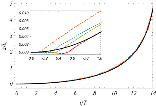
Figure 1: Center of mass drift in Schwarzschild spacetime for the cycle of Eq. (24), with $t_{0}/T=15$, $m_{0}/(m_{0}+3m_{1})=0.7$, and $m_{1}/(m_{0}+3m_{1})=0.1$. The vertical axis represents $z$, the tripod’s longitudinal displacement with respect to the reference geodesic, measured in units of $\ell_{0}$. The horizontal axis represents $t$, measured in units of the cycle period $T$. The phase parameter is set to $\chi=0$ (red curves, dash), $\chi=\pi/4$ (green curves, dash and single dot), $\chi=\pi/2$ (blue curves, dot), and $\chi=3\pi/4$ (orange curves, dash and double dots). The broken, colored curves are the result of numerical integrations, while the solid, black curves are the analytical approximation of Eqs. (35) and (37). A positive $z$ indicates that the tripod drifts upward, in the direction of increasing $R$ in the spacetime.

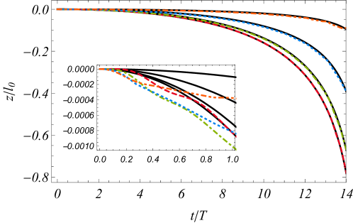
Figure 2: Same as Fig. 1 for the cycle of Eq. (27). Again we set $t_{0}/T=15$, $m_{0}/(m_{0}+3m_{1})=0.7$, and $m_{1}/(m_{0}+3m_{1})=0.1$. The phase parameter is set to $\chi=0$ (red curves, dash), $\chi=\pi/4$ (green curves, dash and single dot), $\chi=\pi/2$ (blue curves, dot), and $\chi=3\pi/4$ (orange curves, dash and double dots). The broken, colored curves are the result of numerical integrations, while the solid, black curves are the analytical approximation of Eq. (35), with the appropriate $\tilde{g}_{0}$ for this cycle evaluated at the corresponding $\chi$ ($\tilde{g}_{0}$ depends on $\chi$ for this cycle). A negative $z$ indicates that the tripod drifts downwards, in the direction of decreasing $R$ in the spacetime.

The analytical expression of Eqs. (35) and (37) allows us to calculate the tripod’s drift after one cycle of its internal motions. This is measured by $z(T)$, which evaluates to $\frac{1}{9}\tilde{g}_{0}(T/t_{0})^{2}$ after taking into account that $t_{0}\gg T$. Substituting Eq. (34) and relating $t_{0}^{-2}$ to the spacetime curvature through Eqs. (31) and (32), we write this as

$$z(T)=\frac{37}{9\pi}\frac{m_{0}m_{1}}{(m_{0}+3m_{1})^{2}}\,\ell_{0}^{2}\,(3\pi\ell_{0})\,\frac{GM}{R^{3}}.$$ (38)

We observe that the drift scales with $m_{0}m_{1}/(m_{0}+3m_{1})^{2}$, $\ell_{0}^{2}$, the area $3\pi\ell_{0}$ of the $\alpha$–$\ell$ plane swept out by the tripod’s cycle, and with the curvature $GM/R^{3}$. All these ingredients are also featured in Wisdom’s Eq. (20) wisdom:03 , and we therefore have recovered the essence of his result. We do not get a precise match — the numerical prefactor is different — because we adopt a different cycle for the tripod’s internal motions, model the struts in a slightly different way, and work in the Fermi frame of the free-falling observer instead of the static frame of the Schwarzschild spacetime.

As a final comment, it is interesting to note that the asymptotic relation (36), as $t$ approaches $t_{0}$, describes a geodesic of the Schwarzschild spacetime. Indeed, the homogeneous version of Eq. (23), $\ddot{z}+Bz=0$, is a component of the geodesic deviation equation, and its general solution

$$z_{\rm geo}(t)=\frac{1}{5}\bigl{[}4z(0)+3t_{0}\dot{z}(0)\bigr{]}(1-t/t_{0})^{-1/3}+\frac{1}{5}\bigl{[}z(0)-3t_{0}\dot{z}(0)\bigr{]}(1-t/t_{0})^{4/3}$$ (39)

describes a geodesic of the Schwarzschild spacetime that neighbors the reference geodesic $\gamma$. The first term dominates as $t$ approaches $t_{0}$, and we see that with

$$4z(0)+3t_{0}\dot{z}(0)=2\tilde{g}_{0},$$ (40)

$z_{\rm geo}$ becomes asymptotically equal to $z$. The world line described by Eq. (36), therefore, is a geodesic with initial conditions constrained by Eq. (40). This allows us to give an interpretation to the numerical results of Figs. 1 and 2. What we see is the tripod’s CM gradually transiting to a new geodesic described by Eq. (36) after being launched from the reference geodesic. The tripod is initially directed along $\gamma$, but the coupling between its internal motions and the spacetime curvature prevents it from following the reference geodesic. The motion is therefore nongeodesic for $0<t<t_{0}$, but it becomes increasingly geodesic as $t\to t_{0}$, that is, as the tripod approaches the curvature singularity at $R=0$. The approach to the singularity follows a geodesic, irrespective of the internal motions. The same reasoning can be applied to de Sitter spacetime, when a CM definition such that $g_{0}\neq 0$ is adopted. In this case, the motion asymptotes to $z\sim\frac{1}{2}g_{0}e^{2t/3t_{0}}$ when $t\gg t_{0}$, and this describes a geodesic of de Sitter spacetime with initial conditions constrained by $2z(0)+3t_{0}\dot{z}(0)=2g_{0}$.

IV.3 Conclusion

Our main conclusion in this section is that the motion of the tripod relative to the reference geodesic depends sensitively on the choice of internal cycle, but also on the choice of $\delta z_{0}$, the initial relativistic adjustment to the CM. The prescription advanced in Sec. III.2 left this quantity undetermined, and the prescription must therefore be completed by a choice of $\delta z_{0}$. A sensible (though not unique) option is to choose $\delta z_{0}$ so that $g_{0}=0$, thereby ensuring that a tripod placed in de Sitter spacetime does not drift away from the initial geodesic; this choice is motivated by the absence of a preferred direction in a maximally symmetric spacetime. Adopting the same CM when the tripod is placed in the Schwarzschild spacetime gives rise to a drift, with an approximate description given by Eqs. (35) and (37), in accordance to Wisdom’s original results wisdom:03 .

V Reconciliation with the Mathisson-Papapetrou-Dixon equations

The Mathisson-Papapetrou-Dixon (MPD) equations,

$$\frac{Dp_{\alpha}}{d\tau}=\frac{1}{2}S^{\mu\nu}u^{\lambda}R_{\mu\nu\lambda\alpha},\qquad\frac{DS_{\alpha\beta}}{d\tau}=2p_{[\alpha}u_{\beta]},$$ (41)

are meant to govern the motion of a generic extended body, in a pole-dipole approximation that neglects higher multipole moments but keeps the momentum vector $p_{\alpha}$ and spin tensor $S_{\alpha\beta}$; the velocity vector $u^{\alpha}$ is tangent to the world line, and $D/d\tau$ denotes a covariant derivative with respect to proper time $\tau$. Many derivations of these equations have been provided (see, for example, Refs. mathisson:10 ; papapetrou:51a ; bailey-israel:75 ), with the most comprehensive analysis supplied by Dixon dixon:70a ; dixon:70b ; dixon:74 . The puzzle that concerns us in this section is that while the MPD equations would be thought to adequately govern the motion of the tripod, the detailed examination carried out by Silva, Matsas, and Vanzella silva-matsas-vanzella:16 indicates that Eqs. (41) seem to be incompatible with the swimming motion described in Sec. IV.

One reason to suspect that Eqs. (41) may not apply to the tripod is that their derivation relies heavily on conservation of energy-momentum, as embodied by $\nabla_{\beta}T^{\alpha\beta}=0$, where $T^{\alpha\beta}$ is the energy-momentum tensor of the extended body. (Alternative derivations depend on the existence of a Lagrangian for the extended body, and this automatically enforces energy-momentum conservation.) The tripod, on the other hand, is a constrained mechanical system that does not conserve energy and momentum: the external agents responsible for the internal motions must supply energy and momentum to keep the tripod on its cycle.

This issue can be investigated by generalizing the Lagrangian-based derivation of Eqs. (41) provided by Bailey and Israel bailey-israel:80 to a constrained system. To showcase the modifications that result from the introduction of constraints, we consider the illustrative case of two particles moving freely in spacetime, except for a holonomic constraint that keeps their separation equal to a prescribed vector field $f^{\alpha}$. This is a covariant formulation of the type of tripod model introduced in Sec. III, and generalization to any number of particles (like four, for an actual tripod) is immediate.

Bailey and Israel place the two particles on physical world lines ${\cal P}_{1}$ and ${\cal P}_{2}$, but describe their motion in terms of a reference world line $\cal C$ that represents an arbitrary choice of “center of mass”. The world lines are given an arbitrary parameter $t$, the tangent vector to ${\cal C}$ is $u^{\alpha}$, and the separation between $\cal C$ and ${\cal P}_{A}$ at fixed $t$ is $-\sigma^{\alpha}_{A}$, with $A=1,2$ labelling the particle. The Lagrangian $L_{A}$ of each particle is the usual $-m_{A}d\tau_{A}/dt$ evaluated on ${\cal P}_{A}$, which is rewritten in terms of fields on ${\cal C}$; an explicit expression for the Lagrangian is given by their Eq. (76). The complete Lagrangian for the constrained system is $L=L_{1}+L_{2}+L_{\rm cons}$, with

$$L_{\rm cons}=\lambda_{\alpha}\bigl{(}\sigma^{\alpha}_{2}-\sigma^{\alpha}_{1}+f^{\alpha}\bigr{)},$$ (42)

where $\lambda_{\alpha}(t)$ is a Lagrange multiplier, and $f^{\alpha}(t)$ is the prescribed separation between the particles. The dynamical variables are defined by

$$p_{\alpha}:=\frac{\partial L}{\partial u^{\alpha}},\qquad S_{\alpha\beta}:=2\sigma_{1[\alpha}\frac{\partial L}{\partial\dot{\sigma}_{1}^{\beta]}}+2\sigma_{2[\alpha}\frac{\partial L}{\partial\dot{\sigma}_{2}^{\beta]}},$$ (43)

where $\dot{\sigma}^{\alpha}_{A}:=D\sigma_{A}^{\alpha}/dt$ is the covariant derivative of $\sigma^{\alpha}_{A}$ along ${\cal C}$.

Equations of motion for $p_{\alpha}$ and $S_{\alpha\beta}$ follow from the requirement that $S:=\int L\,dt$ be stationary under arbitrary variations of ${\cal P}_{A}$ and ${\cal C}$; the derivation also involves an identity deduced from the invariance of the action under an infinitesimal coordinate transformation. Variation with respect to ${\cal P}_{A}$ implicates the constraints, and Eq. (50) from bailey-israel:80 generalizes to

$$\frac{D}{dt}\frac{\partial L_{1}}{\partial\dot{\sigma}^{A}_{1}}-\frac{\partial L_{1}}{\partial\sigma^{\alpha}_{1}}=-\lambda_{\alpha},\qquad\frac{D}{dt}\frac{\partial L_{2}}{\partial\dot{\sigma}^{A}_{2}}-\frac{\partial L_{2}}{\partial\sigma^{\alpha}_{2}}=+\lambda_{\alpha};$$ (44)

these equations can be used to determine the Lagrange multiplier. Variation with respect to ${\cal C}$ reproduces Eq. (47) from bailey-israel:80 without change (we set the electric charge $e$ to zero), and their Eq. (51) acquires new terms coming from $L_{\rm cons}$.

Putting all this together, truncating the description of the motion to the pole-dipole approximation, and setting $t=\tau=\mbox{proper time on $\cal C$}$, we find that the equations of motion take the form of

$$\frac{Dp_{\alpha}}{d\tau}=\frac{1}{2}S^{\mu\nu}u^{\lambda}R_{\mu\nu\lambda\alpha},\qquad\frac{DS_{\alpha\beta}}{d\tau}=2p_{[\alpha}u_{\beta]}+2\lambda_{[\alpha}f_{\beta]},$$ (45)

which differ from Eqs. (41) by an additional torque term provided by the constraints. As expected, the original MPD equations do not apply to a constrained Lagrangian system.

Because Eqs. (45) are derived from a Lagrangian, they must be physically equivalent (after generalization to four particles, and approximation to weakly relativistic motion) to the equations of motion obtained in Sec. III, which also follow from a Lagrangian. To establish the equivalence explicitly would be difficult, because the two sets of equations implicate different variables, and because the constraints are implemented differently in each approach: in Sec. III the constraints were solved to express the Lagrangian in terms of the CM variables, while in this section they are enforced with Lagrange multipliers. Another obstacle toward establishing the equivalence of the two formulations is that Eqs. (45) remain empty of content until a relation between $p_{\alpha}$ and $u_{\alpha}$ is specified through the selection of a suitable “center of mass”; as we saw back in Sec. III, this can be a delicate matter. But in spite of these obstacles, we can be confident that Eqs. (22) or (23) and (45) describe the same system, because the two sets of equations originate from the same Lagrangian. In this admittedly incomplete way, we can reconcile Wisdom’s swimming with the MPD framework.

It seems to us that the selection of a “center of mass” is probably the most critical aspect of the comparison between Wisdom’s results wisdom:03 and the MPD framework; the additional terms in Eq. (45) may well be incidental. Indeed, we could imagine formulating a complete tripod model that includes all the springs and rubber bands that are dynamically responsible for the internal motions. Such a model could be described in terms of a Lagrangian or a conserved energy-momentum tensor, and such a tripod would be expected to satisfy Eqs. (41). But the selection of a “center of mass” for this model would be a delicate affair, and the precise relation between $p_{\alpha}$ and $u_{\alpha}$ might be complicated by the many details of the tripod’s design. For example, the choice of “center of mass” that comes with the oft-used covariant spin supplementary condition, $p_{\alpha}S^{\alpha\beta}=0$, might be entirely inadequate for such an object. In such circumstances, the relation between Eqs. (41) and the actual motion of the tripod might be very subtle and difficult to describe. This is another path of reconciliation.

References

- (1) J. Wisdom, Swimming in spacetime: Motion by cyclic changes in body shape, Science 299, 1865 (2003).
- (2) R. A. e. Silva, G. E. A. Matsas, and D. A. T. Vanzella, Rescuing the concept of swimming in curved spacetime, Phys. Rev. D 94, 121502 (2016), arXiv:1611.06183.
- (3) M. Mathisson, New mechanics of material systems (republication), Gen. Relativ. Gravit. 42, 1011 (2010).
- (4) A. Papapetrou, Spinning test-particles in general relativity. I, Proc. R. Soc. London, Ser. A 209, 248 (1951).
- (5) W. G. Dixon, Dynamics of extended bodies in general relativity. I. Momentum and angular momentum, Proc. Roy. Soc. London A314, 499 (1970).
- (6) W. G. Dixon, Dynamics of extended bodies in general relativity. II. Moments of the charge-current vector, Proc. Roy. Soc. London A319, 509 (1970).
- (7) W. G. Dixon, Dynamics of extended bodies in general relativity. III. Equations of motion, Phil. Trans. Roy. Soc. London A277, 59 (1974).
- (8) F. K. Manasse and C. W. Misner, Fermi normal coordinates and some basic concepts in differential geometry, J. Math. Phys. 4, 735 (1963).
- (9) E. Poisson, A. Pound, and I. Vega, The motion of point particles in curved spacetime, Living Rev. Rel. 14, 7 (2011), arXiv:1102.0529.
- (10) I. Bailey and W. Israel, Lagrangian dynamics of spinning particles and polarized media in general relativity, Commun. Math. Phys. 42, 65 (1975).
- (11) I. Bailey and W. Israel, Relativistic dynamics of extended bodies and polarized media: An eccentric approach, Ann. Phys. (N.Y.) 130, 188 (1980).