Baroclinically-driven flows and dynamo action
in rotating spherical fluid shells

Abstract

The dynamics of stably stratified stellar radiative zones is of considerable interest due to the availability of increasingly detailed observations of Solar and stellar interiors. This article reports the first non-axisymmetric and time-dependent simulations of flows of anelastic fluids driven by baroclinic torques in stably stratified rotating spherical shells – a system serving as an elemental model of a stellar radiative zone. With increasing baroclinicity a sequence of bifurcations from simpler to more complex flows is found in which some of the available symmetries of the problem are broken subsequently. The poloidal component of the flow grows relative to the dominant toroidal component with increasing baroclinicity. The possibility of magnetic field generation thus arises and this paper proceeds to provide some indications for self-sustained dynamo action in baroclinically-driven flows. We speculate that magnetic fields in stably stratified stellar interiors are thus not necessarily of fossil origin as it is often assumed.

1 Introduction

Stellar radiation zones are typically supposed to be motionless in standard models of stellar structure and evolution (Kippenhahn et al., 2012), but this assumption is poorly justified (Pinsonneault, 1997; Lebreton, 2000). Indeed, increasingly detailed evidence is emerging, e.g. from helio- and asteroseismology, of dynamical processes such as differential rotation, meridional circulation, turbulence, and internal waves in radiative zones (Turck-Chièze and Talon, 2008; Thompson et al., 2003; Gizon et al., 2010; Chaplin and Miglio, 2013; Aerts et al., 2010). These transport processes are important in mixing of angular momentum, evolution of chemical abundances, and magnetic field sustenance (Miesch and Toomre, 2009; Mathis, 2013). The problem of fluid motions in radiative zones is thus of wide significance.

Historically, this problem has been of much interest ever since it became apparent that rotating stellar interiors cannot be in a static equilibrium (von Zeipel, 1924), a statement known as von Zeipel’s paradox. Two different forms of flow have been hypothesized, namely (a) steady low-amplitude meridional circulations (Vogt, 1925; Eddington, 1925, 1925), and (b) particular forms of strong differential rotation with minimal meridional circulations (Schwarzschild, 1947; Roxburgh, 1964). It was demonstrated that hypothesis (a) is not an acceptable solution to von Zeipel’s paradox (Busse, 1981, 1982). Hypothesis (b) has since gained support with self-consistent quasi-one-dimensional solutions first derived by Zahn (1992) and their baroclinic instabilities studied (e.g. by Spruit and Knobloch, 1984; Caleo and Balbus, 2016). In recent years a number of numerical studies of axisymmetric and steady baroclinically-driven flows of finite amplitudes in rotating, stably stratified spherical shells have been published (Garaud, 2002; Rieutord, 2006; Espinosa and Rieutord, 2013; Hypolite and Rieutord, 2014; Rieutord and Beth, 2014). In (Garaud, 2002) the dynamics of the radiative zone of the Sun driven by the differential rotation of the convective zone is investigated, but the flow is essentially driven by the boundary conditions and baroclinicity is not the main driving force. The cited papers by Rieutord and coworkers offer perhaps the most detailed studies of the problem to date. However, the analysis is strongly restricted in two respects: first, two-dimensional and steady axisymmetric flows are studied, and second, the Boussinesq approximation is used which does not account for the strong density variations typical for stably stratified regions of stars.

In this paper we present a model of baroclinic flows in rotating spherical fluid shells. The model is based on the anelastic approximation (Gough, 1969; Braginsky and Roberts, 1995; Lantz and Fan, 1999) of the fully-compressible fluid equations which is widely adopted for numerical simulation of convection in Solar and stellar interiors (Jones et al., 2011). While this approximation is strictly only valid for a system close to an adiabatic state it, nevertheless, relaxes the assumptions of the Boussinesq approximation that has been used previously. In the basic state the density is stably stratified in the radial direction and axisymmetric shear driven motions are realized. Starting with this basic axisymmetric baroclinic state we explore the onset of non-axisymmetric and time dependent states and investigate their nonlinear properties. Further, we consider the possibility of magnetic field generation by these flows. Although a prime motivation for our study is to understand the motions in stellar radiative zones, we have not strived to adjust the values of the dimensionless parameters in our model to physically realistic ones. This is not possible in any case since the Reynolds number of flows in stars is huge and turbulent mixing occurs. Only the large scale flows can be simulated numerically while the influence of turbulence is taken into account through the use of eddy diffusivities in the equations of motion. For details of this approach we refer to the work of Miesch and Toomre (2009) and references therein. Using this approach we shall overcome the restrictions of axisymmetric steady flows which are likely to be unstable. As we shall show non-axisymmetric and time dependent flows must be expected instead with properties that could give rise to dynamo action.

2 Mathematical model

We consider a perfect gas confined to a spherical shell rotating with a fixed angular velocity $\varOmega\hat{\mbox{\boldmath$k$}}$ and with a positive entropy contrast $\Delta S$ imposed between its outer and inner surfaces at radii $r_{o}$ and $r_{i}$, respectively. We assume a gravity field proportional to $g/r^{2}$. To justify this choice consider the Sun, the star with the best-known physical properties. The Solar density drops from 150 g/cm³ at the centre to 20 g/cm³ at the core-radiative zone boundary (at $0.25R_{\odot}$) to only 0.2 at the tachocline (at $0.7R_{\odot}$). A crude piecewise linear interpolation shows that most of the mass is concentrated within the core. In this setting a hydrostatic polytropic reference state exists with profiles of density $\bar{\rho}=\rho_{c}\zeta^{n}$, temperature $\bar{T}=T_{c}\zeta$ and pressure $\bar{P}=P_{c}\zeta^{n+1}$, where $\zeta=c_{0}+c_{1}/r$ and $c_{0}=(2\zeta_{o}-\eta-1)/(1-\eta)$, $c_{1}=(1+\eta)(1-\zeta_{o})/(1-\eta)^{2}$, $\zeta_{o}=(\eta+1)/(\eta\exp(N_{\rho}/n)+1)$, see (Jones et al., 2011). The parameters $\rho_{c}$, $P_{c}$ and $T_{c}$ are reference values of density, pressure and temperature at mid-shell. The gas polytropic index $n$, the density scale height $N_{\rho}$ and the shell radius ratio $\eta$ are defined further below. Following Rieutord (2006) we neglect the distortion of the isopycnals caused by the centrifugal force. The governing anelastic equations of continuity, momentum and energy (entropy) take the

form

$${\bm\nabla}{\bm\cdot}\bar{\rho}\mbox{\boldmath$u$}= 0,$$ (1a)

$$\upartial_{t}\mbox{\boldmath$u$}+({\bm\nabla}\times\mbox{\boldmath$u$})\times\mbox{\boldmath$u$}= -{\bm\nabla}\varPi-\tau(\hat{\mbox{\boldmath$k$}}\times\mbox{\boldmath$u$})+\frac{\mathrm{R}}{\mathrm{Pr}}\frac{{S}}{r^{2}}\hat{\mbox{\boldmath$r$}}+\mbox{\boldmath$F$}_{\nu}$$

$$\qquad\quad-{\mathrm{Z}}(\overline{S}+S)\;\hat{\mbox{\boldmath$k$}}\times(\mbox{\boldmath$r$}\times\hat{\mbox{\boldmath$k$}}),$$ (1b)

$$\upartial_{t}S+\mbox{\boldmath$u$}{\bm\cdot}{\bm\nabla}{(\overline{S}+S)}= \frac{1}{\mathrm{Pr}\bar{\rho}\bar{T}}{\bm\nabla}{\bm\cdot}\bar{\rho}\bar{T}{\bm\nabla}S+{\frac{c_{1}\mathrm{Pr}}{\mathrm{R}\bar{T}}Q_{\nu}},$$ (1c)

where $S$ is the deviation from the background entropy profile $\overline{S}=(\zeta(r)^{-n}-\zeta_{o}^{-n})/(\zeta_{o}^{-n}-\zeta_{i}^{-n})$ and $u$ is the velocity vector, ${\bm\nabla}\varPi$ includes all terms that can be written as gradients, and $\mbox{\boldmath$r$}=r\hat{\mbox{\boldmath$r$}}$ is the position vector with respect to the center of the sphere (Jones et al., 2011; Simitev et al., 2015). The viscous force $\mbox{\boldmath$F$}_{\nu}=(\rho_{c}/\bar{\rho}){\bm\nabla}{\bm\cdot}\mbox{\boldmath$\hat{S}$}$ and the viscous heating $Q_{\nu}=\mbox{\boldmath$\hat{S}$}{\bm:}\mbox{\boldmath$e$}$ are defined in terms of the deviatoric stress tensor $\hat{S}_{ij}=2\bar{\rho}(e_{ij}-e_{kk}\delta_{ij}/3)$ with $e_{ij}=(\upartial_{i}u_{j}+\upartial_{j}u_{i})/2$, where double-dots (:) denote a Frobenius inner product, and $\nu$ is a constant viscosity. The governing equations (1) have been non-dimensionalized with the shell thickness $d=r_{o}-r_{i}$ as unit of length, $d^{2}/\nu$ as unit of time, and $\Delta S$, $\rho_{c}$ and $T_{c}$ as units of entropy, density and temperature, respectively. The system is then characterized by seven dimensionless parameters: the radius ratio $\eta=r_{i}/r_{o}$, the polytropic index of the gas $n$, the density scale number $N_{\rho}=\ln\big{(}\bar{\rho}(r_{i})/\bar{\rho}(r_{o})\big{)}$, the Prandtl number $\mathrm{Pr}={\nu}/{\kappa}$, the Rayleigh number $\mathrm{R}=-{gd^{3}\Delta S}/({\nu\kappa c_{p}})$, the baroclinicity parameter ${\mathrm{Z}}={\varOmega^{2}d^{4}\Delta S}/({\nu^{2}c_{p}})$, and the Coriolis number $\tau={2\varOmega d^{2}}/{\nu}$, where $\kappa$ is a constant entropy diffusivity and $c_{p}$ is the specific heat at constant pressure. Note, that the Rayleigh number assumes negative values in the present problem since the basic entropy gradient is reversed with respect to the case of buoyancy driven convection. The poloidal-toroidal decomposition

$$\bar{\rho}\mbox{\boldmath$u$}={\bm\nabla}\times({\bm\nabla}\times\hat{\mbox{\boldmath$r$}}rv)+{\bm\nabla}\times\hat{\mbox{\boldmath$r$}}r^{2}w$$

is used to enforce the solenoidality of the mass flux $\bar{\rho}\mbox{\boldmath$u$}$. This has the further advantages that the pressure gradient is eliminated and scalar equations for the poloidal and the toroidal scalar fields, $v$ and $w$, are obtained by taking $\hat{\mbox{\boldmath$r$}}{\bm\cdot}{\bm\nabla}{\times{\bm\nabla}\times}$ and $\hat{\mbox{\boldmath$r$}}{\bm\cdot}{\bm\nabla}\times$ of equation (1b). Except for the term with the baroclinicity parameter ${\mathrm{Z}}$ the resulting equations are identical to those described by Simitev et al. (2015). Assuming that entropy fluctuations are damped by convection in the region above $r=r_{o}$ we choose the boundary condition

$$S =0\;\; \text{at }\qquad r =\left\{\begin{array}[]{l}r_{i}\equiv\eta/(1-\eta)\,,\\[1.00006pt] r_{o}\equiv 1/(1-\eta)\,,\end{array}\right.\qquad$$ (2c)

while the inner and the outer boundaries of the shell are assumed stress-free and impenetrable for the flow

$$v=0,\quad\upartial_{r}^{2}v=\frac{\bar{\rho}^{\prime}}{\bar{\rho}r}\upartial_{r}{}(rv),\quad\upartial_{r}(rw) =\frac{\bar{\rho}^{\prime}}{\bar{\rho}}w\; \text{at }\qquad r =\left\{\begin{array}[]{l}r_{i}\,,\\[1.00006pt] r_{o}\,.\end{array}\right.$$ (2f)

3 Numerical solution

For the numerical solution of problem (1–2) a pseudo-spectral method described by Tilgner (1999) was employed. A code developed and used by us for a number of years (Busse et al., 2003; Busse and Simitev, 2011; Simitev et al., 2015) and extensively benchmarked for accuracy (Simitev et al., 2015; Marti et al., 2014; Matsui et al., 2016) was adapted. Adequate numerical resolution for the runs has been chosen as described in (Simitev et al., 2015). To analyse the properties of the solutions we decompose the kinetic energy density into poloidal and toroidal components and further into mean (axisymmetric) and fluctuating (nonaxisymmetric) components and into equatorially-symmetric and equatorially-antisymmetric components,

$$\overline{E}_{p}=\overline{E}_{p}^{s}+\overline{E}_{p}^{a} =\langle\big{(}{\bm\nabla}\times({\bm\nabla}\bar{v}\times\mbox{\boldmath$r$})\big{)}^{2}/(2\bar{\rho})\rangle,$$

$$\overline{E}_{t}=\overline{E}_{t}^{s}+\overline{E}_{t}^{a} =\langle\big{(}{\bm\nabla}r\bar{w}\times\mbox{\boldmath$r$}\big{)}^{2}/(2\bar{\rho})\rangle,$$

$$\widetilde{E}_{p}=\widetilde{E}_{p}^{s}+\widetilde{E}_{p}^{a} =\langle\big{(}{\bm\nabla}\times({\bm\nabla}\check{v}\times\mbox{\boldmath$r$})\big{)}^{2}/(2\bar{\rho})\rangle,$$

$$\widetilde{E}_{t}=\widetilde{E}_{t}^{s}+\widetilde{E}_{t}^{a} =\langle\big{(}{\bm\nabla}r\check{w}\times\mbox{\boldmath$r$}\big{)}^{2}/(2\bar{\rho})\rangle,$$

where angular brackets $\langle\,\,\rangle$ denote averages over the volume of the spherical shell.

4 Parameter values and initial conditions

In the simulations presented here fixed values are used for all governing parameters except for the baroclinicity ${\mathrm{Z}}$ namely $\eta=0.3$, $n=2$, $N_{\rho}=2$, $\mathrm{Pr}=0.1$, $\tau=300$ and $\mathrm{R}=-5\times 10^{4}$. The value for the shell thickness represents the presence of a stellar core geometrically similar to that of the Sun. The values for $n$ and $N_{\rho}$ are not far removed from estimates $n=1.5$ and $N_{\rho}=4.6052$ for the solar radiative zone.

The strength of the baroclinic forcing, measured by ${\mathrm{Z}}$, is limited from above so that

$${\mathrm{Z}}<(1-\eta)^{3}\;|\mathrm{R}|/\mathrm{Pr}.$$

This restriction guarantees that the apparent gravity does not point outward such that the model excludes standard thermal convection instabilities.

Unresolved subgrid-scales in convective envelopes are typically modelled by the assumption of approximately equal turbulent eddy diffusivities and the choice of $\mathrm{Pr}=1$ is often made in the literature (Miesch et al., 2015). However, in the presence of the minute Prandtl number values based on molecular diffusivities the eddy diffusivities are not likely to yield an effective Prandtl number of the order unity. Furthermore, in a stably stratified system turbulence is expected to be anisotropic (Zahn, 1992). With this in mind we have chosen $\mathrm{Pr}=0.1$ in our study.

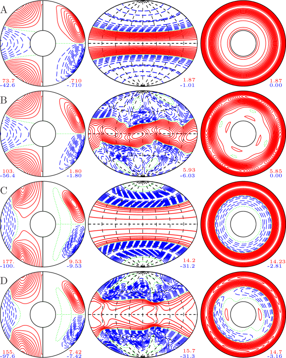
Figure 1: Flow structures with increasing baroclinicity ${\mathrm{Z}}\times 10^{-4}=7$, $10$, $14$ and $14$ from top to bottom. Bistability occurs at ${\mathrm{Z}}\times 10^{-4}=14$. The values of the other parameters are $\eta=0.3$, $n=2$, $N_{\rho}=2$, $\mathrm{Pr}=0.1$, $\tau=300$ and $\mathrm{R}=-5\times 10^{4}$. The first plot in each row shows isocontours of $\overline{u}_{\varphi}$ (left half) and streamlines $r\sin\theta(\upartial_{\theta}\overline{v})=$ const. (right half) in the meridional plane. The second plot shows isocontours of $u_{r}$ at $r=r_{i}+0.7$. The third plot shows isocontours of $u_{r}$ in the equatorial plane. The minimal and the maximal values of each field are listed under the corresponding plot; The isocontours are equidistant with positive isocontours shown by solid lines, negative isocontours shown by broken lines and the zeroth isocontour shown by a dotted line in each plot. (Colour online)

The value $\tau=300$ offers a good compromise in which the effect of rotation is strong enough to govern the dynamics of the system, but not too strong to cause a significant increase of the computational expenses; similar values are used e.g. by Simitev et al. (2015) and in cases F1–4 of (Käpylä et al., 2016). A negative $\mathrm{R}=-5\times 10^{4}$ is assumed to model a convectively stable situation.

Initial conditions of no fluid motion are used at vanishingly small values of ${\mathrm{Z}}$, while at finite values of ${\mathrm{Z}}$ the closest equilibrated neighbouring case is used as initial condition to help convergence and reduce transients. To ensure that transient effects are eliminated from the sequence presented below, all solutions have been continued for at least 15 time units.

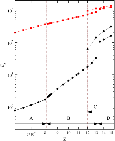
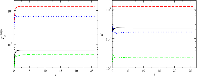
Figure 2: Time-averaged kinetic energy densities as functions of baroclinicity ${\mathrm{Z}}$ for $\eta=0.3$, $n=2$, $N_{\rho}=2$, $\mathrm{Pr}=0.1$, $\tau=300$ and $\mathrm{R}=-5\times 10^{4}$. Full and empty symbols indicate equatorially-symmetric and -asymmetric energy components, respectively. Black circles, red squares, green triangles-up and blue triangles-down indicate the energy components $\overline{E}_{p}^{s,a}$, $\overline{E}_{t}^{s,a}$, $\widetilde{E}_{p}^{s,a}$, $\widetilde{E}_{t}^{s,a}$, respectively. Axially-symmetric and axially-asymmetric components are plotted in the left and the right panels, respectively. Vertical dash-dotted lines indicate transition points. The ranges over which the four distinct states are observed are indicated by arrows near the bottom abscissa, with states B and C and D and C co-existing as shown. Energy components not shown are at least 10 orders of magnitude smaller than the ones shown. (Colour online)

Figure 3: Time series of magnetic dipolar energy densities (left panel) and equatorially-symmetric kinetic energy densities (right pannel) in the dynamo case ${\mathrm{Z}}=17\times 10^{4}$, $\mathrm{Pm}=16$, for $\eta=0.3$, $n=2$, $N_{\rho}=2$, $\mathrm{Pr}=0.1$, $\tau=300$ and $\mathrm{R}=-5\times 10^{4}$. Black solid lines, red dashed lines, green dash-dotted lines and blue dotted lines indicate the components $\overline{E}_{p}^{s}$, $\overline{E}_{t}^{s}$, $\widetilde{E}_{p}^{s}$, $\widetilde{E}_{t}^{s}$, and the corresponding dipolar magnetic components, respectively. All other energy density components are smaller by more than 5 orders of magnitude. (Colour online)

5 Baroclinic flow instabilities

The baroclinically-driven problem is invariant under a group of symmetry operations including rotations about the polar axis i.e. invariance with respect to the coordinate transformation $\varphi\to\varphi+\alpha$, reflections in the equatorial plane $\theta\to\pi-\theta$, and translations in time $t\to t+a$, see (Gubbins and Zhang, 1993). As baroclinicity ${\mathrm{Z}}$ is increased the available symmetries of the solution are broken resulting in a sequence of states ranging from simpler and more symmetric flow patterns to more complex flow patterns of lesser symmetry as illustrated in figure 1. In this respect the system resembles Rayleigh-Benard convection (Busse, 2003). The sequence starts with the basic axisymmetric, equatorially symmetric and time-independent state with a dominant wave number $k=1$ in the radial direction labelled A in figures 1 and 3. An instability occurs at about ${\mathrm{Z}}=8.1\times 10^{4}$ leading to a state B characterized by a dominant azimuthal wavenumber $m=2$ in the expansion of the solution in spherical harmonics $Y_{l}^{m}$, i.e. while the full axisymmetry is broken, a symmetry holds with respect to the transformation $\varphi\to\varphi+\pi$. Simultaneously, the symmetry about the equatorial plane is also broken in state B. At ${\mathrm{Z}}=13.25\times 10^{4}$ a further transition to a pattern labelled D occurs. While state D continues to have a $m=2$ azimuthal symmetry, the symmetry about the equatorial plane is now restored. In addition, a dominant radial wave number $k=2$ develops as is evident, for instance, from the concentric two-roll meridional circulation in state D. Remarkably, both states B and D coexist with a steady pattern C that can be found for the range of values ${\mathrm{Z}}>12\times 10^{4}$. State C is axisymmetric, equatorially symmetric and time-independent but differs from state A in that it keeps a dominant radial wave number $k=2$. Which one of the coexisting branches will be found in a given numerical simulation is determined by the specific initial conditions used. While all patterns in the sequence presented here remain time-independent in their respective drifting frames of reference, we expect that time-dependent solutions will be found for lower values of the Prandtl number since the Reynolds number is increasing at a fixed baroclinicity ${\mathrm{Z}}$ and as a result breaking of additional symmetries is likely to occur.

The bifurcations and their abrupt nature are also evident in figure 3 where the time-averaged kinetic energy densities are plotted with increasing baroclinicity ${\mathrm{Z}}$. At ${\mathrm{Z}}=0$ all energies vanish corresponding to the state of rigid body rotation with vanishing velocity field. In the range ${\mathrm{Z}}<6\times 10^{4}$ velocities grow linearly with ${\mathrm{Z}}$ and the corresponding growth of kinetic energies is well described by the empirical relations

$$\overline{E}_{t}^{s}=5.647\times 10^{-8}\;{\mathrm{Z}}^{2},\qquad\qquad\overline{E}_{p}^{s}=2.377\times 10^{-10}\;{\mathrm{Z}}^{2},$$

indicating the dominance of toroidal motions as argued in earlier theoretical analyses (Busse, 1981, 1982; Zahn, 1992). While the particular numerical factors in these expressions depend on the parameter values used, the quadratic form of this dependence is expected to be generic. The abrupt jumps in energies at intermediate values of ${\mathrm{Z}}$ correspond to the breaking of spatial symmetries. In state A, for instance, only the axially-symmetric poloidal (i.e. meridional circulation) and toroidal (i.e. differential rotation) kinetic energies have non negligible values. In state B the non-axisymmetric components emerge with the equatorially asymmetric ones being larger than the corresponding equatorially symmetric ones. In state D equatorially asymmetric components become negligible again and in state C all non-axisymmetric energy components decay. In the regions of hysteretic bistability $12\times 10^{4}<{\mathrm{Z}}<13.25\times 10^{4}$ and ${\mathrm{Z}}>13.25\times 10^{4}$ either of states B or C or states D or C may be realized, respectively, depending on initial conditions.

6 Baroclinic dynamos

Approximately 10% of intermediate-mass and massive stars which are mainly radiative are known to be magnetic (Donati and Landstreet, 2009). The most popular hypothesis is that these are fossil fields remnants of an early phase of the stellar evolution (Donati and Landstreet, 2009). The possibility of dynamos generated in stably stratified stellar radiation regions has received only limited support in the literature (e.g. Braithwaite, 2006), because it is well known that dynamo action does not exist in a spherical system in the absence of a radial component of motion (Bullard and Gellman, 1954). The latter is, indeed, rather weak in the basic state A of low poloidal kinetic energy as discussed above. However, with increasing baroclinicity ${\mathrm{Z}}$, the growing radial component of the velocity field strengthens the probability of dynamo action.

To investigate this possibility the Lorentz force $(1/\bar{\rho})({\bm\nabla}\times\mbox{\boldmath$B$})\times\mbox{\boldmath$B$}$ has been added to the right-hand side of equation (1b) and the equation of magnetic induction

$$\upartial_{t}\mbox{\boldmath$B$}={\bm\nabla}\times(\mbox{\boldmath$u$}\times\mbox{\boldmath$B$})+\mathrm{Pm}^{-1}\nabla^{2}\mbox{\boldmath$B$},$$

has been added to equations (1) to attain the full magnetohydrodynamic form as used in the works of Jones et al. (2011) and Simitev et al. (2015). Here, $B$ is the magnetic flux density and $\mathrm{Pm}={\nu}/{\lambda}$ is the magnetic Prandtl number with $\lambda$ being the magnetic diffusivity. After adding vanishingly small random magnetic fields as initial conditions to equilibrated purely hydrodynamic solutions, a number of solutions with growing magnetic fields of dipolar character have been obtained. As an example, figures 3 and 4 demonstrate the magnetic field generated at ${\mathrm{Z}}=17\times 10^{4}$ and for the magnetic Prandtl number $\mathrm{Pm}=16$ which has been started from an equilibrated neighbouring case to help convergence and reduce transients. The dynamo solution quickly attains a stationary state that we have followed for nearly 2 magnetic diffusion time units, $t/\mathrm{Pm}$, as shown in figure 3. The ratio of poloidal to toroidal magnetic energy is $E_{p}^{\text{magn}}/E_{t}^{\text{magn}}=0.059$ and the ratio of magnetic to kinetic total energy is $E^{\text{magn}}/E^{\text{kin}}=0.127$. Furthermore, the energy density of the magnetic field $E^{\text{magn}}$ is comparable to the kinetic energy density of the poloidal component of the velocity field, $E_{p}^{\text{kin}}$. The magnetic field has a negligible quadrupolar component and a large-scale dipolar topology shown in figure 4 that does not change in time, resembling in this respect the surface fields of Ap-Bp stars (Donati and Landstreet, 2009). The surface structure of the magnetic field is characterised by two prominent patches of opposite polarity situated at approximately $45^{\circ}$ in latitude. The azimuthally-averaged toroidal field shows a pair of hook-shaped toroidal flux tubes largely filling the outer layer of the shell at lower latitudes as well as a pair of toroidal flux tubes in the polar regions and parallel to the rotation axis. While a large scale dipolar component emerges outside of the spherical shell, the azimuthally-averaged poloidal field also shows a pair of octupole poloidal flux tubes confined to the interior of the shell. Azimuthally-averaged kinetic and magnetic helicities are plotted in the last column of figure 4. These latter quantities are important in modelling the electromotive force in mean-field dynamo theories, and in estimating the topological linkage of magnetic field lines, respectively.

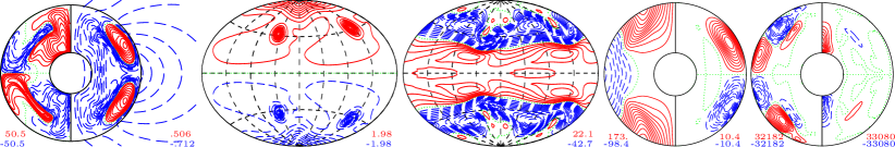
Figure 4: A dynamo solution at ${\mathrm{Z}}=17\times 10^{4}$ and $\mathrm{Pm}=16$ for $\eta=0.3$, $n=2$, $N_{\rho}=2$, $\mathrm{Pr}=0.1$, $\tau=300$ and $\mathrm{R}=-5\times 10^{4}$. corresponding to the end of time in Figure 3. The first plot shows isocontours of $\overline{B}_{\varphi}$ (left half) and meridional field lines $r\sin\theta\,\upartial_{\theta}\bar{h}=$ const. (right half). The second plot shows isocontours of radial magnetic field ${B}_{r}$ at $r=r_{o}+0.1$. The third plot shows isocontours of radial velocity $u_{r}$ at $r=r_{i}+0.7$. The fourth plot shows isocontours of $\overline{u}_{\varphi}$ (left half) and streamlines $r\sin\theta(\upartial_{\theta}\overline{v})=$ const. (right half) in the meridional plane. The last plot shows isocontours of azimuthally-averaged kinetic helicity $\overline{\mbox{\boldmath$u$}{\bm\cdot}{\bm\nabla}\times\mbox{\boldmath$u$}}$ (left half) and magnetic helicity $\overline{\mbox{\boldmath$B$}{\bm\cdot}{\bm\nabla}\times\mbox{\boldmath$B$}}$ (right half) in the meridional plane. Minimal and maximal values and isocontour line types are denoted following the convention of Figure 1. (Colour online)

7 Conclusion

In summary, we have described the bifurcations leading to non-axisymmetric and non-equatorially symmetric flow states with increasing baroclinicity. The observed sequence of baroclinic instabilities is rather different from the typical sequence of convective instabilities familiar from the literature (e.g. Sun et al., 1993; Simitev and Busse, 2003). Furthermore, we have demonstrated the possibility of dynamo action in baroclinically-driven flows. We remark that the details of the bifurcation sequence depend on the choice of parameter values. But preliminary additional computations indicate that the general picture described here persists when parameter values are changed by up to a factor of 10. While the dynamo solution discussed above is obtained for an unphysically large value of the magnetic Prandtl number, we argue that magnetic fields in stably stratified stellar interiors may not necessarily be of fossil origin as often assumed and that dynamo action may possibly occur in the radiative zones of rotating stars. Even in the solar interior below the convection zone magnetic fields may be generated. This possibility has not yet been investigated as far as we know.

References

- Aerts et al. (2010) Aerts, C., Christensen-Dalsgaard, J. and Kurtz, D., Asteroseismology, 2010 (Springer).
- Braginsky and Roberts (1995) Braginsky, S. and Roberts, P., Equations governing convection in earth’s core and the geodynamo. Geophys. Astrophys. Fluid Dyn., 1995, 79, 1–97.
- Braithwaite (2006) Braithwaite, J., A differential rotation driven dynamo in a stably stratified star. Astron. & Astrophys., 2006, 449, 451–460.
- Bullard and Gellman (1954) Bullard, E. and Gellman, H., Homogeneous dynamos and terrestrial magnetism. Phil. Trans. R. Soc. A, 1954, 247, 213–278.
- Busse (1981) Busse, F., Do Eddington-Sweet circulations exist?. Geophys. Astrophys. Fluid Dyn., 1981, 17, 215–235.
- Busse (1982) Busse, F., On the problem of stellar rotation. Astrophys. J., 1982, 259, 759–766.
- Busse (2003) Busse, F., The sequence-of-bifurcations approach towards understanding turbulent fluid flow. Surv. Geophys., 2003, 24, 269–288.
- Busse et al. (2003) Busse, F., Grote, E. and Simitev, R., Convection in rotating spherical shells and its dynamo action. In Earth’s Core and Lower Mantle, edited by C. Jones, A. Soward and K. Zhang, pp. 130–152, 2003 (Taylor & Francis: London & New York).
- Busse and Simitev (2011) Busse, F. and Simitev, R., Remarks on some typical assumptions in dynamo theory. Geophys. Astrophys. Fluid Dyn., 2011, 105, 234.
- Caleo and Balbus (2016) Caleo, A. and Balbus, S., The radiative zone of the Sun and the tachocline: stability of baroclinic patterns of differential rotation. Mon. Not. R. Astron. Soc., 2016, 457, 1711–1721.
- Chaplin and Miglio (2013) Chaplin, W. and Miglio, A., Asteroseismology of solar-type and red-giant stars. Annu. Rev. Astron. Astrophys., 2013, 51, 353–392.
- Donati and Landstreet (2009) Donati, J.F. and Landstreet, J., Magnetic fields of nondegenerate stars. Annu. Rev. Astron. Astrophys., 2009, 47, 333–370.
- Eddington (1925) Eddington, A., A limiting case in the theory of radiative equilibrium. Mon. Not. R. Astron. Soc., 1925, 85, 408.
- Eddington (1925) Eddington, A., Circulating currents in rotating stars. The Observatory, 1925, 48, 73–75.
- Espinosa and Rieutord (2013) Espinosa, L. and Rieutord, M., Self-consistent 2D models of fast-rotating early-type stars. Astron. Astrophys., 2013, 552, A35.
- Garaud (2002) Garaud, P., On rotationally driven meridional flows in stars. Mon. Not. R. Astron. Soc., 2002, 335, 707–711.
- Gizon et al. (2010) Gizon, L., Birch, A. and Spruit, H., Local helioseismology: Three-dimensional imaging of the solar interior. Annu. Rev. Astron. Astrophys., 2010, 48, 289–338.
- Gough (1969) Gough, D., The anelastic approximation for thermal convection. J. Atmos. Sci., 1969, 26, 448.
- Gubbins and Zhang (1993) Gubbins, D. and Zhang, K., Symmetry properties of the dynamo equations for palaeomagnetism and geomagnetism. Phys. Earth Planet. Inter., 1993, 75, 225 – 241.
- Hypolite and Rieutord (2014) Hypolite, D. and Rieutord, M., Dynamics of the envelope of a rapidly rotating star or giant planet in gravitational contraction. Astron. Astrophys., 2014, 572, A15.
- Jones et al. (2011) Jones, C., Boronski, P., Brun, A., Glatzmaier, G., Gastine, T., Miesch, M. and Wicht, J., Anelastic convection-driven dynamo benchmarks. Icarus, 2011, 216, 120 – 135.
- Käpylä et al. (2016) Käpylä, P.J., Käpylä, M.J., Olspert, N., Warnecke, J. and Brandenburg, A., Convection-driven spherical shell dynamos at varying Prandtl numbers. Astron. Astrophys., 2016, 10.1051/aas:1997209.
- Kippenhahn et al. (2012) Kippenhahn, R., Weigert, A. and Weiss, A., Stellar Structure and Evolution, 2012 (Springer).
- Lantz and Fan (1999) Lantz, S. and Fan, Y., Anelastic magnetohydrodynamic equations for modeling solar and stellar convection zones. Astrophys. J. Suppl. Ser., 1999, 121, 247.
- Lebreton (2000) Lebreton, Y., Stellar structure and evolution: Deductions from Hipparcos. Annu. Rev. Astron. Astrophys., 2000, 38, 35–77.
- Marti et al. (2014) Marti, P., Schaeffer, N., Hollerbach, R., Cébron, D., Nore, C., Luddens, F., Guermond, J.L., Aubert, J., Takehiro, S., Sasaki, Y., Hayashi, Y.Y., Simitev, R., Busse, F., Vantieghem, S. and Jackson, A., Full sphere hydrodynamic and dynamo benchmarks. Geophys. J. Int., 2014, 197, 119–134.
- Mathis (2013) Mathis, S., Transport processes in stellar interiors. In Studying Stellar Rotation and Convection: Theoretical Background and Seismic Diagnostics, edited by M. Goupil, K. Belkacem, C. Neiner, F. Lignières and J.J. Green, pp. 23–47, 2013 (Springer: Berlin, Heidelberg).
- Matsui et al. (2016) Matsui, H., Heien, E., Aubert, J., Aurnou, J.M., Avery, M., Brown, B., Buffett, B.A., Busse, F., Christensen, U.R., Davies, C.J., Featherstone, N., Gastine, T., Glatzmaier, G.A., Gubbins, D., Guermond, J.L., Hayashi, Y.Y., Hollerbach, R., Hwang, L.J., Jackson, A., Jones, C.A., Jiang, W., Kellogg, L.H., Kuang, W., Landeau, M., Marti, P.H., Olson, P., Ribeiro, A., Sasaki, Y., Schaeffer, N., Simitev, R.D., Sheyko, A., Silva, L., Stanley, S., Takahashi, F., Takehiro, S.I., Wicht, J. and Willis, A.P., Performance benchmarks for a next generation numerical dynamo model. Geochem. Geophys. Geosys., 2016, 17, 1586–1607.
- Miesch and Toomre (2009) Miesch, M. and Toomre, J., Turbulence, magnetism, and shear in stellar interiors. Annu. Rev. Fluid Mech., 2009, 41, 317–345.
- Miesch et al. (2015) Miesch, M., Matthaeus, W., Brandenburg, A., Petrosyan, A., Pouquet, A., Cambon, C., Jenko, F., Uzdensky, D., Stone, J., Tobias, S., Toomre, J. and Velli, M., Large-eddy simulations of magnetohydrodynamic turbulence in heliophysics and astrophysics. Space Sci. Rev., 2015, 194, 97–137.
- Pinsonneault (1997) Pinsonneault, M., Mixing in stars. Annu. Rev. Astron. Astrophys., 1997, 35, 557–605.
- Rieutord (2006) Rieutord, M., The dynamics of the radiative envelope of rapidly rotating stars. Astron. Astrophys., 2006, 451, 1025–1036.
- Rieutord and Beth (2014) Rieutord, M. and Beth, A., Dynamics of the radiative envelope of rapidly rotating stars: Effects of spin-down driven by mass loss. Astron. Astrophys., 2014, 570, A42.
- Roxburgh (1964) Roxburgh, I., On stellar rotation, I. The rotation of upper main-sequence stars. Mon. Not. R. Astron. Soc., 1964, 128, 157.
- Schwarzschild (1947) Schwarzschild, M., On stellar rotation. Astrophys. J., 1947, 106, 427.
- Simitev and Busse (2003) Simitev, R. and Busse, F., Patterns of convection in rotating spherical shells. New J. Phys., 2003, 5, 97.
- Simitev et al. (2015) Simitev, R., Kosovichev, A. and Busse, F., Dynamo effects near the transition from solar to anti-solar differential rotation. Astrophys. J., 2015, 810, 80.
- Spruit and Knobloch (1984) Spruit, H. and Knobloch, E., Baroclinic instability in stars. Astron. Astrophys., 1984, 132, 89–96.
- Sun et al. (1993) Sun, Z., Schubert, G. and Glatzmaier, G., Transitions to chaotic thermal convection in a rapidly rotating spherical fluid shell. Geophys. Astrophys. Fluid Dyn., 1993, 69, 95–131.
- Thompson et al. (2003) Thompson, M.J., Christensen-Dalsgaard, J., Miesch, M.S. and Toomre, J., The Internal Rotation of the Sun. Annu. Rev. Astron. Astrophys., 2003, 41, 599–643.
- Tilgner (1999) Tilgner, A., Spectral methods for the simulation of incompressible flows in spherical shells. Int. J. Numer. Meth. Fluids, 1999, 30, 713–724.
- Turck-Chièze and Talon (2008) Turck-Chièze, S. and Talon, S., The dynamics of the solar radiative zone. Adv. Space Res., 2008, 41, 855–860.
- Vogt (1925) Vogt, H., Zum Strahlungsgleichgewicht der Sterne. Astron. Nachr., 1925, 223, 229.
- von Zeipel (1924) von Zeipel, H., The radiative equilibrium of a rotating system of gaseous masses. Mon. Not. R. Astron. Soc., 1924, 84, 665–683.
- Zahn (1992) Zahn, J.P., Circulation and turbulence in rotating stars. Astron. Astrophys., 1992, 265, 115–132.