Phase-matching-free parametric oscillators based on two dimensional semiconductors

Abstract

Optical parametric oscillators are widely-used pulsed and continuous-wave tunable sources for innumerable applications, as in quantum technologies, imaging and biophysics. A key drawback is material dispersion imposing the phase-matching condition that generally entails a complex setup design, thus hindering tunability and miniaturization. Here we show that the burden of phase-matching is surprisingly absent in parametric micro-resonators adopting monolayer transition-metal dichalcogenides as quadratic nonlinear materials. By the exact solution of nonlinear Maxwell equations and first-principle calculation of the semiconductor nonlinear response, we devise a novel kind of phase-matching-free miniaturized parametric oscillator operating at conventional pump intensities. We find that different two-dimensional semiconductors yield degenerate and non-degenerate emission at various spectral regions thanks to doubly-resonant mode excitation, which can be tuned through the incidence angle of the external pump laser. In addition we show that high-frequency electrical modulation can be achieved by doping through electrical gating that efficiently shifts the parametric oscillation threshold. Our results pave the way for new ultra-fast tunable micron-sized sources of entangled photons, a key device underpinning any quantum protocol. Highly-miniaturized optical parametric oscillators may also be employed in lab-on-chip technologies for biophysics, environmental pollution detection and security.

KEYWORDS: two-dimensional materials, nonlinear response, parametric oscillators, sensors, quantum sources, entangled photons, micro-resonators.

I Introduction

Optical nonlinearity in photonic materials enables an enormous amount of applications such as frequency conversion Franken1961 ; Birks2000 , all-optical signal processing Stegeman1996 ; Koos2009 , and non-classical sources Kwiat1995 ; Stevenson2006 . Parametric down-conversion (PDC) furnishes tunable sources of coherent radiation Giordmaine1965 ; Yariv1966 ; Brosnan1979 ; Eckardt1991 ; Debuisschert1993 ; Fabre1997 ; Levy2010 ; Razzari2010 and generators of entangled photons and squeezed states of light Wu1987 ; Lu2000 . In traditional configurations, a nonlinear crystal with broken centrosymmetry and second-order nonlinearity sustains PDC Giordmaine1965 ; Yariv1966 ; Brosnan1979 ; Eckardt1991 ; Debuisschert1993 ; Fabre1997 ; more recently, effective PDC was reported in centrosymmetric crystals with third-order nonlinearity Levy2010 ; Razzari2010 and semiconductor microcavities Ciuti2003 ; Diederichs2006 ; Abbarchi2011 .

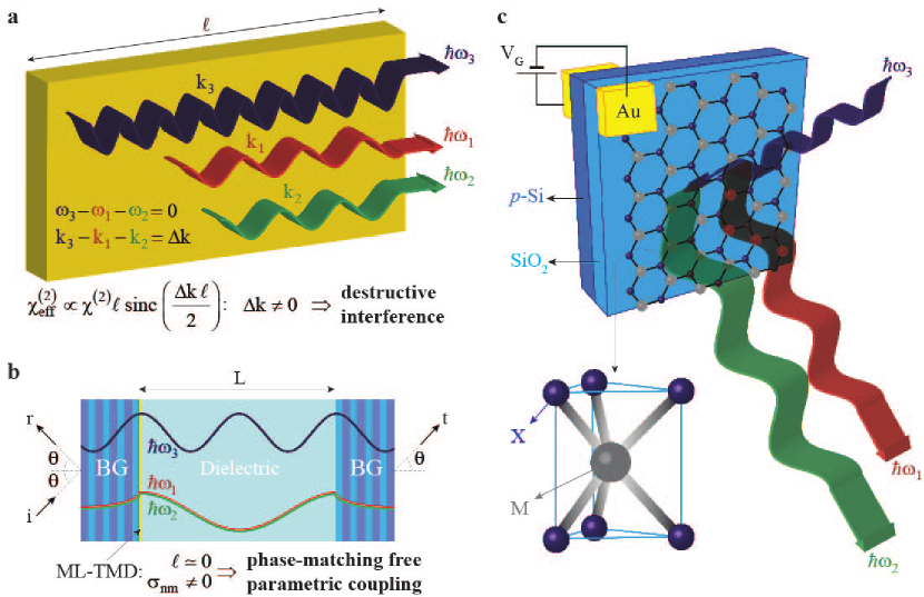
Figure 1: Phase-matching free micron-sized parametric oscillators. a. Schematic illustration of conventional three-wave parametric coupling in bulk nonlinear crystals. The effective quadratic susceptibility $\chi_{eff}^{(2)}$ is heavily affected by the mismatch $\Delta k$ among the wavevectors $k_{m}=n_{m}\omega_{m}/c$ of the pump (3), signal (1) and idler (2) waves whose destructive interference $\Delta k\neq 0$ hinders parametric coupling. b. Sketch of the ML-TMD based parametric oscillator. The cavity is assembled by two Bragg mirrors separated by a dielectric layer and the ML-TMD is placed on the left mirror. The incident (i) pump field produces both reflected (r) and transmitted (t) pump, signal and idler fields. The three-waves have negligible mutual dephasing inside the nonlinear ML-TMD (with quadratic surface conductivity $\sigma_{nm}\neq 0$) as $\ell\simeq 0$; this enables phase-matching free parametric coupling. c. Sketch of the geometry of MX₂ ML-TMDs. Fast modulation is enabled by extrinsic doping through a gate voltage with gold contacts applied between the ML-TMD and the Bragg mirror.

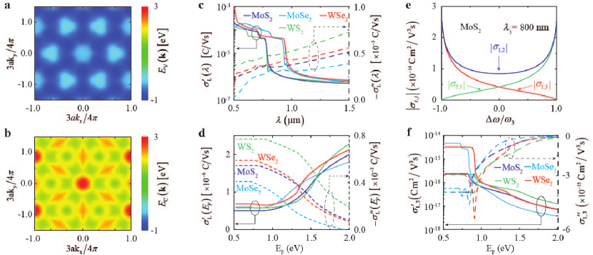
Figure 2: Electronic and optical properties of MX₂. a,b. Valence $E_{\rm V}({\bf k})$ and conduction $E_{\rm C}({\bf k})$ energy bands of MoS₂, where ${\bf k}$ is the electron wave-vector and $a=3.19\r{A}$ is the lattice parameter. c,d. Dependence of the linear surface conductivities of ML-TMDs on (c) the vacuum wavelength $\lambda$ (for intrinsic doping $E_{\rm F}=0$) and on (d) the Fermi level $E_{\rm F}$ ensuing from extrinsic doping (at $\lambda=1.6$ $\mu$m). e. PDC mixing surface conductivities of MoS₂ at $\lambda_{3}=800$ nm as a function of the angular frequency mismatch of down-converted signal and idler waves $\Delta\omega=\omega_{1}-\omega_{2}$ rescaled to the pump angular frequency $\omega_{3}$. f. Dependence of the real and imaginary parts of the PDC mixing conductivity $\sigma_{1,3}$ of MX₂ ML-TMDs on the Fermi level $E_{\rm F}$ for $\lambda_{1}=\lambda_{2}=1.6$ $\mu$m, and $\lambda_{3}=0.8$ $\mu$m.

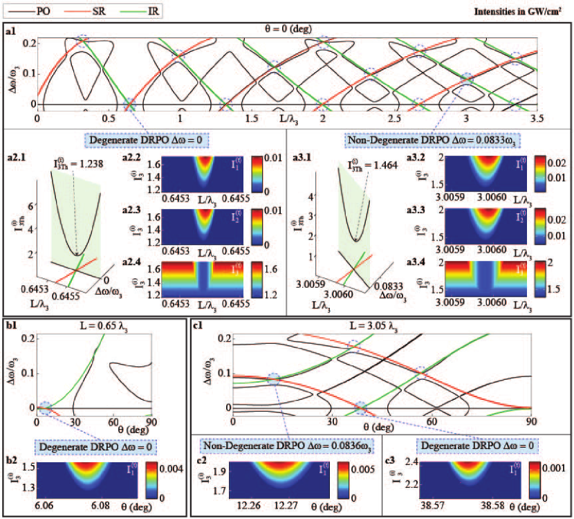
Figure 3: Parametric Oscillations. Analysis of the doubly resonant parametric oscillations (DRPOs) of a cavity (with PMMA as cavity dielectric) illuminated by a $\lambda_{3}=780$ nm pump with micron-sized Bragg Mirrors whose stop bad is centered at $1560$ nm. In subfigure a the cavity length is used as tuning parameter for normal incidence $\theta=0$ whereas in b and c the incidence angle $\theta$ is the tuning parameter for two assigned cavity lengths. a1. Identification of DRPOs as intersection among the parametric oscillation (PO) curve and the signal resonance (SR) and idler resonance (IR) curves in the ($L/\lambda_{3},\Delta\omega/\omega_{3}$) plane. a2 Intensity analysis of the degenerate ($\Delta\omega=0$) DRPO located at $L\simeq 0.645\lambda_{3}$ comprising the plots of (a2.1) the intensity threshold $I_{3Th}^{(i)}$ versus $L/\lambda_{3}$ and $\Delta\omega/\omega_{3}$ and (a2.2-4) the intensities $I_{1}^{(t)},I_{2}^{(t)},I_{3}^{(t)}$ of the transmitted signal, idler and pump fields as functions of the scaled cavity length $L/\lambda_{3}$ and the incident pump intensity $I_{3}^{(i)}$. a3 Intensity analysis of the non-degenerate ($\Delta\omega\neq 0$) DRPO located at $L\simeq 3\lambda_{3}$ (the panels are the analogous of those of a2). b1. DRPOs analysis on the ($\theta,\Delta\omega/\omega_{3}$) plane for $L$ as in a2. Note that the degenerate DRPO occurs at a small angle $\theta$. b2. Signal intensity analysis of the DRPO showing a feasible $\theta$ range. c1. DRPOs analysis on the ($\theta,\Delta\omega/\omega_{3}$) plane for $L$ as in a3 revealing a variety of DRPOs ad different angles $\theta$. c2,c3 signal intensity analysis of two DRPOs identified in c1.

Since three-wave parametric coupling is intrinsically weak, one can achieve low oscillation thresholds only by doubly or triply resonant optical cavities. In addition, parametric effects are severely hampered by the destructive interference among the three waves propagating with different wavenumbers $k_{1,2,3}$ in the dispersive nonlinear medium because the momentum mismatch $\Delta k=k_{3}-k_{2}-k_{1}$ does not generally vanish (see Fig.1a). To avoid this highly detrimental effect, the use of phase-matching (PM) strategies is imperative. The commonly-adopted birefringence-PM method Giordmaine1962 is critically sensible to the nonlinear medium orientation. Quasi-PM Vodopyanov2004 ; Canalias2007 exploits the momentum due to a manufactured long-scale periodic reversal of the sign of the nonlinear susceptibility and cannot be easily applied in miniaturized system. In semiconductors, PM is achieved by the S-shaped energy-momentum polariton dispersion in the strong coupling of excitons and photons Savvidis2000 ; Ciuti2000 , only accessible at low temperatures and large pump angles. Cavity PM Xie2011 , also denoted “relaxed” PM Clément2015 , occurs in Fabry-Perot microcavities with cavity length $\ell$ shorter than the coherence length $\pi/\Delta k$; this technique drastically reduces the effective quadratic susceptibility $\chi_{\rm eff}^{(2)}$ (see Fig.1a). Any of the above mentioned PM techniques entails a non-trivial setup design that is further constrained by the need of resonance operation.

In this manuscript, we show that emerging two-dimensional (2D) materials with high quadratic nonlinearity open unprecedented possibilities for tunable parametric micro-sources. Very remarkably, when illuminated with different visible and infrared waves, these novel 2D materials provide a negligible dispersive dephasing owing to their atomic-scale thickness (i.e $\ell\simeq 0$, see Fig.1b). Due to the lack of destructive interference, 2D materials support PDC without any need of satisfying a PM condition. Furthermore, these “phase-matching-free” devices turn out to be very versatile and compact, with the additional tunability offered by electrical gating of 2D materials, which provides ultrafast electrical-modulation functionality.

The most famous 2D material, graphene, is not the best candidate for PDC owing to the centrosymmetric structure. In principle, a static external field may break centrosymmetry and induce a $\chi_{\rm eff}^{(2)}$, but the spectrally-flat absorption of graphene is severely detrimental for PDC. Recent years have witnessed the rise of transition metal dichalcogenides (TMDs) as promising photonic 2D materials. TMDs possess several unusual optical properties dependent on the number of layers. Bulk TMDs are semiconductors with an indirect bandgap, but the optical properties of their monolayer (ML) counterpart are characterized by a direct bandgap ranging from $\sim$ 1.55 eV to $\sim$ 1.9 eV Mak2010 ; Splendiani2010 ; Wang2012 that is beneficial for several optoelectronic applications Sun2016 . In addition, ML-TMDs have broken centrosymmetry and thus undergo second-order nonlinear processes Kumar2013 ; Li2013 ; Malard2013 ; Janisch2014 ; Le2016 . Here we study PDC in micro-cavities embedding ML-TMDs; we find that the cavity design is extremely flexible if compared to standard parametric oscillators thanks to their phase-matching-free operation (see Figs.1a,1b). We demonstrate that, at conventional infrared pump intensity, parametric oscillation occurs in wavelength-sized micro-cavities with ML-TMDs. We show that the output signal and idler frequencies can be engineers thanks to the mode selectivity of doubly-resonant cavities; these frequencies are tuned by the pump incidence angle and modulated electrically by an external gate voltage.

II Results

Two hexagonal lattices of chalcogen atoms embedding a plane of metal atoms arranged at trigonal prismatic sites between the chalcogen neighbors form the structure of ML-TDMs. Wang2012 Figure 1c shows the lattice structure of MX₂ ML-TMDs (M $=$ Mo, W, and X $=$ S, Se), and Figs.2a and 2b report the valence and conduction bands of MoS₂ obtained from tight-binding calculations LWY2013 ; EPAPS . The electronic band structure of other MX₂ materials considered is qualitatively similar. The direct bandgap is about $1.5$ eV and implies transparency for infrared radiation; the linear surface conductivity has very small real part (corresponding to absorption) and higher imaginary part at infrared wavelengths. Figure 2c shows the wavelength dependence of the linear surface conductivities of MX₂. In the presence of an external pump field with angular frequency $\omega_{3}$, the ML-TMD second-order nonlinear processes lead to down-converted signal and idler waves with angular frequencies $\omega_{1}$ and $\omega_{2}$, such that $\omega_{3}=\omega_{1}+\omega_{2}$. Figure 2e illustrates the PDC mixing surface conductivities for MoS₂. Both linear and nonlinear conductivities are calculated by a perturbative expansion of the tight-binding Hamiltonian of MX₂ [see Methods and Supplementary Information (SI)]. For infrared photons with energy smaller than the bandgap, extrinsic doping by an externally applied gate voltage (see Fig.1c) modifies the optical properties and leads to an increase of absorption due to free-carrier collisions and to smaller PDC mixing conductivities. Figures 2d and 2f show the dependence of linear and nonlinear surface conductivities on the Fermi level $E_{\rm F}$. As detailed below, extrinsic doping generally leads to a decrease of PDC efficiency.

Figure 1b shows the parametric oscillator design with ML-TMDs. The cavity consists of a dielectric slab (thickness $L$) surrounded by two Bragg grating mirrors (BGs); the ML-TMD is placed on the left BG inside the cavity. The cavity is illuminated from the left by an incident (i) pump field (frequency $\omega_{3}$) and the oscillator produces both reflected (r) and transmitted (t) signal and idler fields with frequencies $\omega_{1}=(\omega_{3}+\Delta\omega)/2$ and $\omega_{2}=(\omega_{3}-\Delta\omega)/2$, where $\Delta\omega$ is the beat-note frequency of the parametric oscillation (PO).

As detailed in Methods, the cavity equations for the fields do not contain the momentum mismatch $\Delta k$. Indeed, due to their atomic thickness, ML-TMDs are not optically characterized by a refractive index but rather by a surface conductivity. Hence, the parametric coupling produced by the quadratic surface current of ML-TMDs is not hampered by dispersion and no PM condition is required accordingly. In order to observe signal and idler generation, only the PO condition is required along with the signal resonance (SR) and idler resonance (IR) conditions leading to a dramatic reduction of the intensity threshold (see Methods). Since there is no PM requirement, such requirements can be met by adjusting either the cavity length $L$ or the pump incidence angle $\theta$ as tuning parameters. For SR and IR, one needs highly reflective mirrors for both signal and idler (see Methods), as obtained by locating stop band of the micron-sized BGs at the half of the pump frequency $\omega_{3}/2$ EPAPS . Figure 3 shows the PO analysis for a cavity composed of two BGs with polymethyl methacrylate (PMMA) and MoS₂ deposited on the left mirror. The infrared pump has wavelength $\lambda_{3}=780$ nm in the spectral region where the nonlinear properties of MoS₂ are very pronounced (see Fig.2e). The BGs are tuned with their stop bands centered at $1560$ nm ($=2\lambda_{3}$) EPAPS . In Fig.3a we consider the case of normal incidence $\theta=0$ and we plot the PO (black), SR (red), and IR (green) curves in the ($L/\lambda_{3},\Delta\omega/\omega_{3}$) plane. Doubly resonant POs (DRPOs) corresponding to the intersection points of these three curves EPAPS are labeled by dashed circles. Therefore, at pump normal incidence, degenerate ($\Delta\omega=0$) and non-degenerate ($\Delta\omega\neq 0$) DRPOs exist at specific cavity lengths. Note that such oscillations also occur for sub-wavelength cavity lengths ($L<\lambda_{3}$). Each oscillation starts when the incident pump intensity $I_{3}^{(i)}$ is larger than a threshold $I_{3Th}^{(i)}$ (see Methods) EPAPS . Figures 3a2 and 3a3 show the threshold for two specific degenerate and non-denegenerate DRPOs.Panels a2.1 and a3.1 of Fig.3 report the thresholds (black curves on the shadowed vertical planes) corresponding to the PO (black) curves; one can observe that the minimum thresholds occur at SR and IR (identified by the intersection between red and green curves). The minimum intensity thresholds are of the order of GW$/$cm² and the non-degenerate DRPO threshold is greater than the degenerate DRPO one because the reflectivity of the Bragg mirror is maximum at $\Delta\omega=0$ (i.e. at half the pump frequency, as discussed above). In panels a2.2, a2.3 and a2.4 of Fig. 3 (and, seemingly, panels a3.2, a3.3 and a3.4) we report the basic DRPO features by plotting the intensities $I_{1}^{(t)},I_{2}^{(t)},I_{3}^{(t)}$ of the transmitted signal, idler and pump fields as functions of the scaled cavity length $L/\lambda_{3}$ and the incident pump intensity. Note that, in the considered example, the range of $L/\lambda_{3}$ where the oscillation actually occurs is rather narrow owing to the adopted BGs high reflectivity.

We emphasize that tuning of the PO may be realized by the pump incidence angle $\theta$, which negligibly affects the oscillation thresholds. In Fig.3b and 3c, we analyze the DRPOs by using $\theta$ as tuning parameter for a given cavity length. In particular, in Fig.3b we consider a cavity with fixed length as in Fig.3a2. The PO, SR and IR curves of Fig.3b1 intersect at a degenerate DRPO point at $\theta\simeq 6$ deg. In Fig.3b2 we plot the transmitted signal intensity $I_{1}^{(t)}$ as a function of the pump incidence angle and intensity $I_{3}^{(i)}$; one can observe that the intensity threshold is comparable to the case in Fig.3a2 and the range of angles $\theta$ where PO occurs is of the order of a hundredth of degree and experimentally feasible. We show similar results in Figs.3c1 and 3c2, where the non-degenerate DRPO of Fig.3a3 is investigated in a cavity with slightly different length, and achieved at a finite incident angle with unchanged note-beat frequency $\Delta\omega$. A more accurate analysis of Fig.3c1 also reveals that, for a given $L$, the cavity sustains multiple DRPOs (both degenerate and non-degenerate) at different incidence angles $\theta$. In Fig.3c3 we plot the transmitted intensity of a degenerate DRPO that grows with the pump intensity above the ignition threshold.

The novel PO with ML-TMDs as nonlinear media are PM-free because of the atomic size of ML-TMDs. The reported several examples of POs with MoS₂ can be also designed by other families of ML-TMDs leading to qualitatively similar results. In the Supplementary Material, we compare the calculated dependence of the pump intensity threshold as function of wavelength $\lambda_{3}$ for parametric oscillators embedding MoS₂, WS₂ and MoSe₂, WSe₂; we find that the chosen material affects the minimal threshold intensity in a given spectral range. One can optimize the choice of the material for a desired spectral content and threshold level.

A further degree of freedom offered by ML-TMDs lies in the electrical tunability through an external gate voltage, as depicted in Fig.1c. The gate voltage increases the Fermi level, and hence affects nonlinearity and absorption because of the electron-electron collision in the conduction band (see Figs.2d,f). Although electrical tunability of MX₂ has not been hitherto experimentally demonstrated, to the best of our knowledge, we emphasize that such a further degree of freedom is absent in traditional parametric oscillators. In the Supplementary Material, we report the pump intensity threshold as a function of the Fermi level of MoS₂, and we show that the threshold may increase by one order of magnitude. The external gate voltage can switch-off PO at fixed optical pump, and fast electrical modulation of the output signal and idler fields can be achieved.

III Conclusions

POs can be excited in micron-sized cavities embedding ML-TMDs as nonlinear media at conventional pump intensities in a PM-free regime. The cavity design remains inherently free of the complexity imposed by the need for PM and may result into doubly resonant PDC of signal and idler waves. The flexibility offered by such a novel oscillator design enables the engineering of selective degenerate or non-degenerate down-converted excitations by simply modifying the incident angle of the pump field. Furthermore, the electrical tunability of ML-TMDs can modulate fast output signal and idler waves by bringing POs below threshold. Based on our calculations, we envisage that novel parametric oscillators embedding ML-TMDs are a new technology for all the applications in which highly-miniaturized tunable source are relevant, including enviromental detection, security, biophyics, imaging and spectroscopy. PM-free ML-TMD microresonators may also potentially boost the realization of micrometric sources of entangled photons when pumped slightly below threshold, thus paving the way for the development of integrated quantum processors.

IV Methods

Parametric down-conversion of MX₂. We calculate the linear and PDC mixing surface conductivities of MX₂ starting from the tight-binding (TB) Hamiltonian of the electronic band structure LWY2013 . Since the properties of infrared photons with energies smaller than the bandgap are determined by small electron momenta around the K and K’ valleys, we approximate the full TB Hamiltonian as a sum of ${\bf k}\cdot{\bf p}$ Hamiltonians of first and second order $H_{0}({\bf k},\tau,s)$ EPAPS , where ${\bf k}$ is the electron wavenumber and $\tau$ and $s$ are the valley and spin indexes, respectively. We then derive the light-driven electron dynamics through the minimal coupling prescription leading to the time-dependent Hamiltonian $H_{0}\left[{\bf k}+(e/\hbar){\bf A}(t),\tau,s\right]$, where $-e$ is the electron charge, $\hbar$ is the reduced Planck constant, and ${\bf A}(t)$ is the radiation potential vector, and we obtain Bloch equations for the interband coherence and the population inversion. Finally, we solve perturbatively the Bloch equations of ML-TMDs in the weak excitation limit, obtaining the surface current density ${\bf K}(t)$ after integration over the reciprocal space

$${\bf K}(t) = {\rm Re}\left\{\sum_{j=1}^{3}\left[\hat{\sigma}^{\rm L}(\omega_{j}){\bf E}_{j}{\rm e}^{-i\omega_{j}t}\right]+\hat{\sigma}^{(1,2)}{\bf E}_{1}{\bf E}_{2}{\rm e}^{-i\omega_{3}t}+\right.$$ (1)

$$\left.+\hat{\sigma}^{(1,3)}{\bf E}_{1}^{*}{\bf E}_{3}{\rm e}^{-i\omega_{2}t}+\hat{\sigma}^{(2,3)}{\bf E}_{2}^{*}{\bf E}_{3}{\rm e}^{-i\omega_{1}t}\right\},$$

where $\hat{\sigma}^{\rm L}(\omega_{j})$ ($j=1,2,3$) and $\hat{\sigma}^{(l,m)}$ ($l,m=1,2,3$) are the linear and PDC surface conductivity tensors, respectively. Note that our approach is based on the independent-electron approximation and is fully justified only for infrared photons far from exciton resonances occurring at photon energies higher than $1.5$ eV Ugeda2014 ; Selig2016 .

Parametric oscillations. The signal, idler and pump fields, labelled with subscripts $1,2,3$ respectively, have frequencies $\omega_{n}$ satisfying $\omega_{1}+\omega_{2}=\omega_{3}$. By the Transfer Matrix approach, the full electromagnetic analysis of the cavity (see Supplementary Material) yields the equations

$$\Delta_{1}Q_{1}+\tilde{\sigma}_{23}Q_{2}^{*}Q_{3} = 0,$$

$$\Delta_{2}Q_{2}+\tilde{\sigma}_{13}Q_{1}^{*}Q_{3} = 0,$$

$$\Delta_{3}Q_{3}+\tilde{\sigma}_{12}Q_{1}Q_{2} = P_{3},$$ (2)

where $Q_{1},Q_{2},Q_{3}$ are complex amplitudes proportional to the output fields produced by the pump field which is proportional to the amplitude $P_{3}$. Here $\tilde{\sigma}_{nm}$ are scaled quadratic conductivities of the MX₂ ML-TMD and

$$\Delta_{n} = \tilde{\sigma}_{n}-\frac{c}{\omega_{n}}q_{n}\left({\frac{{r_{n}^{\left(R\right)}-1}}{{r_{n}^{\left(R\right)}+1}}+\frac{{r_{n}^{\left(R\right)}e^{iq_{n}L}-e^{-iq_{n}L}}}{{r_{n}^{\left(R\right)}e^{iq_{n}L}+e^{-iq_{n}L}}}}\right).$$ (3)

are parameters characterizing the linear cavity where $\tilde{\sigma}_{n}$ are scaled linear surface conductivities, $q_{n}=\frac{\omega_{n}}{c}\sqrt{\varepsilon\left({\omega_{n}}\right)-\sin^{2}\theta}$ are the longitudinal wavenumbers inside the dielectric slab, $\epsilon(\omega)$ is the relative permittivity of the dielectric slab, $\theta$ is the pump incidence angle whereas $r_{n}^{\left(R\right)}$ are the complex reflectivities for right illumination of the left Bragg mirror (with vacuum and the dielectric slab on its left and right sides, respectively). It is worth stressing that the phase-mismatch $\Delta k=k_{3}-k_{1}-k_{2}$ does not appear in the basic cavity equations (IV). Hence parametric coupling is here not affected by the fields destructive interference and the phase-matching constraint is strictly avoided. Paramateric oscillations (POs) are solutions of Eqs.(IV) with $Q_{1}\neq 0$ and $Q_{2}\neq 0$ and in this case the compatibility of the first two equations yields (see Supplementary Material)

$$\left|{P_{3}}\right|^{2}\geq\frac{{\Delta_{1}\Delta_{2}^{*}}}{{\tilde{\sigma}_{23}\tilde{\sigma}_{13}^{*}}}\left|{\Delta_{3}}\right|^{2},$$ (4)

which is the leading PO condition. As the right hand side of Eq. (39) is generally a complex number, for the PO we have the condition

$${\rm arg}\left(\frac{\Delta_{1}}{\tilde{\sigma}_{23}}\right)={\rm arg}\left(\frac{\Delta_{2}}{\tilde{\sigma}_{13}}\right).$$ (5)

Eq. (5) can be physically interpreted as a locking of the phase difference ${\arg Q_{1}}-{\arg Q_{2}^{*}}$ allowing the signal and idler to oscillate. Once Eq.(5) is satisfied, Eq.(39) provides the pump threshold for the onset of PO. Due to the absolute smallness of the nonlinear surface conductivities, in order to have a feasible threshold, the cavity parameters $|\Delta_{n}|$ must be minimized. This can be obtained by choosing the doubly resonant condition for signal and idler corresponding to the minima of $|\Delta_{1}|$ and $|\Delta_{2}|$, respectively. In order for this minima to be very small, we need that $|r_{1}^{\left(R\right)}|$ and $|r_{2}^{\left(R\right)}|$ are very close to one. One can satisfy such a constraint by a suitable Bragg mirror design to have the stop-band centered at the half of the pump frequency $\omega_{3}/2$ since, in this case, signal and idler fields experience large mirror reflectance.

Here we provide additional information on technical aspects of the theoretical methods used to model parametric down-conversion and the resulting phase-matching free resonant oscillations within the micro-cavities described in the main paper.

Appendix A Parametric down-conversion of MX₂

We calculate the linear and parametric down-conversion (PDC) mixing surface conductivities of monolayer (ML) transition metal dichalcogenides (TMDs) MX₂ (M $=$ Mo, S, and X $=$ S, Se) starting from a tight-binding (TB) description of the electronic band structure of these materials LWY2013 and studying the light-driven electron dynamics by means of Bloch equations for the valence and conduction bands. Note that our approach is based on the independent-electron approximation and is fully justified at the frequencies considered in the main paper since they are far from exciton resonances happening at photon energies of $\simeq 1.5$ eV or higher UBS2014 ; CCB2016 . In addition, for the infrared photon energies considered, the relevant valence and conduction band regions affecting the infrared response are the ones closer to the band gap around the K and K’ band edges, for which the full TB Hamiltonian can be approximated by a two-band ${\bf k}\cdot{\bf p}$ Hamiltonian ${\cal H}_{0}({\bf k},\tau,s)={\cal H}_{1}({\bf k},\tau,s)+{\cal H}_{2}({\bf k},\tau)$ LWY2013 , where

$${\cal H}_{1}({\bf k},\tau,s)=\left[\begin{array}[]{cc}\Delta/2&t_{0}a(\tau k_{x}-ik_{y})\\ t_{0}a(\tau k_{x}+ik_{y})&\tau s\Lambda-\Delta/2\end{array}\right],$$ (8)

$${\cal H}_{2}({\bf k},\tau,s)=\left[\begin{array}[]{cc}\gamma_{1}a^{2}k^{2}&\gamma_{3}a^{2}(\tau k_{x}+ik_{y})^{2}\\ \gamma_{3}a^{2}(\tau k_{x}-ik_{y})^{2}&\gamma_{2}a^{2}k^{2}\end{array}\right],$$ (11)

and $\tau,s=\pm 1$ label non-degenerate valleys and spins, while ${\bf k}=(k_{x}~{}k_{y})$ indicates the electron wave-vector.

Table S1: Fitted constants of the the two-band ${\bf k}\cdot{\bf p}$ Hamiltonian ${\cal H}_{0}({\bf k},\tau,s)$.

Constants	MoS2	MoSe2	WS2	WSe2
$a$ (Å)	$3.190$	$3.326$	$3.191$	$3.325$
$\Delta$ (eV)	$1.658$	$1.429$	$1.806$	$1.541$
$t_{0}$ (eV)	$0.933$	$0.768$	$1.196$	$1.016$
$\Lambda$ (eV)	$0.073$	$0.091$	$0.211$	$0.228$
$\gamma_{1}$ (eV)	$0.351$	$0.291$	$0.443$	$0.404$
$\gamma_{2}$ (eV)	$-0.198$	$-0.191$	$-0.211$	$-0.216$
$\gamma_{3}$ (eV)	$-0.143$	$-0.099$	$-0.199$	$-0.150$

The physical parameters of ${\cal H}_{0}({\bf k},\tau,s)$ are obtained by fitting the ${\bf k}\cdot{\bf p}$ valence and conduction energy bands with the ones obtained from first-principles GW simulations LWY2013 accounting for both non-degenerate valleys and spin-orbit coupling, and are listed in Table S1. We calculate the linear and PDC mixing conductivities of ML-TMDs by introducing the time-dependent Hamiltonian ${\cal H}_{0}(\mbox{\boldmath${\kappa}$}(t),\tau,s)$, where we have replaced the electron wave-vector with the minimum coupling prescription for the electron quasi-momentum $\hbar\mbox{\boldmath${\kappa}$}(t)=\hbar{\bf k}+e{\bf A}(t)$, where $e$ is the electron charge and ${\bf A}(t)$ is the electromagnetic potential vector accounting for pump, signal, and idler waves. With this prescription, we define unperturbed and interacting Hamiltonians ${\cal H}_{0}({\bf k},\tau,s)$ and ${\cal H}_{\rm I}({\bf k},\tau,s,t)$, respectively, and write the total Hamiltonian as ${\cal H}_{\rm T}({\bf k},\tau,s,t)={\cal H}_{0}[\mbox{\boldmath${\kappa}$}(t),\tau,s]={\cal H}_{0}({\bf k},\tau,s)+{\cal H}_{\rm I}({\bf k},\tau,s,t)$, where

$${\cal H}_{\rm I}({\bf k},\tau,s,t) = \frac{e}{\hbar}[D_{x}A_{x}(t)+D_{y}A_{y}(t)]+\frac{e^{2}}{\hbar^{2}}[D_{xx}A_{x}^{2}(t)+D_{xy}A_{x}(t)A_{y}(t)+D_{yy}A_{y}^{2}(t)],$$ (13)

and the interaction operators are explicitly given by

$$D_{x}=t_{0}a\tau\left[|\psi_{\rm V}\rangle\langle\psi_{\rm C}|+|\psi_{\rm C}\rangle\langle\psi_{\rm V}|\right],$$

$$D_{y}=it_{0}a\left[|\psi_{\rm V}\rangle\langle\psi_{\rm C}|-|\psi_{\rm C}\rangle\langle\psi_{\rm V}|\right],$$

$$D_{xx}=\gamma_{1}a^{2}|\psi_{\rm C}\rangle\langle\psi_{\rm C}|+\gamma_{2}a^{2}|\psi_{\rm V}\rangle\langle\psi_{\rm V}|+\gamma_{3}a^{2}\left[|\psi_{\rm V}\rangle\langle\psi_{\rm C}|+|\psi_{\rm C}\rangle\langle\psi_{\rm V}|\right],$$

$$D_{yy}=\gamma_{1}a^{2}|\psi_{\rm C}\rangle\langle\psi_{\rm C}|+\gamma_{2}a^{2}|\psi_{\rm V}\rangle\langle\psi_{\rm V}|-\gamma_{3}a^{2}\left[|\psi_{\rm V}\rangle\langle\psi_{\rm C}|+|\psi_{\rm C}\rangle\langle\psi_{\rm V}|\right],$$

$$D_{xy}=2i\gamma_{3}a^{2}\tau\left[|\psi_{\rm C}\rangle\langle\psi_{\rm V}|-|\psi_{\rm V}\rangle\langle\psi_{\rm C}|\right].$$

In the expressions above we use the Dirac notation for the conduction $|\psi_{\rm C}\rangle$ and valence $|\psi_{\rm V}\rangle$ band eigenstates, and we approximate the matrix elements by their values at the band edges (${\bf k}=0$). Inserting the Ansatz $|\psi\rangle=c_{-}|\psi_{\rm V}\rangle+c_{+}|\psi_{\rm C}\rangle$ in the time-dependent Schrödinger equation $i\hbar\partial_{t}|\psi\rangle={\cal H}_{\rm T}|\psi\rangle$, and defining the inversion population $n_{\bf k}=|c_{+}|^{2}-|c_{-}|^{2}$ and the interband coherence $\rho_{\bf k}=c_{+}c_{-}^{*}$, one gets

$$\dot{\rho}_{\bf k} = -\frac{i}{\hbar}(E_{\rm C}-E_{\rm V})\rho_{\bf k}-\gamma\rho_{\bf k}+\frac{ie}{\hbar^{2}}n_{\bf k}\left\{D_{x}^{\rm CV}A_{x}(t)+D_{y}^{\rm CV}A_{y}(t)+\frac{e}{\hbar}[D_{xx}^{\rm CV}A_{x}^{2}(t)+D_{xy}^{\rm CV}A_{x}(t)A_{y}(t)+D_{yy}^{\rm CV}A_{y}^{2}(t)]\right\}+$$

$$+\frac{ie^{2}}{\hbar^{3}}\left[(D_{xx}^{\rm VV}-D_{xx}^{\rm CC})A_{x}^{2}(t)+(D_{yy}^{\rm VV}-D_{yy}^{\rm CC})A_{y}^{2}(t)\right]\rho_{\bf k},$$

$$\dot{n}_{\bf k} = -\frac{4e}{\hbar^{2}}{\rm Im}\left\{\rho_{\bf k}\left[D_{x}^{\rm VC}A_{x}(t)+D_{y}^{\rm VC}A_{y}(t)+\frac{e}{\hbar}[D_{xx}^{\rm VC}A_{x}^{2}(t)+D_{xy}^{\rm VC}A_{x}(t)A_{y}(t)+D_{yy}^{\rm VC}A_{y}^{2}(t)]\right]\right\},$$ (15)

where $E_{\rm C}({\bf k})$ and $E_{\rm V}({\bf k})$ are the conduction and valence energy bands of the unperturbed Hamiltonian ${\cal H}_{0}$, $D^{\rm CV}_{j}=\langle\psi_{\rm C}|D_{j}|\psi_{\rm V}\rangle$ are the interaction matrix elements, and we have introduced a phenomenological relaxation rate $\gamma=10$ ps^-1 accounting for coherence dephasing YYC2014 . In order to obtain the PDC surface conductivities, we consider a coherent superposition of three monochromatic fields ${\bf E}(t)={\rm Re}\left\{{\bf E}_{1}{\rm e}^{-i\omega_{1}t}+{\bf E}_{2}{\rm e}^{-i\omega_{2}t}+{\bf E}_{3}{\rm e}^{-i\omega_{3}t}\right\}$ with amplitudes ${\bf E}_{1}$, ${\bf E}_{2}$, and ${\bf E}_{3}$, and with angular frequencies $\omega_{1}$, $\omega_{2}$, and $\omega_{3}$, respectively. In our notation, the field ${\bf E}_{3}$ indicates the external pump field, while ${\bf E}_{1}$, ${\bf E}_{2}$ label the down-converted signal and idler fields, respectively. The down-converted angular frequencies $\omega_{1}$ and $\omega_{2}$ are not independent, but are such that $\omega_{1}+\omega_{2}=\omega_{3}$ owing to energy conservation. The electromagnetic potential vector related to the coherent superposition of pump, signal, and idler waves is thus given by

$${\bf A}(t)={\rm Re}\left\{({\bf E}_{1}/i\omega_{1}){\rm e}^{-i\omega_{1}t}+({\bf E}_{2}/i\omega_{2}){\rm e}^{-i\omega_{2}t}+({\bf E}_{3}/i\omega_{3}){\rm e}^{-i\omega_{3}t}\right\}.$$ (16)

We then solve perturbatively the equations above in the vanishing temperature $T\rightarrow 0$ and weak excitation limits such that $n_{\bf k}\approx-\Theta\left[E_{\rm C}({\bf k})-E_{\rm F}\right]$, where $\Theta(x)$ indicates the Heaviside step function and $E_{\rm F}$ is the Fermi energy. Taking the Ansatz $\rho_{\bf k}=\sum_{j=\pm 1,\pm 2,\pm 3}\rho_{|j|}^{(j/|j|)}{\rm e}^{i(j/|j|)\omega_{|j|}t}$ and disregarding generation of higher harmonics we obtain analytical expressions for the coefficients $\rho_{|j|}^{(j/|j|)}$, finding that the macroscopic surface current density given by

$${\bf K}(t) = -\frac{e}{4\pi^{2}\hbar}\sum_{\tau,s=-1,1}\int_{-\infty}^{+\infty}dk_{x}\int_{-\infty}^{+\infty}dk_{y}\left[\langle\psi(t)|\nabla_{\bf k}{\cal H}_{\rm T}(t)|\psi(t)\rangle-\langle\psi_{\rm V}|\nabla_{\bf k}{\cal H}_{\rm T}(t)|\psi_{\rm V}\rangle\right]=$$

$$= -\frac{e}{2\pi^{2}\hbar}\sum_{\tau,s=-1,1}\int_{-\infty}^{+\infty}dk_{x}\int_{-\infty}^{+\infty}dk_{y}{\rm Re}\left\{\rho_{\bf k}(t)\left[\nabla_{\bf k}{\cal H}_{0}^{\rm VC}+\nabla_{\bf k}D_{x}^{\rm VC}\frac{e}{\hbar}A_{x}(t)+\nabla_{\bf k}D_{y}^{\rm VC}\frac{e}{\hbar}A_{y}(t)+\right.\right.$$

$$\left.\left.+\nabla_{\bf k}D_{xx}^{\rm VC}\frac{e^{2}}{\hbar^{2}}A_{x}^{2}(t)+\nabla_{\bf k}D_{xy}^{\rm VC}\frac{e^{2}}{\hbar^{2}}A_{x}(t)A_{y}(t)+\nabla_{\bf k}D_{yy}^{\rm VC}\frac{e^{2}}{\hbar^{2}}A_{y}^{2}(t)\right]+\right.$$

$$\left.+\Theta\left[E_{\rm F}-E_{\rm C}({\bf k})\right]\left[D_{xx}^{\rm CC}\frac{e}{\hbar}A_{x}(t)+D_{yy}^{\rm CC}\frac{e}{\hbar}A_{y}(t)\right]\right\},$$

can be recast into

$${\bf K}(t)={\rm Re}\left\{\sum_{j=1}^{3}\left[\hat{\sigma}^{\rm L}(\omega_{j}){\bf E}_{j}{\rm e}^{-i\omega_{j}t}\right]+\hat{\sigma}^{(1,2)}{\bf E}_{1}{\bf E}_{2}{\rm e}^{-i\omega_{3}t}+\hat{\sigma}^{(1,3)}{\bf E}_{1}^{*}{\bf E}_{3}{\rm e}^{-i\omega_{2}t}+\hat{\sigma}^{(2,3)}{\bf E}_{2}^{*}{\bf E}_{3}{\rm e}^{-i\omega_{1}t}\right\},$$ (18)

where $\hat{\sigma}^{\rm L}(\omega_{j})$ ($j=1,2,3$) and $\hat{\sigma}^{(l,m)}$ ($l,m=1,2,3$) are the linear and PDC surface conductivity tensors, respectively, and we have neglected again generation of higher harmonics. Since centrosymmetry is broken along the $y$-direction in the notation used, the relevant components of the surface conductivity tensors for PDC are the ones such that pump, signal, and idler fields are polarized along the $y$-direction, for which

$$\sigma^{\rm L}_{yy}(\omega)=\frac{ie^{2}D_{yy}^{\rm CC}}{2\pi^{2}\hbar^{2}(\omega+i\gamma)}\sum_{\tau,s=\pm 1}\int_{-\infty}^{+\infty}dk_{x}\int_{-\infty}^{+\infty}dk_{y}\Theta\left[E_{\rm F}-E_{\rm C}({\bf k})\right]+$$ (19)

$$+\frac{e^{2}}{4i\pi^{2}\hbar^{2}\omega}\sum_{\tau,s=\pm 1}\int_{-\infty}^{+\infty}dk_{x}\int_{-\infty}^{+\infty}dk_{y}\Theta\left[E_{\rm C}({\bf k})-E_{\rm F}\right]\left\{\frac{|D_{y}^{\rm CV}|^{2}}{[(E_{\rm C}-E_{\rm V})-\hbar(\omega+i\gamma)]}+\frac{|D_{y}^{\rm CV}|^{2}}{[(E_{\rm C}-E_{\rm V})+\hbar(\omega+i\gamma)]}\right\},$$

$$\sigma^{\rm(1,2)}_{yyy}(\omega_{1},\omega_{2},\omega_{3})=\frac{-e^{3}}{4\pi^{2}\hbar^{3}\omega_{1}\omega_{2}}\sum_{\tau,s=\pm 1}\sum_{j=1}^{3}\int_{-\infty}^{+\infty}dk_{x}\int_{-\infty}^{+\infty}dk_{y}\Theta\left[E_{\rm C}({\bf k})-E_{\rm F}\right]\left\{\frac{D_{y}^{\rm CV}D_{yy}^{\rm VC}}{[(E_{\rm C}-E_{\rm V})-\hbar(\omega_{j}+i\gamma)]}+\right.$$

$$\left.+\frac{D_{y}^{\rm VC}D_{yy}^{\rm CV}}{[(E_{\rm C}-E_{\rm V})+\hbar(\omega_{j}+i\gamma)]}\right\},$$

$$\sigma^{\rm(1,3)}_{yyy}(\omega_{1},\omega_{2},\omega_{3})=\frac{e^{3}}{4\pi^{2}\hbar^{3}\omega_{1}\omega_{3}}\sum_{\tau,s=\pm 1}\int_{-\infty}^{+\infty}dk_{x}\int_{-\infty}^{+\infty}dk_{y}\Theta\left[E_{\rm C}({\bf k})-E_{\rm F}\right]\left\{\frac{D_{y}^{\rm CV}D_{yy}^{\rm VC}}{[(E_{\rm C}-E_{\rm V})+\hbar(\omega_{1}-i\gamma)]}+\right.$$ (20)

$$\left.+\frac{D_{y}^{\rm VC}D_{yy}^{\rm CV}}{[(E_{\rm C}-E_{\rm V})-\hbar(\omega_{1}-i\gamma)]}+\frac{D_{y}^{\rm CV}D_{yy}^{\rm VC}}{[(E_{\rm C}-E_{\rm V})+\hbar(\omega_{2}+i\gamma)]}+\frac{D_{y}^{\rm VC}D_{yy}^{\rm CV}}{[(E_{\rm C}-E_{\rm V})-\hbar(\omega_{2}+i\gamma)]}+\right.$$

$$\left.+\frac{D_{y}^{\rm CV}D_{yy}^{\rm VC}}{[(E_{\rm C}-E_{\rm V})-\hbar(\omega_{3}+i\gamma)]}+\frac{D_{y}^{\rm VC}D_{yy}^{\rm CV}}{[(E_{\rm C}-E_{\rm V})+\hbar(\omega_{3}+i\gamma)]}\right\},$$

$$\sigma^{\rm(2,3)}_{yyy}(\omega_{1},\omega_{2},\omega_{3})=\frac{e^{3}}{4\pi^{2}\hbar^{3}\omega_{2}\omega_{3}}\sum_{\tau,s=\pm 1}\int_{-\infty}^{+\infty}dk_{x}\int_{-\infty}^{+\infty}dk_{y}\Theta\left[E_{\rm C}({\bf k})-E_{\rm F}\right]\left\{\frac{D_{y}^{\rm CV}D_{yy}^{\rm VC}}{[(E_{\rm C}-E_{\rm V})+\hbar(\omega_{1}+i\gamma)]}+\right.$$ (21)

$$\left.+\frac{D_{y}^{\rm VC}D_{yy}^{\rm CV}}{[(E_{\rm C}-E_{\rm V})-\hbar(\omega_{1}+i\gamma)]}+\frac{D_{y}^{\rm CV}D_{yy}^{\rm VC}}{[(E_{\rm C}-E_{\rm V})+\hbar(\omega_{2}-i\gamma)]}+\frac{D_{y}^{\rm VC}D_{yy}^{\rm CV}}{[(E_{\rm C}-E_{\rm V})-\hbar(\omega_{2}-i\gamma)]}+\frac{D_{y}^{\rm CV}D_{yy}^{\rm VC}}{[(E_{\rm C}-E_{\rm V})-\hbar(\omega_{3}+i\gamma)]}+\right.$$

$$\left.+\frac{D_{y}^{\rm VC}D_{yy}^{\rm CV}}{[(E_{\rm C}-E_{\rm V})+\hbar(\omega_{3}+i\gamma)]}\right\}.$$

Data reported in the main paper are obtained through the expressions above. In what follows, for convenience we will assume the simplified notation $\sigma_{n}=\sigma^{\rm L}_{yy}(\omega_{n})$ and $\sigma_{nm}=\sigma^{(n,m)}_{yyy}(\omega_{1},\omega_{2},\omega_{3})$ since the pump, signal, and idler electric fields are polarized in the $y$-direction for maximizing PDC within the micro-cavity.

Appendix B Equations for the output fields

In Fig.4 we sketch the geometry of the parametric oscillator (PO) considered in our calculations. A dielectric (PMMA) slab of thickness $L$ with a MX₂ monolayer lying on its left side (at $z=0$) is placed between two Bragg mirrors of thickness $d$ (for convenience we choose the right mirror to be the reflected $z\rightarrow-z$ copy of the left one). The left side of the cavity is illuminated with an incident $(i)$ pump field which is a monochromatic Transverse Electric (TE) plane wave of frequency $\omega_{3}$ with incidence angle $\theta$. In addition to the reflected $(r)$ and transmitted $(t)$ pump fields, due to PDC, the cavity also produces $(r)$ and $(t)$ TE plane waves at the frequencies $\omega_{1}$ (signal) and $\omega_{2}$ (idler) such that $\omega_{3}=\omega_{1}+\omega_{2}$. It is convenient to set

$$\omega_{1} = \frac{1}{2}\left(\omega_{3}+\Delta\omega\right),$$

$$\omega_{2} = \frac{1}{2}\left(\omega_{3}-\Delta\omega\right),$$ (22)

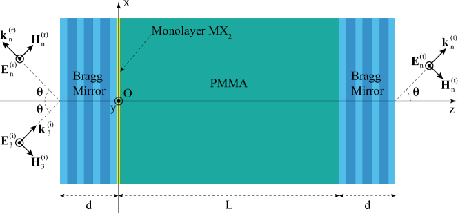
Figure 4: Parametric oscillator geometry.

since the note-beat frequency $\Delta\omega=\omega_{1}-\omega_{2}$ is sufficient to label the signal and idler frequencies produced by a pump field of frequency $\omega_{3}$. Conservation of transverse momentum of the three fields implies that the their complex amplitudes ($\sim e^{-i\omega_{n}t}$, $n=1,2,3$) are

$${\bf{E}}_{n} = e^{i\frac{\omega_{n}}{c}x\sin\theta}\left[{A_{ny}\left(z\right){\bf{\hat{e}}}_{y}}\right],$$

$${\bf{H}}_{n} = e^{i\frac{\omega_{n}}{c}x\sin\theta}\sqrt{\frac{{\varepsilon_{0}}}{{\mu_{0}}}}\left[{A_{nx}\left(z\right){\bf{\hat{e}}}_{x}+A_{ny}\left(z\right)\sin\theta{\bf{\hat{e}}}_{z}}\right].$$ (23)

Accordingly the three two-component column vectors $\left(A_{nx}(z)\>A_{ny}(z)\right)^{T}$ fully describe the field and in vacuum, i.e. outside the cavity, they are

$$\begin{cases}\begin{pmatrix}{A_{nx}}\\ {A_{ny}}\\ \end{pmatrix}=E_{n}^{\left(i\right)}\begin{pmatrix}{-\cos\theta}\\ 1\\ \end{pmatrix}e^{i\frac{\omega_{n}}{c}\left({z+d}\right)\cos\theta}+E_{n}^{\left(r\right)}\begin{pmatrix}{\cos\theta}\\ 1\\ \end{pmatrix}e^{-i\frac{\omega_{n}}{c}\left({z+d}\right)\cos\theta},&z<-d,\\ \begin{pmatrix}{A_{nx}}\\ {A_{ny}}\\ \end{pmatrix}=E_{n}^{\left(t\right)}\begin{pmatrix}{-\cos\theta}\\ 1\\ \end{pmatrix}e^{i\frac{\omega_{n}}{c}\left({z-L-d}\right)\cos\theta},&z>L+d,\end{cases}$$ (24)

where $E_{n}^{\left(i\right)}$, $E_{n}^{\left(r\right)}$ and $E_{n}^{\left(t\right)}$ are field amplitudes with $E_{1}^{\left(i\right)}=E_{2}^{\left(i\right)}=0$. Resorting to the transfer matrix approach, the fields at the left ($z=0^{-}$) and right ($z=0^{+}$) sides of the MX₂ monolayer are

$$\begin{pmatrix}{A_{nx}}\\ {A_{ny}}\\ \end{pmatrix}_{z=0^{-}} = F_{n}\begin{pmatrix}{A_{nx}}\\ {A_{ny}}\\ \end{pmatrix}_{z=-d},$$

$$\begin{pmatrix}{A_{nx}}\\ {A_{ny}}\\ \end{pmatrix}_{z=0^{+}} = B_{n}B^{\prime}_{n}\begin{pmatrix}{A_{nx}}\\ {A_{ny}}\\ \end{pmatrix}_{z=L+d},$$ (25)

where $F_{n}$, $B_{n}$ and $B^{\prime}_{n}$ are the transfer matrix describing the forward, backward and backward propagations through the left Bragg mirror, the dielectric slab and the right Bragg mirror, respectively. The transfer matrix $F_{n}$ of the left Bragg mirror is the (ordered) product of the transfer matrices of the slabs composing the mirror. For later convenience it is useful to represent this matrix as Kavok

$$F_{n} = \begin{pmatrix}{\frac{{cq_{n}}}{{\omega_{n}\cos\theta}}\left[{\frac{{t_{n}^{\left(L\right)}t_{n}^{\left(R\right)}+\left({1+r_{n}^{\left(L\right)}}\right)\left({1-r_{n}^{\left(R\right)}}\right)}}{{2t_{n}^{\left(R\right)}}}}\right]}&{\frac{{cq_{n}}}{{\omega_{n}}}\left[{\frac{{-t_{n}^{\left(L\right)}t_{n}^{\left(R\right)}+\left({1-r_{n}^{\left(L\right)}}\right)\left({1-r_{n}^{\left(R\right)}}\right)}}{{2t_{n}^{\left(R\right)}}}}\right]}\\ {\frac{1}{{\cos\theta}}\left[{\frac{{-t_{n}^{\left(R\right)}t_{n}^{\left(L\right)}+\left({1+r_{n}^{\left(L\right)}}\right)\left({1+r_{n}^{\left(R\right)}}\right)}}{{2t_{n}^{\left(R\right)}}}}\right]}&{\left[{\frac{{t_{n}^{\left(L\right)}t_{n}^{\left(R\right)}+\left({1-r_{n}^{\left(R\right)}}\right)\left({1+r_{n}^{\left(R\right)}}\right)}}{{2t_{n}^{\left(R\right)}}}}\right]}\\ \end{pmatrix},$$

where $q_{n}=\frac{\omega_{n}}{c}\sqrt{\varepsilon\left({\omega_{n}}\right)-\sin^{2}\theta}$ are the longitudinal wavenumbers inside the dielectric slab, $\epsilon(\omega)$ is the relative permittivity of the dielectric slab whereas $r_{n}^{\left(L\right)},t_{n}^{\left(L\right)},r_{n}^{\left(R\right)},t_{n}^{\left(R\right)}$ are the complex reflectivities $r$ and transmittivities $t$ for left $(L)$ and right $(R)$ illumination of the left Bragg mirror (with vacuum and the dielectric on its left and right sides, respectively). The other relevant transfer matrices are Kavok

$$B_{n} = \begin{pmatrix}{\cos\left({q_{n}L}\right)}&{i\frac{{cq_{n}}}{{\omega_{n}}}\sin\left({q_{n}L}\right)}\\ {i{{\frac{\omega_{n}}{cq_{n}}}}\sin\left({q_{n}L}\right)}&{\cos\left({q_{n}L}\right)}\\ \end{pmatrix},$$

$$B^{\prime}_{n} = \begin{pmatrix}1&0\\ 0&{-1}\\ \end{pmatrix}F_{n}\begin{pmatrix}1&0\\ 0&{-1}\\ \end{pmatrix},$$ (27)

where the last of Eqs. (B) is a consequence of the fact that the right Bragg mirror is the reflected image of the left one. Using Eqs. (24), Eqs. (B) yield

$$\begin{pmatrix}{A_{nx}}\\ {A_{ny}}\\ \end{pmatrix}_{z=0^{-}} = \begin{pmatrix}{V_{nx}^{\left(i\right)}}\\ {V_{ny}^{\left(i\right)}}\\ \end{pmatrix}E_{n}^{\left(i\right)}+\begin{pmatrix}{V_{nx}^{\left(r\right)}}\\ {V_{ny}^{\left(r\right)}}\\ \end{pmatrix}E_{n}^{\left(r\right)},$$

$$\begin{pmatrix}{A_{nx}}\\ {A_{ny}}\\ \end{pmatrix}_{z=0^{+}} = \begin{pmatrix}{V_{nx}^{\left(t\right)}}\\ {V_{ny}^{\left(t\right)}}\\ \end{pmatrix}E_{n}^{\left(t\right)},$$ (28)

where

$$\begin{pmatrix}{V_{nx}^{\left(i\right)}}\\ {V_{ny}^{\left(i\right)}}\\ \end{pmatrix} = \frac{1}{{t_{n}^{\left(R\right)}}}\begin{pmatrix}{\frac{{cq_{n}}}{\omega_{n}}\left[{-t_{n}^{\left(L\right)}t_{n}^{\left(R\right)}+r_{n}^{\left(L\right)}\left({r_{n}^{\left(R\right)}-1}\right)}\right]}\\ {t_{n}^{\left(L\right)}t_{n}^{\left(R\right)}-r_{n}^{\left(L\right)}\left({r_{n}^{\left(R\right)}+1}\right)}\\ \end{pmatrix},$$

$$\begin{pmatrix}{V_{nx}^{\left(r\right)}}\\ {V_{ny}^{\left(r\right)}}\\ \end{pmatrix} = \frac{1}{{t_{n}^{\left(R\right)}}}\begin{pmatrix}{-\frac{{cq_{n}}}{{\omega_{n}}}\left({r_{n}^{\left(R\right)}-1}\right)}\\ {r_{n}^{\left(R\right)}+1}\\ \end{pmatrix},$$

$$\begin{pmatrix}{V_{nx}^{\left(t\right)}}\\ {V_{ny}^{\left(t\right)}}\\ \end{pmatrix} = \frac{1}{{t_{n}^{\left(R\right)}}}\begin{pmatrix}{\frac{{cq_{n}}}{\omega_{n}}\left({r_{n}^{\left(R\right)}e^{iq_{n}L}-e^{-iq_{n}L}}\right)}\\ {\left({r_{n}^{\left(R\right)}e^{iq_{n}L}+e^{-iq_{n}L}}\right)}\end{pmatrix}.$$ (29)

The monolayer of MX₂ in the presence of the above TE electromagnetic field hosts a surface current whose harmonic complex amplitudes are ${\bf K}_{n}=K_{n}\hat{\bf e}_{y}$ where

$$K_{1} = \left[\sigma_{1}E_{1y}+\sigma_{23}E_{2y}^{*}E_{3y}\right]_{z=0},$$

$$K_{2} = \left[\sigma_{2}E_{2y}+\sigma_{13}E_{1y}^{*}E_{3y}\right]_{z=0},$$

$$K_{3} = \left[\sigma_{3}E_{3y}+\sigma_{12}E_{1y}E_{2y}\right]_{z=0},$$ (30)

showing both a linear and a quadratic response to the electric field. The effect of such surface current on the field is provided by the electromagnetic boundary conditions at $z=0$, namely ${\bf{\hat{e}}}_{z}\times\left\{{\left[{{\bf{E}}_{n}}\right]_{z=0^{+}}-\left[{{\bf{E}}_{n}}\right]_{z=0^{-}}}\right\}={\bf{0}}$ and ${\bf{\hat{e}}}_{z}\times\left\{{\left[{{\bf{H}}_{n}}\right]_{z=0^{+}}-\left[{{\bf{H}}_{n}}\right]_{z=0^{-}}}\right\}={\bf{K}}_{n}$ which, using Eqs. (B), can be casted within the two-component column vector description as

$$\begin{pmatrix}{A_{1x}}\\ {A_{1y}}\\ \end{pmatrix}_{z=0^{+}}-\begin{pmatrix}{A_{1x}}\\ {A_{1y}}\\ \end{pmatrix}_{z=0^{-}}=\begin{pmatrix}{\tilde{\sigma}_{1}A_{1y}+\tilde{\sigma}_{23}A_{2y}^{*}A_{3y}}\\ 0\\ \end{pmatrix}_{z=0^{+}},$$

$$\begin{pmatrix}{A_{2x}}\\ {A_{2y}}\\ \end{pmatrix}_{z=0^{+}}-\begin{pmatrix}{A_{2x}}\\ {A_{2y}}\\ \end{pmatrix}_{z=0^{-}}=\begin{pmatrix}{\tilde{\sigma}_{2}A_{2y}+\tilde{\sigma}_{13}A_{1y}^{*}A_{3y}}\\ 0\\ \end{pmatrix}_{z=0^{+}},$$

$$\begin{pmatrix}{A_{3x}}\\ {A_{3y}}\\ \end{pmatrix}_{z=0^{+}}-\begin{pmatrix}{A_{3x}}\\ {A_{3y}}\\ \end{pmatrix}_{z=0^{-}}=\begin{pmatrix}{\tilde{\sigma}_{3}A_{3y}+\tilde{\sigma}_{12}A_{1y}A_{2y}}\\ 0\\ \end{pmatrix}_{z=0^{+}},$$ (31)

where, for each component, we have set $\tilde{\sigma}=\sqrt{\mu_{0}/\varepsilon_{0}}\sigma$, where $\varepsilon_{0}$ and $\mu_{0}$ indicate the dielectric permittivity and magnetic permeability of vacuum, respectively. After inserting Eqs. (B) along with $E_{1}^{\left(i\right)}=E_{2}^{\left(i\right)}=0$ into Eqs. (B) we obtain

$$V_{1x}^{\left(t\right)}E_{1}^{\left(t\right)}-V_{1x}^{\left(r\right)}E_{1}^{\left(r\right)} = \tilde{\sigma}_{1}V_{1y}^{\left(t\right)}E_{1}^{\left(t\right)}+\tilde{\sigma}_{23}V_{2y}^{\left(t\right)*}V_{3y}^{\left(t\right)}E_{2}^{\left(t\right)*}E_{3}^{\left(t\right)},$$

$$V_{1y}^{\left(t\right)}E_{1}^{\left(t\right)}-V_{1y}^{\left(r\right)}E_{1}^{\left(r\right)} = 0,$$

$$V_{2x}^{\left(t\right)}E_{2}^{\left(t\right)}-V_{2x}^{\left(r\right)}E_{2}^{\left(r\right)} = \tilde{\sigma}_{2}V_{2y}^{\left(t\right)}E_{2}^{\left(t\right)}+\tilde{\sigma}_{13}V_{1y}^{\left(t\right)*}V_{3y}^{\left(t\right)}E_{1}^{\left(t\right)*}E_{3}^{\left(t\right)},$$

$$V_{2y}^{\left(t\right)}E_{2}^{\left(t\right)}-V_{2y}^{\left(r\right)}E_{2}^{\left(r\right)} = 0,$$

$$V_{3x}^{\left(t\right)}E_{3}^{\left(t\right)}-V_{3x}^{\left(i\right)}E_{3}^{\left(i\right)}-V_{3x}^{\left(r\right)}E_{3}^{\left(r\right)} = \tilde{\sigma}_{3}V_{3y}^{\left(t\right)}E_{3}^{\left(t\right)}+\tilde{\sigma}_{12}V_{1y}^{\left(t\right)}V_{2y}^{\left(t\right)}E_{1}^{\left(t\right)}E_{2}^{\left(t\right)},$$

$$V_{3y}^{\left(t\right)}E_{3}^{\left(t\right)}-V_{3y}^{\left(i\right)}E_{3}^{\left(i\right)}-V_{3y}^{\left(r\right)}E_{3}^{\left(r\right)} = 0,$$ (32)

which are six equations for the six unknown amplitudes $E_{n}^{\left(t\right)}$, $E_{n}^{\left(r\right)}$ of the signal, idler and pump fields transmitted and reflected by the cavity illuminated by incident pump field of amplitude $E_{3}^{\left(i\right)}$. The second, fourth and sixth of Eqs. (B) can be written as

$$E_{1}^{\left(r\right)} = \frac{{V_{1y}^{\left(t\right)}}}{{V_{1y}^{\left(r\right)}}}E_{1}^{\left(t\right)},$$

$$E_{2}^{\left(r\right)} = \frac{{V_{2y}^{\left(t\right)}}}{{V_{2y}^{\left(r\right)}}}E_{2}^{\left(t\right)},$$

$$E_{3}^{\left(r\right)} = \frac{{V_{3y}^{\left(t\right)}}}{{V_{3y}^{\left(r\right)}}}E_{3}^{\left(t\right)}-\frac{{V_{3y}^{\left(i\right)}}}{{V_{3y}^{\left(r\right)}}}E_{3}^{\left(i\right)},$$ (33)

showing that the reflected fields can be evaluated once the transmitted fields are known. Substituting the reflected fields from Eqs. (B) into Eqs. (B) and using Eqs. (B) we eventually get

$$\Delta_{1}Q_{1}+\tilde{\sigma}_{23}Q_{2}^{*}Q_{3} = 0,$$

$$\Delta_{2}Q_{2}+\tilde{\sigma}_{13}Q_{1}^{*}Q_{3} = 0,$$

$$\Delta_{3}Q_{3}+\tilde{\sigma}_{12}Q_{1}Q_{2} = P_{3},$$ (34)

where

$$Q_{n} = \left({\frac{{r_{n}^{\left(R\right)}e^{iq_{n}L}+e^{-iq_{n}L}}}{{t_{n}^{\left(R\right)}}}}\right)E_{n}^{\left(t\right)},$$

$$P_{3} = \left({\frac{{2t_{3}^{\left(R\right)}\cos\theta}}{{r_{3}^{\left(R\right)}+1}}}\right)E_{3}^{\left(i\right)},$$

$$\Delta_{n} = \tilde{\sigma}_{n}-\frac{cq_{n}}{\omega_{n}}\left({\frac{{r_{n}^{\left(R\right)}-1}}{{r_{n}^{\left(R\right)}+1}}+\frac{{r_{n}^{\left(R\right)}e^{iq_{n}L}-e^{-iq_{n}L}}}{{r_{n}^{\left(R\right)}e^{iq_{n}L}+e^{-iq_{n}L}}}}\right).$$ (35)

Equations (B) are the basic equations for the output fields. Note that Eqs. (B) have been derived without resorting to any electromagnetic approximation commonly used in cavity nonlinear optics (e.g. slowly varying amplitude approximation, decoupled approximation for counter-propagating waves, etc.) and this is a consequence of the fact the overall nonlinear response of the MX₂ monolayer is confined to a single plane.

Appendix C Doubly Resonant Parametric Oscillation conditions

Equations (B) provide the amplitudes $Q_{n}$ (proportional to the amplitudes of the transmitted signal, idler and pump fields) for a given amplitude $P_{3}$ (proportional to the amplitude of the incident pump field). Note that they always admit the solution

$$Q_{1}=Q_{2}=0,\quad Q_{3}=\frac{P_{3}}{\Delta_{3}},$$ (36)

which describes the linear response of the cavity to the pump field without parametric oscillations (POs) in turn characterized by $Q_{1}\neq 0$ and $Q_{2}\neq 0$. On the other hand, the first and the complex conjugate of the second of Eqs. (B) are a linear system for $Q_{1}$ and $Q_{2}^{*}$ and it admits nontrivial solutions only if its determinant vanishes (see Section IV below) or

$$\left|{Q_{3}}\right|^{2}=\frac{{\Delta_{1}\Delta_{2}^{*}}}{{\tilde{\sigma}_{23}\tilde{\sigma}_{13}^{*}}}.$$ (37)

This condition entails the occurrence of POs since if it is fulfilled, Eqs. (B) have solutions with $Q_{1}\neq 0$ and $Q_{2}\neq 0$ which are stable whereas the linear one ($Q_{1}=Q_{2}=0$) becomes unstable. Since the right hand side of Eq. (37) is generally a complex number, it is evident that POs can occur only if such complex number is real and positive or

$$\frac{{\Delta_{1}\Delta_{2}^{*}}}{{\tilde{\sigma}_{23}\tilde{\sigma}_{13}^{*}}}=\left|\frac{{\Delta_{1}\Delta_{2}^{*}}}{{\tilde{\sigma}_{23}\tilde{\sigma}_{13}^{*}}}\right|,$$ (38)

which, due to Eqs. (B) and (B), is a constraint joining the cavity length $L$, the note-beat frequency $\Delta\omega$, and the incident angle $\theta$. Geometrically, Eq. (38) represents a surface $\Sigma$ of the three-dimensional cavity state space $(L,\Delta\omega,\theta)$, and its typical slices ($\theta=0$ or $L=L_{0}$) are illustrated in Figs.3a1, 3b1 and 3c1 of the main paper (green curves). At each point of the surface $\Sigma$, PO ignites if $|Q_{3}|$ is sufficiently large to fulfill Eq. (37). Therefore, considering an experiment where the incident pump $|P_{3}|$ is gradually increased starting from the linear regime where $Q_{1}=Q_{2}=0$, the PO threshold is obtained by inserting the linear solution $Q_{3}=\frac{P_{3}}{\Delta_{3}}$ into Eq. (37), thus obtaining

$$\left(\left|{P_{3}}\right|^{2}\right)_{th}=\frac{{\Delta_{1}\Delta_{2}^{*}}}{{\tilde{\sigma}_{23}\tilde{\sigma}_{13}^{*}}}\left|{\Delta_{3}}\right|^{2},$$ (39)

which, through the second of Eqs. (B) and the relation $I_{3}^{(i)}=\frac{1}{2}\sqrt{\frac{\epsilon_{0}}{\mu 0}}\left|E_{3}^{\left(i\right)}\right|^{2}$, entails the intensity threshold for the incident pump. Note that the denominator of the right hand side of Eq. (39) contains the nonlinear conductivities $\tilde{\sigma}_{23}$ and $\tilde{\sigma}_{13}$ whose moduli are so small to generally yield exceedingly large and unfeasible intensity thresholds. A viable way for observing POs thus necessitates the identification of the points $(L,\Delta\omega,\theta)$ of the surface $\Sigma$ for which $|\Delta_{1}|$ and $|\Delta_{2}|$ are very close to zero. An inspection of the third of Eqs. (B) reveals that $|\Delta_{n}|$ can not be small if $\left|r_{n}^{\left(R\right)}\right|$ is not close to $1$. Therefore, by choosing Bragg mirrors with high reflectivities, the third of Eqs. (B) can be expanded up to the first order in the parameter $1-\left|{r_{n}^{\left(R\right)}}\right|\ll 1$ thus getting

$$\Delta_{n}=\left[{\tilde{\sigma}_{n}-i\left({\frac{{2cq_{n}}}{{\omega_{n}}}}\right)\frac{{\sin\Gamma_{n}}}{{\cos\Gamma_{n}+\cos\left({q_{n}L}\right)}}}\right]+\left\{{\left({\frac{{2cq_{n}}}{{\omega_{n}}}}\right)\frac{{1+\left({\cos\Gamma_{n}+2i\sin\Gamma_{n}}\right)\cos\left({q_{n}L}\right)}}{{\left[{\cos\Gamma_{n}+\cos\left({q_{n}L}\right)}\right]^{2}}}}\right\}\left({1-\left|{r_{n}^{\left(R\right)}}\right|}\right),$$ (40)

where $\Gamma_{n}=q_{n}L+\arg{r_{n}^{\left(R\right)}}$. The minima of $|\Delta_{n}|$ are easily seen to occur for $\Gamma_{n}=m\pi$ (where $m$ is any integer) which is exactly the cavity resonance condition for the frequency $\omega_{n}$ Kavok and where, up to the first order of $1-\left|{r_{n}^{\left(R\right)}}\right|$,

$$\Delta_{n}=\tilde{\sigma}_{n}+\left[{\left({\frac{{2cq_{n}}}{{\omega_{n}}}}\right)\frac{1}{{1+\cos\left({\arg r_{n}^{\left(R\right)}}\right)}}}\right]\left({1-\left|{r_{n}^{\left(R\right)}}\right|}\right).$$ (41)

Therefore, as for standard POs based on bulk nonlinear media, the pump intensity threshold is here minimum when one or more of the three fields meet the cavity resonant condition. Designing a Bragg mirror with high reflectivity for both signal and idler fields is relatively simple (see the Section III below) and therefore in this paper we consider only doubly resonant (DR) states where the signal resonance (SR) and idler resonance (IR) conditions

$$q_{1}L+\arg r_{1}^{\left(R\right)} = m_{1}\pi,$$

$$q_{2}L+\arg r_{2}^{\left(R\right)} = m_{2}\pi,$$ (42)

are both achieved whereas the pump is non-resonant. Such two equations represents two surfaces $\Sigma_{1}$ and $\Sigma_{2}$ of the space $(L,\Delta\omega,\theta)$ whose typical slices are reported in Figs.3a1, 3b1 and 3c1 of the main text (black and red lines respectively) and whose intersection describes the DR cavity states where $|\Delta_{1}\Delta_{2}|$ is minimum. The (nontrivial) intersection among the three surfaces $\Sigma$, $\Sigma_{1}$ and $\Sigma_{2}$ is the set of the DRPO cavity states with feasible intensity threshold. Note that if $\Sigma_{1}$ and $\Sigma_{2}$ intersect at a specific $(L,0,\theta)$ point this point also belongs to the surface $\Sigma$ since for $\Delta\omega=0$ Eqs. (38) is trivially satisfied since evidently $\omega_{1}=\omega_{2}$, $\Delta_{1}=\Delta_{2}$ and $\sigma_{23}=\sigma_{13}$. In other words a degenerate ($\omega_{1}=\omega_{2}$) DR state always supports a PO which we refer to as a degenerate DRPO. In addition, note that if $|{\rm Re}\>\tilde{\sigma}_{n}|\ll|{\rm Im}\>\tilde{\sigma}_{n}|$ and $|{\rm Re}\>\tilde{\sigma}_{nm}|\ll|{\rm Im}\>\tilde{\sigma}_{nm}|$, if both Eqs. (C) are satisfied with $\Delta\omega\neq 0$, Eq. (41) implies that $\left|{\rm Im}\left(\frac{{\Delta_{1}\Delta_{2}^{*}}}{{\tilde{\sigma}_{23}\tilde{\sigma}_{13}^{*}}}\right)\right|\ll\left|{\rm Re}\left(\frac{{\Delta_{1}\Delta_{2}^{*}}}{{\tilde{\sigma}_{23}\tilde{\sigma}_{13}^{*}}}\right)\right|$ so that, remarkably, if both linear and nonlinear absorption are small the non-degenerate DR states are always very close to PO states. As a consequence the non-degenerate DRPOs with feasible intensity threshold are associated to those points of the surface $\Sigma$ which are as close as possible to points of the intersection between the surface $\Sigma_{1}$ and $\Sigma_{2}$. Both degenerate and non-degenerate DRPO states are labelled with a dashed disk in Figs.3a1, 3b1 and 3c1 of the main text.

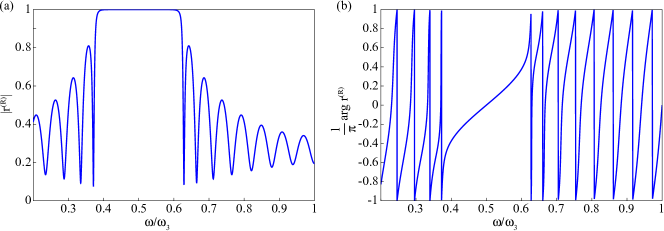
Figure 5: Absolute value (a) and argument (b) of the Bragg Mirror complex reflectivity $r^{(R)}$ for normal incidence $\theta=0$

Appendix D Bragg mirror design

The Bragg mirror is a periodic structure composed of $N$ bi-layers whose dielectric materials have refractive indexes $n^{(a)}$ and $n^{(b)}$ and thicknesses $a$ and $b$. If the layers’ thicknesses are chosen to satisfy the Bragg interference condition

$$an^{(a)}=bn^{(b)}=\frac{\pi c}{2\bar{\omega}},$$ (43)

the mirror has (for normal incidence $\theta=0$), a spectral stop-band centered at $\bar{\omega}$ whose width is proportional to the refractive index contrast $|n^{(a)}-n^{(b)}|$ Kavok . Within the stop-band the mirror reflectivity is very large, the larger $N$ the closer $|r^{(R)}(\omega)|$ to 1. As explained above in Section II, in order for one of the three fields (pump, signal and idler) to be resonant, it is necessary a very large reflectivity of the Bragg mirror at the field angular frequency, or in other words the frequency $\omega_{n}$ has to lie within the mirror stop-band. As noted above, the degenerate DR states with $\Delta\omega=0$ (where, from Eqs. (B), $\omega_{1}=\omega_{2}=\omega_{3}/2$) rigorously supports POs so that it is convenient to set the center of the mirror stop-bad at $\bar{\omega}=\omega_{3}/2$. Due to the refractive index contrast $|n^{(a)}-n^{(b)}|$, this condition assures that both signal and idler fields experience very large mirror reflectivity in a range of $\Delta\omega$ and can accordingly be resonant at the same time. On the other hand the pump frequency $\omega_{3}$ is twice the central mirror frequency $\bar{\omega}$ and requiring also the pump to resonate would require very large refractive contrast. To avoid this difficulty we have chosen to leave the pump out of resonance.

In the analysis reported in Fig.3 of the main text, we have set as pump wavelength $\lambda_{3}=780\>{\rm nm}$. For the Bragg Mirror we have chosen the refractive indexes $n_{a}=1.2$ and $n_{b}=2.5$ so that, in order to have the center of the stop-band at $\bar{\omega}=\omega_{3}/2$ we have chosen the thicknesses $a=\lambda_{3}/(2n^{(a)})=325\>{\rm nm}$ and $b=\lambda_{3}/(2n^{(b)})=156\>{\rm nm}$. We have also set $N=8$ for dealing with an efficient, feasible and compact Bragg mirror of length $d=N(a+b)=3848\>{\rm nm}$. Using the transfer matrix approach, the complex reflectivity $r^{(R)}$ (for normal incidence $\theta=0$) of the Bragg mirror which has vacuum and the dielectric at its left and right sides, respectively, is easily evaluated and we plot its absolute value and argument in panel (a) and (b), respectively, of Fig.5. Accordingly, the Bragg mirror stop-band is centered at $\omega_{3}/2$ and its spectral width is $\simeq 0.22$ $\omega_{3}$. As a consequence, if $\omega_{1}$ and $\omega_{2}$ lie within this stop-band, signal and idler waves can resonate simultaneously since $r_{1}^{(B)}=r^{(B)}(\omega_{1})$ and $r_{2}^{(B)}=r^{(B)}(\omega_{2})$ have moduli very close to $1$. The mirror stop-band width therefore yields the note-beat frequency range $0\leq\Delta\omega<0.22\omega$, which is the one considered in the analysis reported in Fig.3 of the main text. Note that $\omega_{3}$ lies outside the mirror stop-band and thus the pump field does not resonate.

Appendix E Output Fields

In order to evaluate the PO output fields $E_{n}^{\left(t\right)}$, Eqs. (B) have to be solved for a given incident pump field $E_{3}^{\left(i\right)}$. POs are characterized by $Q_{1}\neq 0$ and $Q_{2}\neq 0$ for a given $Q_{3}\neq 0$. First note that Eqs. (B) are left invariant by the gauge transformation

$$Q_{1} \to Q_{1}e^{i\theta},$$

$$Q_{2} \to Q_{2}e^{-i\theta},$$ (44)

and this implies that for a given $P_{3}$ there are infinite pairs $(Q_{1},Q_{2})$, all with the same $\Psi=\arg Q_{1}+\arg Q_{2}$. In other words, the phase difference $\Phi=\arg Q_{1}-\arg Q_{2}$ is not set by the pump field $P_{3}$. Evidently, such symmetry is spontaneously broken in actual experiments where a single pair $(Q_{1},Q_{2})$ (i.e. a single value of $\Phi$) is selected by the specific way chosen to trigger POs.

In the case of POs, the first and the complex conjugate of the second of Eqs. (B) can be casted as

$$\frac{{Q_{1}}}{{Q_{2}^{*}}}=-\frac{{\tilde{\sigma}_{23}Q_{3}}}{{\Delta_{1}}},$$

$$\frac{{Q_{1}}}{{Q_{2}^{*}}}=-\frac{{\Delta_{2}^{*}}}{{\tilde{\sigma}_{13}^{*}Q_{3}^{*}}},$$ (45)

whose consistency requires their right and left hand sides to coincide or

$$\left|{Q_{3}}\right|^{2}=\frac{{\Delta_{1}\Delta_{2}^{*}}}{{\tilde{\sigma}_{23}\tilde{\sigma}_{13}^{*}}}$$ (46)

which is the PO oscillation condition of Section II. [see Eq. (37)]. The right hand side of Eq. (46) is a positive real number if and only if the complex numbers $\Delta_{1}/\tilde{\sigma}_{23}$ and $\Delta_{2}/\tilde{\sigma}_{13}$ have the same argument $\varphi$ or

$$\Delta_{1} = \tilde{\sigma}_{23}\left|{\frac{{\Delta_{1}}}{{\tilde{\sigma}_{23}}}}\right|e^{i\varphi},$$

$$\Delta_{2} = \tilde{\sigma}_{13}\left|{\frac{{\Delta_{2}}}{{\tilde{\sigma}_{13}}}}\right|e^{i\varphi},$$ (47)

which are equivalent to Eq. (38) of Section II so that, considering only those states for which Eqs. (E) are satisfied, Eqs. (B) yield

$$\left|{\frac{{\Delta_{1}}}{{\tilde{\sigma}_{23}}}}\right|e^{i\varphi}Q_{1}+Q_{2}^{*}Q_{3} = 0,$$

$$\left|{\frac{{\Delta_{2}}}{{\tilde{\sigma}_{13}}}}\right|e^{i\varphi}Q_{2}+Q_{1}^{*}Q_{3} = 0,$$

$$\Delta_{3}Q_{3}+\tilde{\sigma}_{12}Q_{1}Q_{2} = P_{3}.$$ (48)

To solve this equation, after noting that Eqs. (E) require that $\left|\frac{Q_{1}}{Q_{2}}\right|^{2}=\left|\frac{\Delta_{2}{\tilde{\sigma}_{23}}}{{\Delta_{1}\tilde{\sigma}_{13}}}\right|$ and exploiting the above discussed gauge symmetry, we set

$$Q_{1} = \sqrt{\left|{\frac{{\Delta_{2}}}{{\tilde{\sigma}_{13}}}}\right|}\left|Q\right|e^{i\frac{1}{2}\left({\Psi+\Phi}\right)},$$

$$Q_{2} = \sqrt{\left|{\frac{{\Delta_{1}}}{{\tilde{\sigma}_{23}}}}\right|}\left|Q\right|e^{i\frac{1}{2}\left({\Psi-\Phi}\right)},$$ (49)

where we have used the symbol $|Q|$ to stress than this quantity is real. Inserting Eqs. (E) into Eqs. (E) yield

$$Q_{3} = -\sqrt{\left|{\frac{{\Delta_{1}\Delta_{2}}}{{\tilde{\sigma}_{23}\tilde{\sigma}_{13}}}}\right|}e^{i\left({\Psi+\varphi}\right)},$$

$$\left|Q\right|^{2}+\frac{{\Delta_{3}}}{{\tilde{\sigma}_{12}}}\sqrt{\left|{\frac{{\tilde{\sigma}_{23}\tilde{\sigma}_{13}}}{{\Delta_{1}\Delta_{2}}}}\right|}e^{-i\Psi}Q_{3} = \sqrt{\left|{\frac{{\tilde{\sigma}_{23}\tilde{\sigma}_{13}}}{{\Delta_{1}\Delta_{2}}}}\right|}\frac{{P_{3}}}{{\tilde{\sigma}_{12}}}e^{-i\Psi}.$$ (50)

Note that the first two of Eqs. (E) both reduces to the first of Eqs. (E) through the change of variables given by Eqs. (E) and this is a consequence of the necessary Eq. (E). Substituting $Q_{3}$ from the first of Eqs. (E) into the second we get

$$\left|Q\right|^{2}-\frac{{\Delta_{3}}}{{\tilde{\sigma}_{12}}}e^{i\varphi}=\sqrt{\left|\frac{{\tilde{\sigma}_{23}\tilde{\sigma}_{13}}}{{\Delta_{1}\Delta_{2}}}\right|}\frac{{P_{3}}}{{\tilde{\sigma}_{12}}}e^{-i\Psi},$$ (51)

which is a single complex equation for $|Q|$ and $\Psi$. After equating the square-moduli of the left and right sides of this equation we get

$$\left|Q\right|^{4}-2{\mathop{\rm Re}\nolimits}\left({\frac{{\Delta_{3}}}{{\tilde{\sigma}_{12}}}e^{i\varphi}}\right)\left|Q\right|^{2}+\left(\left|{\frac{{\Delta_{3}}}{{\tilde{\sigma}_{12}}}e^{i\varphi}}\right|^{2}-\left|\frac{{\tilde{\sigma}_{23}\tilde{\sigma}_{13}}}{{\Delta_{1}\Delta_{2}}}\right|\left|{\frac{{P_{3}}}{{\tilde{\sigma}_{12}}}}\right|^{2}\right)=0,$$ (52)

which is a biquadratic equation for $\left|Q\right|$ whose solutions are

$$\left|Q\right|=\sqrt{{\mathop{\rm Re}\nolimits}\left({\frac{{\Delta_{3}}}{{\tilde{\sigma}_{12}}}e^{i\varphi}}\right)+\xi\sqrt{\left|\frac{{\tilde{\sigma}_{23}\tilde{\sigma}_{13}}}{{\Delta_{1}\Delta_{2}}}\right|\left|{\frac{{P_{3}}}{{\tilde{\sigma}_{12}}}}\right|^{2}-{\mathop{\rm Im}\nolimits}^{2}\left({\frac{{\Delta_{3}}}{{\tilde{\sigma}_{12}}}e^{i\varphi}}\right)}},$$ (53)

where $\xi=\pm 1$. Note that, due to the $\xi$ factor, generally there are two $|Q|$ corresponding to a $|P_{3}|$ and hence bistable POs can in principle occur. In addition, it is fundamental stressing that $|Q|$ is real and hence Eq. (53) provides its value only if the arguments of the square roots are positive. Before discussing the range of $|P_{3}|$ where this is the case (see below), we assume $|Q|$ real and we deduce the output field amplitudes. Equation (51) yields

$$e^{i\Psi}=\sqrt{\left|{\frac{{\tilde{\sigma}_{23}\tilde{\sigma}_{13}}}{{\Delta_{1}\Delta_{2}}}}\right|}\frac{\displaystyle{P_{3}}}{\displaystyle{\tilde{\sigma}_{12}\left({\left|Q\right|^{2}-\frac{{\Delta_{3}}}{{\tilde{\sigma}_{12}}}e^{i\varphi}}\right)}},$$ (54)

which is consistent since the modulus of its right hand side, due to Eq. (53), is equal to $1$. Hence Eqs. (E) and the first of Eqs. (E) eventually yield

$$Q_{1} = \zeta\left|{\frac{\displaystyle{\Delta_{2}\tilde{\sigma}_{23}}}{\displaystyle{\Delta_{1}\tilde{\sigma}_{13}}}}\right|^{1/4}\sqrt{\frac{\displaystyle{P_{3}}}{\displaystyle{\tilde{\sigma}_{12}\left({\left|Q\right|^{2}-\frac{{\Delta_{3}}}{{\tilde{\sigma}_{12}}}e^{i\varphi}}\right)}}}e^{i\frac{\Phi}{2}}\left|Q\right|,$$

$$Q_{2} = \zeta\left|{\frac{\displaystyle{\Delta_{1}\tilde{\sigma}_{13}}}{\displaystyle{\Delta_{2}\tilde{\sigma}_{23}}}}\right|^{1/4}\sqrt{\frac{\displaystyle{P_{3}}}{\displaystyle{\tilde{\sigma}_{12}\left({\left|Q\right|^{2}-\frac{{\Delta_{3}}}{{\tilde{\sigma}_{12}}}e^{i\varphi}}\right)}}}e^{-i\frac{\Phi}{2}}\left|Q\right|,$$

$$Q_{3} = \frac{\displaystyle{P_{3}}}{\displaystyle{\tilde{\sigma}_{12}\left({\left|Q\right|^{2}-\frac{{\Delta_{3}}}{{\tilde{\sigma}_{12}}}e^{i\varphi}}\right)}}e^{i\left({\varphi+\pi}\right)},$$ (55)

where $\zeta=\pm 1$ and the principal branch is assumed for all the complex square-roots.

Note that the output fields of Eqs. (E) satisfy Eq. (46) so that they describe all the possible cavity POs whenever they exist or, in other words, whenever $|Q|$ of Eq. (53) is a positive real number. Such requirement evidently sets a range for the input pump intensity $|P_{3}|^{2}$ and there are four different cases corresponding to the two values of $\xi$ and of the two signs of ${\mathop{\rm Re}\nolimits}\left({\frac{{\Delta_{3}}}{{\tilde{\sigma}_{12}}}e^{i\varphi}}\right)$. The results of this analysis are reported in the following table.

$$\begin{array}[]{c | c | c }&{\mathop{\rm Re}\nolimits}\left({\frac{{\Delta_{3}}}{{\tilde{\sigma}_{12}}}e^{i\varphi}}\right)>0&{\mathop{\rm Re}\nolimits}\left({\frac{{\Delta_{3}}}{{\tilde{\sigma}_{12}}}e^{i\varphi}}\right)<0\\ \hline\cr&&\\ \xi=1&\left|{P_{3}}\right|^{2}>\left(\left|{P_{3}}\right|^{2}\right)_{-}&\left|{P_{3}}\right|^{2}>\left(\left|{P_{3}}\right|^{2}\right)_{th}\\ &&\\ \hline\cr&&\\ \xi=-1&\left(\left|{P_{3}}\right|^{2}\right)_{-}<\left|{P_{3}}\right|^{2}<\left(\left|{P_{3}}\right|^{2}\right)_{th}&{\rm no}\>|P_{3}|^{2}\\ &&\\ \hline\cr\end{array}$$

Here we have set

$$\left(\left|{P_{3}}\right|^{2}\right)_{-}=\left|{\frac{{\Delta_{1}\Delta_{2}}}{{\tilde{\sigma}_{23}\tilde{\sigma}_{13}}}}\right|{\mathop{\rm Im}\nolimits}^{2}\left({\Delta_{3}\frac{{\left|{\tilde{\sigma}_{12}}\right|}}{{\tilde{\sigma}_{12}}}e^{i\varphi}}\right)<{\left|{\frac{{\Delta_{1}\Delta_{2}}}{{\tilde{\sigma}_{23}\tilde{\sigma}_{13}}}}\right|\left|{\Delta_{3}}\right|^{2}}=\left(\left|{P_{3}}\right|^{2}\right)_{th}.$$ (56)

Therefore at each state where PO can occur (i.e. at a each point of the surface $\Sigma$) the scenario is the following one. If ${\mathop{\rm Re}\nolimits}\left({\frac{{\Delta_{3}}}{{\tilde{\sigma}_{12}}}e^{i\varphi}}\right)<0$, there is only one PO (with $\xi=1$) that effectively starts when Eq. (39) is satisfied, thus confirming the analysis of Section III. On the other hand, if ${\mathop{\rm Re}\nolimits}\left({\frac{{\Delta_{3}}}{{\tilde{\sigma}_{12}}}e^{i\varphi}}\right)>0$ the scenario changes qualitatively since in this case there are two allowed POs (with $\xi=1$ and $\xi=-1$) when $\left(\left|{P_{3}}\right|^{2}\right)_{-}<\left|{P_{3}}\right|^{2}<\left(\left|{P_{3}}\right|^{2}\right)_{th}$ and a single PO (with $\xi=1$) when Eq. (39) is satisfied. As a consequence in this case POs also exist below the threshold.

In order to grasp the reason why the sub-threshold POs have not been entailed in Section III, note that in the case ${\mathop{\rm Re}\nolimits}\left({\frac{{\Delta_{3}}}{{\tilde{\sigma}_{12}}}e^{i\varphi}}\right)>0$, if $\left|{P_{3}}\right|^{2}=\left(\left|{P_{3}}\right|^{2}\right)_{-}$, Eq. (53) implies that $\left|Q\right|=\sqrt{{\mathop{\rm Re}\nolimits}\left({\frac{{\Delta_{3}}}{{\tilde{\sigma}_{12}}}e^{i\varphi}}\right)}\neq 0$ so that $Q_{1}\neq 0$ and $Q_{2}\neq 0$. In other words in this situation the signal and idler fields do not vanish at the threshold and accordingly this case is ruled out from the reasoning of Section III where the threshold has been obtained for PO oscillation starting from the linear regime. In a realistic experiment PO is switched on starting from the linear regime, with the intensity threshold given by Eq. (39). However, once PO ignites, by changing the pump intensity, incidence angle $\theta$, or the cavity length, we argue that one can in principle access sub-threshold PO states. In every design considered in the main paper we have focused on the case ${\mathop{\rm Re}\nolimits}\left({\frac{{\Delta_{3}}}{{\tilde{\sigma}_{12}}}e^{i\varphi}}\right)<0$, where sub-threshold PO does not occur.

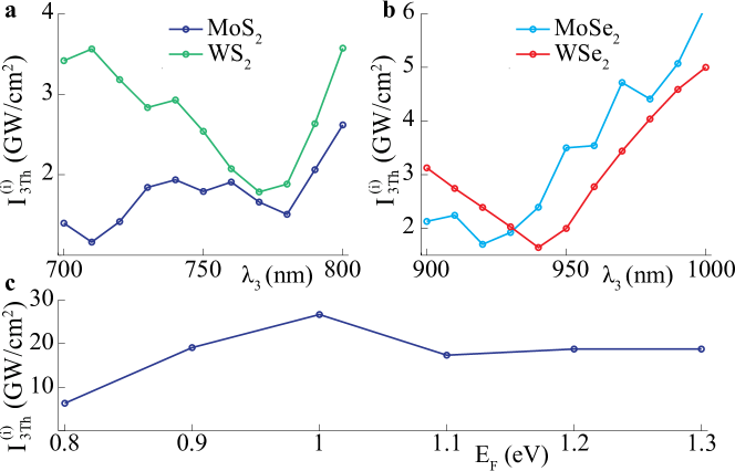
Figure 6: Parametric Oscillation Thresholds. a,b Pump wavelength $\lambda_{3}$ dependence of the pump intensity thresholds for parametric oscillators embedding MoS₂, WS₂ (a) and MoSe₂, WSe₂ (b). c Pump intensity threshold of a parametric oscillator embedding MoS₂ as a function of the Fermi level. The thresholds are associated to non-degenerate ($\Delta\omega=0$) POs and they have been calculated for cavities whose length $L$ is equal to the pump wavelength $\lambda_{3}$.

Appendix F Pump intensity thresholds

In Fig. 6 we compare the calculated pump intensity thresholds versus the pump wavelength $\lambda_{3}$ for parametric oscillators embedding MoS₂, WS₂ (Fig. 6a) and MoSe₂, WSe₂ (Fig. 6b). Note that, while the minimal pump intensity threshold occurs at $\lambda_{3}\approx 780$ nm for MoS₂ and WS₂, it shifts to $\lambda_{3}\approx 940$ nm for MoSe₂ and WSe₂. None of the ML-TMDs examined enables feasible PO with low pump intensity threshold at optical frequencies owing to the enlarged absorption in this frequency range, which is the main responsible for oscillation quenching. In addition, at optical frequencies such materials exhibit exciton resonances UBS2014 (not taken into account in our theoretical approach) that are also detrimental for POs owing to the enhanced absorption they are accompanied with. In Fig. 6c we plot the pump intensity threshold as a function of the Fermi level of MoS₂, showing that it can be increased efficiently. Thus, the external gate voltage quenches POs when the optical pump is fixed and fast modulation of the output signal and idler fields can be achieved with novel parametric oscillators embedding ML-TMDs.

References

- (1) P. A. Franken, A. E. Hill, C. W. Peters, and G. Weinreich, “Generation of Optical Harmonics,´´ Phys. Rev. Lett. 7, 118 - 119 (1961).
- (2) T. A. Birks, W. J. Wadsworth, P. St.J. Russell, “Supercontinuum generation in tapered fibers,´´ Opt. Lett. 25, 1415 - 1417 (2000).
- (3) G. I. Stegeman, D. J. Hagan, and L. Torner, “ cascading phenomena and their applications to all-optical signal processing, mode-locking, pulse compression and solitons,´´ Opt. Quant. Electron. 28, 1691 - 1740 (1996).
- (4) C. Koos, P. Vorreau, T. Vallaitis, P. Dumon, W. Bogaerts, R. Baets, B. Esembeson, I. Biaggio, T. Michinobu, F. Diederich, W. Freude, and J. Leuthold, “All-optical high-speed signal processing with silicon–organic hybrid slot waveguides,´´ Nat. Photon. 3, 216 - 219 (2009).
- (5) P. G. Kwiat, K. Mattle, H. Weinfurter, A. Zeilinger, A. V. Sergienko, and Y. Shih, “New High-Intensity Source of Polarization-Entangled Photon Pairs,´´ Phys. Rev. Lett. 75, 4337 - 4341 (1995).
- (6) R. M. Stevenson, R. J. Young, P. Atkinson, K. Cooper, D. A. Ritchie, and A. J. Shields, “A semiconductor source of triggered entangled photon pairs,´´ Nature 439, 179 - 182 (2006).
- (7) J. A. Giordmaine and R. C. Miller, “Tunable Coherent Parametric Oscillation in LiNbO3 at Optical Frequencies,´´ Phys. Rev. Lett. 14, 973 - 976 (1965).
- (8) A. Yariv and W. H, Louisell, “Theory of the Optical Parametric Oscillator,´´ IEEE J. Quant. Electron. 9, 418 - 424 (1966).
- (9) S. J. Brosnan and R. L. Byer, “Optical Parametric Oscillator Threshold and Linewidth Studies,´´ IEEE J. Quant. Electron. 15, 415 - 431 (1979).
- (10) R. C. Eckardt, C. D. Nabors, W. J. Kozlovsky, and R. L. Byer, “Optical parametric oscillator frequency tuning and control,´´ J. Opt. Soc. Am. B 8, 646 - 667 (1991).
- (11) T. Debuisschert, A. Sizmann, E. Giacobino, and C. Fabre, “Type-II continuous-wave optical parametric oscillators: oscillation and frequency-tuning characteristics,´´ J. Opt. Soc. Am. B 10, 1668 - 1680 (1993).
- (12) C. Fabre, P. F. Cohadon, and C. Schwob, “CW optical parametric oscillators: single mode operation and frequency tuning properties,´´ Quantum Semiclass. Opt. 9, 165 - 172 (1997).
- (13) J. S. Levy, A. Gondarenko, M. A. Foster, A. C. Turner-Foster, A. L. Gaeta, and M. Lipson, “CMOS-compatible multiple-wavelength oscillator for on-chip optical interconnects,´´ Nat. Photon. 4, 37 - 40 (2010).
- (14) L. Razzari, D. Duchesne, M. Ferrera, R. Morandotti, S. Chu, B. E. Little, and D. J. Moss, “CMOS-compatible integrated optical hyperparametric oscillator,´´ Nat. Photon. 4, 41 - 45 (2010).
- (15) L.-A. Wu, M. Xiao, and H. J. Kimble, “Squeezed states of light from an optical parametric oscillator,´´ J. Opt. Soc. Am. B 4, 1465 - 1475 (1987).
- (16) Y. J. Lu and Z. Y. Ou, “Optical parametric oscillator far below threshold: Experiment versus theory,´´ Phys. Rev. A 62, 033804 (2000).
- (17) C. Ciuti, P. Schwendimann and A. Quattropani, “Theory of polariton parametric interactions in semiconductor microcavities,´´ Semicond. Sci. Technol. 18, S279 – S293 (2003).
- (18) C. Diederichs, J. Tignon, G. Dasbach, C. Ciuti, A. Lemaitre, J. Bloch, Ph. Roussignol and C. Delalande, “Parametric oscillation in vertical triple microcavities´´ Nature 440, 904 - 907 (2006).
- (19) M. Abbarchi, V. Ardizzone, T. Lecomte, A. Lemaıtre, I. Sagnes, P. Senellart, J. Bloch, P. Roussignol, and J. Tignon, “One-dimensional microcavity-based optical parametric oscillator: Generation of balanced twin beams in strong and weak coupling regime,´´ Phys. Rev. B 83, 201310(R) (2011).
- (20) J. A. Giordmaine, “Mixing of Light Beams in Crystals,´´ Phys. Rev. Lett. 8, 19 – 20 (1962).
- (21) K. L. Vodopyanov, O. Levi, P. S. Kuo, T. J. Pinguet, J. S. Harris, M. M. Fejer, B. Gerard, L. Becouarn, and E. Lallier, “Optical parametric oscillation in quasi-phase-matched GaAs,´´ Opt. Lett. 29, 1912 – 1914 (2004).
- (22) C. Canalias, and V. Pasiskevicius, “Mirrorless optical parametric oscillator,´´ Nature Photonics 1 459 - 462 (2007).
- (23) P. G. Savvidis, J. J. Baumberg, R. M. Stevenson, M. S. Skolnick, D. M. Whittaker, and J. S. Roberts, “Angle-Resonant Stimulated Polariton Amplifier,´´ Phys. Rev. Lett. 84, 1547 – 1550 (2000).
- (24) C. Ciuti, P. Schwendimann, B. Deveaud, and A. Quattropani, ´´Theory of the angle-resonant polariton amplifier,´´ Phys. Rev. B 62, R4825–-R4828 (2000).
- (25) Z. D. Xie, X. J. Lv, Y.H. Liu, W. Ling, Z. L. Wang, Y. X. Fan, and S. N. Zhu, ´´Cavity Phase Matching via an Optical Parametric Oscillator Consisting of a Dielectric Nonlinear Crystal Sheet,´´ Phys. Rev. Lett. 106, 083901 (2011).
- (26) Q. Clément, J.-M. Melkonian, M. Raybaut, J.-B. Dherbecourt, A. Godard, B. Boulanger, and M. Lefebvre, ´´Ultrawidely tunable optical parametric oscillators based on relaxed phase matching: theoretical analysis,´´ J. Opt. Soc. Am. B 32, 52 - 68 (2015).
- (27) K. F. Mak, C. Lee, J. Hone, J. Shan, and T. F. Heinz, “Atomically Thin : A New Direct-Gap Semiconductor,´´ Phys. Rev. Lett. 105, 136805 (2010).
- (28) A. Splendiani, L. Sun, Y. Zhang, T. Li, J. Kim, C. Y. Chim, G. Galli, and F. Wang, “Emerging photoluminescence in monolayer ,´´Nano Lett. 10 1271 - 1275 (2010).
- (29) Q. H. Wang, K. Kalantar-Zadeh, A. Kis, J. N. Coleman, and M. S. Strano, “Electronics and optoelectronics of two-dimensional transition metal dichalcogenides,´´ Nat. Nanotechnol. 7, 699 - 712 (2012).
- (30) Z. Sun, A. Martinez, and F. Wang, “Optical modulators with 2D layered materials,´´ Nat. Photon. 10, 227 - 238 (2016).
- (31) N. Kumar, S. Najmaei, Q. Cui, F. Ceballos, P. M. Ajayan, J. Lou, and H. Zhao, “Second harmonic microscopy of monolayer MoS2,´´Phys. Rev. B 87, 161403(R) (2013).
- (32) Y. Li, Y. Rao, K. F. Mak, Y. You, S. Wang, C. R. Dean, T. F. Heinz, “Probing symmetry properties of few-layer and h-BN by optical second-harmonic generation,´´ Nano Lett. 13, 3329 - 3333 (2013).
- (33) L. M. Malard, T. V. Alencar, A. P. M. Barboza, K. F. Mak, and A. M. de Paula, “Observation of intense second harmonic generation from atomic crystals,´´ Phys. Rev. B 87, 201401(R) (2013).
- (34) C. Janisch, Y. Wang, D. Ma, N. Mehta, A. L. Elias, N. Perea-Lopez, M. Terrones, V. Crespi, and Z. Liu, Sci. Rep. 4, 5530 (2014).
- (35) C. T. Le, D. J. Clark, F. Ullah, V. Senthilkumar, J. I. Jang, Y. Sim, M.-J. Seong, K.-H. Chung, H. Park, and Y. S. Kim, “Nonlinear optical characteristics of monolayer ,´´ Ann. Phys. 528, 551 - 559 (2016).
- (36) G.-B. Liu, W.-Y. Shan, Y. Yao, W. Yao, and D. Xiao, “Three-band tight-binding model for monolayers of group-VIB transition metal dichalcogenides,´´ Physical Review B 88, 085433 (2013).
- (37) See Supplemental Material for more details on the technical aspects of the theory.
- (38) M. M. Ugeda, A. J. Bradley, S.-F. Shi, F. H. da Jornada, Y. Zhang, D. Y. Qiu, W. Ruan, S.-K. Mo, Z. Hussain, Z.-X. Shen, F. Wang, S. G. Louie, and M. F. Crommie, “Giant bandgap renormalization and excitonic effects in a monolayer transition metal dichalcogenide semiconductor´´, Nat. Mater. 13, 1091-1095 (2014).
- (39) M. Selig, G. Berghäuser, A. Raja, P. Nagler, C. Schüller, T. F. Heinz, T. Korn, A. Chernikov, E. Malic, and A. Knorr, “Excitonic linewidth and coherence lifetime in monolayer transition metal dichalcogenides´´, Nat. Commun 7, 13279 (2016).
- (40) G.-B. Liu, W.-Y. Shan, Y. Yao, W. Yao, and D. Xiao, “Three-band tight-binding model for monolayers of group-VIB transition metal dichalcogenides,´´ Physical Review B 88, 085433 (2013).
- (41) M. M. Ugeda, A. J. Bradley, S.-F. Shi, F. H. da Jornada, Y. Zhang, D. Y. Qiu, W. Ruan, S.-K. Mo, Z. Hussain, Z.-X. Shen, F. Wang, S. G. Louie, and M. F. Crommie, “Giant bandgap renormalization and excitonic effects in a monolayer transition metal dichalcogenide semiconductor,´´ Nat. Mater. 13, 1091 - 1095 (2014).
- (42) F. Ceballos, Q. Cui, M. Z. Bellusa, and H. Zhao, “Exciton formation in monolayer transition metal dichalcogenides,´´ Nanoscale 8, 11681 - 11688 (2016).
- (43) X. Yin, Z. Ye, D. A. Chenet, Y. Ye, K. O’Brien, J. C. Hone, X. Zhang, “Edge Nonlinear Optics on a MoS2 Atomic Monolayer´´, Science 344, 488–490 (2014).
- (44) A. V. Kavokin, J. J. Baumberg, G. Malpuech and F. P. Laussy, Microcavities (Oxford University Press, USA 2008)