A real-frequency solver for the Anderson impurity model based on bath optimization and cluster perturbation theory

Abstract

Recently solvers for the Anderson impurity model (AIM) working directly on the real-frequency axis have gained much interest. A simple and yet frequently used impurity solver is exact diagonalization (ED), which is based on a discretization of the AIM bath degrees of freedom. Usually, the bath parameters cannot be obtained directly on the real-frequency axis, but have to be determined by a fit procedure on the Matsubara axis. In this work we present an approach where the bath degrees of freedom are first discretized directly on the real-frequency axis using a large number of bath sites ($\approx 50$). Then, the bath is optimized by unitary transformations such that it separates into two parts that are weakly coupled. One part contains the impurity site and its interacting Green’s functions can be determined with ED. The other (larger) part is a non-interacting system containing all the remaining bath sites. Finally, the Green’s function of the full AIM is calculated via coupling these two parts with cluster perturbation theory.

1 Introduction

The single-orbital Anderson impurity model (AIM) [1] can be represented exactly by an interacting site coupled to a bath of infinitely many non-interacting sites. In approaches based on exact diagonalization (ED), the number of sites in the interacting system is restricted, and thus the bath needs to be truncated [2; 3; 4]. This is a delicate step, because no unique procedure exists. Different ways are used, e.g., fits on the Matsubara axis or continuous fraction expansions [3; 5; 6].

Various methods improving on ED have been presented in recent years, e.g., the variational exact diagonalization [7], the distributional exact diagonalization [8] and methods based on a restriction of the basis states [9; 10; 11; 12; 13]. Another way of going beyond ED is the use of cluster perturbation theory (CPT) [14; 15; 16], i.e. the more advanced variational cluster approximation (VCA) [17; 18; 19], as a solver for the AIM [20; 21].

From now on, we assume a single-orbital AIM coupled to a finite but large bath of $L-1$ non-interacting sites. The basic idea of using CPT as an impurity solver is to separate the $L$-site AIM into a cluster of size $L_{C}$, which includes the impurity site and $L_{C}-1$ bath sites, and a non-interacting system consisting of the remaining bath sites. In general, the non-interacting Green’s function is specified by the Hamiltonian $H^{0}$, that is a matrix in orbital space of size $L\times L$. For illustration purposes (see the sketch in Fig. 1), we denote the upper left $L_{C}\times L_{C}$ block in $H^{0}$ as the interacting cluster, subsequently $H^{0}_{C}$. The remaining, lower $(L-L_{C})\times(L-L_{C})$ block describes the remainder of the bath, subsequently $H^{0}_{R}$. Additionally, there are two off-diagonal blocks $T$ connecting $H^{0}_{C}$ and $H^{0}_{R}$. The onsite Hubbard interaction $H_{U}=Un_{I,\uparrow}n_{I,\downarrow}$, where $I$ labels the impurity site, is now added to the cluster Hamiltonian, $H_{C}=H_{C}^{0}+H_{U}$. There are no interactions in the bath degrees of freedom, hence $H_{R}^{0}$ remains unchanged.

In CPT both Hamiltonians ($H_{C}$ and $H^{0}_{R}$) are solved exactly for their single-particle Green’s functions $G_{C}(\omega)$ and $G_{R}(\omega)$. To obtain $G_{C}(\omega)$ we use the Lanczos procedure at zero temperature [22; 23]. Note that $G_{R}(\omega)=G^{0}_{R}(\omega)$, as the remainder of the bath is a non-interacting system. Subsequently, the two systems are joined to yield the single-particle Green’s function of the full system $G(\omega)$ via the CPT relation [15]

$$G^{-1}(\omega) =\left(\begin{array}[]{cc}G_{C}(\omega)&0\\ 0&G_{R}(\omega)\\ \end{array}\right)^{-1}-V\,\mbox{,}$$ (3)

where $V$ is a $L\times L$ coupling matrix consisting only of the $T$ blocks. Eq. 3 is exact in the case of a non-interacting system ($U=0$). In the interacting case, the CPT relation is no longer exact, but a result of perturbation theory in $V$. CPT approximates the self-energy of the full system by the self-energy of the interacting cluster.

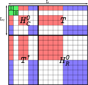
Figure 1: Splitting of the Hamiltonian $H^{0}$ into an interacting cluster $H^{0}_{C}$ of $L_{C}=6$ sites, the remaining reservoir $H^{0}_{R}$ and the coupling of those two system $T$. In the specific example of a particle-hole symmetric system the unitary updates are performed in the space of negative energies (red) and equivalently in the space of positive energies (blue). No non-zero matrix elements are generated in the white blocks by the two-dimensional rotation matrices used in this work. The diagonal blocks from top to bottom represent: 1) the impurity, 2) the zero mode inside the cluster, 3) two negative modes inside the cluster, 4) two positive modes inside the cluster, 5) the remaining negative modes in the reservoir and 6) the remaining positive modes in the reservoir.

In general, the non-interacting bath can always be transformed to a tridiagonal representation via a Lanczos tridiagonalization, yielding a chain representation of the AIM. This representation straight forwardly allows to define the separation of the interacting cluster and the remainder of the bath. However, the situation is not so clear in other representations. Consider for example the case of a star geometry, where all bath sites couple directly to the impurity site. Incorporating just a random set of these star sites into the interacting cluster will lead to a poor discretization of the bath, and hence a poor self-energy.

Any unitary transformation on the non-interacting bath degrees of freedom leaves the physics of the interacting AIM invariant. However, such a transformation will influence the self-energy of the interacting cluster significantly, since it changes the cluster Hamiltonian $H_{C}$. Additionally, such transformations will also alter the off-diagonal block $T$, rendering the resulting perturbation in some cases larger than in others. There exist an infinite number of representations which all describe the non-interacting bath exactly and which are related via unitary transformations. However, the CPT method itself suggests which baths might be the best: Those which “minimize” the off-diagonal perturbative elements in $T$. The key idea of this work is to use unitary transformations to find those bath representations with minimal couplings between the cluster and the remainder of the bath.

In the following, we outline a way to construct CPT-favorable bath representations in Sec. 2, and present results for a $L=64$ AIM with a semi-circular particle-hole symmetric bath in Sec. 3.

2 Method

The general form of the non-interacting Hamiltonian for an $L$-site AIM is

$$H_{0} =\epsilon_{I}c^{\dagger}_{I}c_{I}^{\phantom{{\dagger}}}+\sum\limits_{i=1}^{L-1}\left(t_{iI}c^{\dagger}_{i}c_{I}^{\phantom{{\dagger}}}+{\rm h.c.}\right)+\sum\limits_{i,j=1}^{L-1}t_{ij}c^{\dagger}_{i}c_{j}^{\phantom{{\dagger}}}\ ,$$ (4)

where the impurity is denoted by the index $I$ and the $L-1$ bath sites by $i$ and $j$. We omit the spin indices. To obtain $H_{0}$ for an $L$-site system one can use a star representation, where each bath site couples only to the impurity site. Then, the parameters of $H_{0}$ can be determined by a discretization of the non-interacting bath DOS into equally spaced intervals. Each interval is represented by a delta peak, where the energy positions of the delta peaks correspond to the on-site energies and the hopping parameters are obtained from the spectral weights in the intervals. Of course, the higher the number of bath sites the better the result of this discretization.

Under a unitary transformation $R$, performed in the bath only, with $c_{i}^{\phantom{{\dagger}}}=\sum_{\alpha}R_{i\alpha}d_{\alpha}^{\phantom{{\dagger}}}$ and $c_{i}^{\dagger}=\sum_{\alpha}d_{\alpha}^{\dagger}R^{*}_{\alpha i}$, where $RR^{\dagger}=11$, the transformed Hamiltonian reads

$$H^{\prime}_{0} =\epsilon_{I}c^{\dagger}_{I}c_{I}^{\phantom{{\dagger}}}+\sum\limits_{\alpha=1}^{L-1}\left(h_{\alpha I}d_{\alpha}^{\dagger}c_{I}^{\phantom{{\dagger}}}+{\rm h.c.}\right)+\sum\limits_{\alpha,\beta=1}^{L-1}h_{\alpha\beta}d_{\alpha}^{\dagger}d_{\beta}^{\phantom{{\dagger}}}\ .$$ (5)

The parameters of the Hamiltonian transform like $h_{\alpha I}=\sum_{i}R^{*}_{\alpha i}t_{iI}$ and $h_{\alpha\beta}=\sum_{i,j}R^{*}_{\alpha i}t_{ij}R_{j\beta}$. Such a transformation leaves the impurity state $I$ and consequently $\epsilon_{I}$ invariant.

We define an “energy” of a certain bath representation via the 2-norm of the off-diagonal blocks $T$

$$E=\frac{1}{N_{T}}\sum\limits_{i,j}|T_{ij}|^{2}\,\mbox{,}$$ (6)

where the number of elements in $T$ is $N_{T}=L_{C}\cdot(L-L_{C})$. Transformations on the bath degrees of freedom included in the interacting cluster do not influence the resulting self-energy. The same is true for transformations performed only in the remainder of the bath. This imposes a constraint on the energy $E$, namely, it has to be invariant with respect to such transformations, which is indeed fulfilled by the 2-norm.

The aim is now to find an optimal bath representation for CPT by minimizing the energy $E$. Since the configuration space of $T_{ij}$ is high dimensional, we use a Monte Carlo procedure. Initially, we perform global updates in all dimensions with random rotation matrices to obtain a randomized starting representation of $H_{0}$. Then, we move through the space of possible $H_{0}$ by proposing random local updates $R$. In general, any unitary update would be allowed, but here we restrict ourselves to two-dimensional rotation matrices for the local updates

$$R=\left(\begin{array}[]{ccccccccc}1&0&\ldots&0&0&\ldots&0&\ldots&0\\ 0&1&\ldots&0&0&\ldots&0&\ldots&0\\ \ldots&\ldots&\ldots&\ldots&\ldots&\ldots&\ldots&\ldots&0\\ 0&0&\ldots&\cos\left(\phi\right)&0&\ldots&-\sin\left(\phi\right)&\ldots&0\\ 0&0&\ldots&0&1&\ldots&0&\ldots&0\\ \ldots&\ldots&\ldots&\ldots&\ldots&\ldots&\ldots&\ldots&0\\ 0&0&\ldots&\sin\left(\phi\right)&0&\ldots&\cos\left(\phi\right)&\ldots&0\\ \ldots&\ldots&\ldots&\ldots&\ldots&\ldots&\ldots&\ldots&\ldots\\ 0&0&\ldots&0&0&\ldots&0&\ldots&1\\ \end{array}\right)$$

A local update matrix $R(i,j,\phi)$ is drawn by choosing two random integers $i,j\in[1,L-1]$ representing the plane of rotation and one rotation angle $\phi\in[0,2\pi[$. A new representation with energy $E^{\prime}$ is accepted with probability $p=\text{min}\left(1,e^{-\gamma(E^{\prime}-E)}\right)$. We use simulated annealing to obtain low-energy CPT bath representations by increasing the parameter $\gamma$.

Although bath rotations leave the particle-hole symmetry invariant on the $L$-site $H_{0}$, they destroy it on the $L_{C}$-site cluster. Therefore, as shown in Fig. 1, we split the bath sites into an equal amount of positive (blue elements) and negative energy (red elements) sites and one zero mode (green 0). Updates are performed simultaneously on the positive and negative modes which leaves the whole bath, the bath in the cluster as well as the remaining bath particle-hole invariant. To avoid a Kramers-degenerate ground state, clusters with an even number of sites $L_{C}$ are chosen. This implies that one bath site (the zero mode) is exactly located at zero energy. Zero mode updates cannot be achieved by two-dimensional rotations without breaking the particle-hole symmetry of the cluster, but would rather require special unitary transformations involving at least three bath sites. For the proof of concept presented here, we refrain from updating the zero mode, i.e. the green elements in Fig. 1 do not change. Hence, the zero mode coupling is determined by the initial discretization of the system. Although this restricts the space of trial bath representations, we leave the zero mode updates for future works.

Next to the energy $E$ (Eq. 6), which reflects the magnitude of the perturbation, we evaluate the influence of the CPT truncation by comparing the non-interacting single-particle impurity Green’s function of the full system $G^{I}_{0}(\omega)$ to the one considering only the sites in the cluster $G^{I}_{0,C}(\omega)$. The resulting quantity

$$\chi^{2}_{C}=\int d\omega\left|G^{I}_{0}(\omega+i\eta)-G^{I}_{0,C}(\omega+i\eta)\right|^{2}\,\mbox{,}$$ (7)

reflects the ability of the $L_{C}$ cluster sites to represent the bath degrees of freedom. A-priori a positive correlation of $E$ and $\chi^{2}_{C}$ is not ensured but expected. We emphazise that $\chi^{2}_{C}$ is not used in the algorithm, but only serves as a measurement for the quality of the bath optimization. A numerical broadening of $\eta=$0.02\text{\,}\mathrm{eV}$$ is used to evaluate Eq. 7.

To asses the quality of the optimization scheme we also perform plain ED calculations for a truncated $L=10$ system. The Hamiltonian of this 10-sites system (with the Green’s function $G^{I}_{0,ED}(i\omega_{n})$) is obtained by fitting $G^{I}_{0}\left(i\omega\right)$ on the Matsubara axis with the cost function

$$\chi^{2}_{ED}=\sum\limits_{n}W_{n}\left|G^{I}_{0}(i\omega_{n})^{-1}-G^{I}_{0,ED}(i\omega_{n})^{-1}\right|^{2}\,\mbox{.}$$ (8)

We employ the simplex search method by Lagarias et al. [24] and impose particle-hole symmetry to reduce the number of fit parameters. A Matsubara grid with 1024 points at a fictitious temperature corresponding to $\beta=$100\text{\,}\mathrm{eV}^{-1}$$ is used, but the ED solution itself is obtained at zero temperature. The cost function Eq. 8 is a heuristic choice and can also take various other forms, e.g. with a different definition of the distance or a different weight $W_{n}$ (we set $W_{n}=1/\omega_{n}$) [5; 6] . This leads to an ad-hoc determination of the bath parameters and introduces some ambiguity to the solution of the AIM. For a given number of bath sites also the discretization on the real-frequency axis is not uniquely defined, e.g. we could use unequally spaced energy intervals. In contrast to ED, where usually only a small number of bath sites is fitted on the Matsubara axis via the minimization of Eq. 8, the discretization on the real-frequency axis can be easily performed for a large number of sites. Indubitably, the ambiguities in determining the AIM parameters are less severe for larger system sizes.

3 Results

Here, we discuss a single interacting impurity in a particle-hole symmetric semi-circular bath with a half-bandwidth of $1\text{\,}\mathrm{eV}$. For the bath optimization we use a discretized system with a total number of $L=64$ sites and an interacting cluster of $L_{C}=10$. The interacting cluster includes the impurity site, one zero mode, and four additional positive and negative bath sites each.

Fig. 2 shows that smaller perturbative elements $E$ correlate positively with smaller $\chi^{2}_{C}$, indicating a better representation of the non-interacting bath by the sites contained in the interacting cluster. We compare intermediate bath representations (black crosses) to the random initial representation (orange star), a star representation by choosing ten sites at random to enter the interacting cluster (cyan triangle), and the chain representation cut after 10 sites (green circle). Note that the chain representation hosts only one perturbative matrix element, which is however large. In all cases one finds a higher $\chi^{2}_{C}$ with respect to the final result of the optimization (blue cross). Of course, due to the optimization the number of elements in $T$ grows, but their magnitude becomes tiny compared to the chain or the star representation.

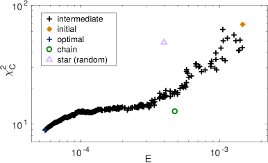
Figure 2: Correlation of the cost function $\chi^{2}_{C}$ and the Monte Carlo energy $E$ at intermediate steps of the optimization procedure (black crosses). $\chi^{2}_{C}$ measures the quality of the representation of the non-interacting full system by the 10-site cluster. In addition, we show the random starting point (orange star), the optimized representation (blue cross), the respective values of a chain representation cut after 10 sites (green circle) and an arbitrary selected 10-site star (cyan triangle).

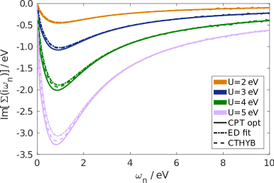
Figure 3: Matsubara self-energy of the optimized 10-site cluster (full lines) compared to the ED self-energy of a fitted 10-site system (dash-dotted lines) and a CTHYB result using the continuous bath DOS (dashed lines). The self-energy is shown for interaction values of $U=2,3,4\text{ and }$5\text{\,}\mathrm{eV}$$.

In Fig. 3 the self-energy $\Sigma(i\omega_{n})$ of the optimized system on the Matsubara axis is shown for different values of $U$. We compare it to results obtained at an inverse temperature of $\beta=$100\text{\,}\mathrm{eV}^{-1}$$ with the TRIQS/CTHYB solver [25], which is based on continuous-time quantum Monte Carlo in the hybridization expansion (CTHYB) [26; 27]. Additionally, we show the self-energies calculated with plain ED for a $L=10$ system. As the CPT self-energy of the full AIM is given by the self-energy of the 10-site cluster, we can only expect it to be compatible with CTHYB on a similar level as the ED self-energies are. For $U<=$4\text{\,}\mathrm{eV}$$ the ED self-energies are even slightly closer to the CTHYB result (see Fig. 3). Nevertheless, the important message conveyed by Figs. 2 and 3 is that the minimization of the off-diagonal block $T$ is a proper procedure to obtain a good representation of the full AIM system by the 10-site cluster.

The actual advantage of CPT is revealed on the level of the spectral function $A(\omega)$, which results from coupling the interacting cluster to the remainder of the non-interacting bath. In Fig. 4 we show the CPT spectral function (red) of the optimized system ($L=64$) for interaction values $U=0,1,2,\text{ and }$3\text{\,}\mathrm{eV}$$. We compare our results to spectral functions obtained with the density matrix renormalization group (DMRG) [28; 29] and real-time evolution (as in Ref. [30]) using matrix product states (MPS), colored in black. This approach is able to provide an excellent spectral resolution on the whole real-frequency axis [30; 31; 32]. We use the star representation of the $L=64$ AIM for the MPS calculation with a truncated weight of $10^{-10}$. Additionally, we show the results of the 10-site ED system (gray). In contrast to ED, which exhibits strong finite size effects, the CPT optimization scheme provides smoother spectral functions which are in much better agreement with the MPS results. This difference is particularly pronounced for the smaller $U$ values, which is a consequence of CPT becoming exact for $U\rightarrow 0$. Up to the influence of the discretization, CPT reproduces the non-interacting spectral function for $U=$0\text{\,}\mathrm{eV}$$ (see top grap in Fig. 4). Of course, for higher values of $U$ the energy resolution is limited by the size of the exactly solved system ($L_{C}$), which can be improved on by including more sites in the interacting cluster.

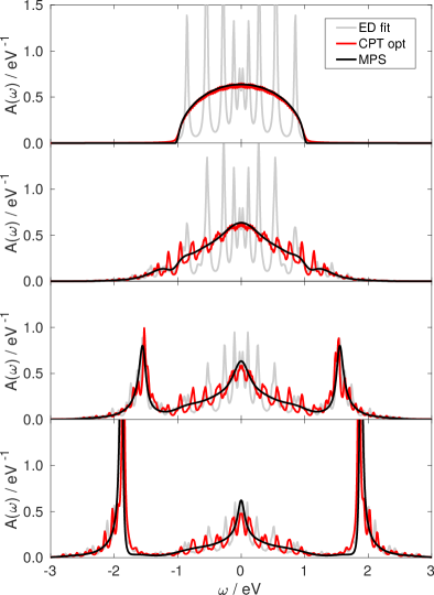
Figure 4: Spectral function $A(\omega)$ of the AIM with a particle-hole symmetric semi-circular bath DOS. The CPT interacting spectral functions $A(\omega)$ of the optimized system of size $L=64$ and $L_{C}=10$ (red) is compared to MPS results for the $L=64$ system in star representation (black) and to the ED result for a 10-site system (gray). A numerical broadening of $\eta=$0.02\text{\,}\mathrm{eV}$$ was used to calculate the ED and CPT spectral functions.

4 Conclusion

In this work we introduced a bath optimization scheme for the Anderson impurity model. Using unitary transformations in the bath degrees of freedom, we minimize the coupling between a small cluster containing the interacting impurity site and the remaining sites of the bath. These transformations leave the impurity DOS of the non-interacting bath invariant. In general, the proposed scheme can be useful for all CPT-based methods when parts of the entire system are non-interacting, but it does in principle also provide a guideline to construct finite-size representations of hybridization functions as needed, e.g., in the framework of dynamical mean-field theory. For a large enough number of bath sites, the initial AIM can be obtained directly on the real-frequency axis, and thus a fit on the Matsubara axis can be avoided. In this work we have presented a proof of concept, but anticipate to explore the bath optimization scheme for systems without particle-hole symmetry and multi-orbital impurity models.

References

References

- [1] P. W. Anderson, Localized Magnetic States in Metals, Phys. Rev. 124 (1961) 41–53. doi:10.1103/PhysRev.124.41.
- [2] M. Caffarel, W. Krauth, Exact diagonalization approach to correlated fermions in infinite dimensions: Mott transition and superconductivity, Phys. Rev. Lett. 72 (1994) 1545–1548. doi:10.1103/PhysRevLett.72.1545.
- [3] A. Georges, G. Kotliar, W. Krauth, M. J. Rozenberg, Dynamical mean-field theory of strongly correlated fermion systems and the limit of infinite dimensions, Rev. Mod. Phys. 68 (1996) 13–125. doi:10.1103/RevModPhys.68.13.
- [4] M. Capone, L. de’ Medici, A. Georges, Solving the dynamical mean-field theory at very low temperatures using the Lanczos exact diagonalization, Phys. Rev. B 76 (2007) 245116. doi:10.1103/PhysRevB.76.245116.
- [5] A. Liebsch, H. Ishida, Temperature and bath size in exact diagonalization dynamical mean field theory, J. Phys.: Condens. Matter 24 (5) (2012) 053201. doi:10.1088/0953-8984/24/5/053201.
- [6] D. Sénéchal, Bath optimization in the cellular dynamical mean-field theory, Phys. Rev. B 81 (2010) 235125. doi:10.1103/PhysRevB.81.235125.
- [7] M. Schüler, C. Renk, T. O. Wehling, Variational exact diagonalization method for Anderson impurity models, Phys. Rev. B 91 (2015) 235142. doi:10.1103/PhysRevB.91.235142.
- [8] M. Granath, H. U. R. Strand, Distributional exact diagonalization formalism for quantum impurity models, Phys. Rev. B 86 (2012) 115111. doi:10.1103/PhysRevB.86.115111.
- [9] D. Zgid, G. K.-L. Chan, Dynamical mean-field theory from a quantum chemical perspective, J. Chem. Phys. 134 (9) (2011) 094115. doi:10.1063/1.3556707.
- [10] D. Zgid, E. Gull, G. K.-L. Chan, Truncated configuration interaction expansions as solvers for correlated quantum impurity models and dynamical mean-field theory, Phys. Rev. B 86 (2012) 165128. doi:10.1103/PhysRevB.86.165128.
- [11] C. Lin, A. A. Demkov, Efficient variational approach to the impurity problem and its application to the dynamical mean-field theory, Phys. Rev. B 88 (2013) 035123. doi:10.1103/PhysRevB.88.035123.
- [12] Y. Lu, M. Höppner, O. Gunnarsson, M. W. Haverkort, Efficient real-frequency solver for dynamical mean-field theory, Phys. Rev. B 90 (2014) 085102. doi:10.1103/PhysRevB.90.085102.
-
[13]
A. Go, A. J. Millis,
Adaptively
truncated Hilbert space based impurity solver for dynamical mean-field
theory, Phys. Rev. B 96 (2017) 085139.
doi:10.1103/PhysRevB.96.085139.
URL https://link.aps.org/doi/10.1103/PhysRevB.96.085139 - [14] C. Gros, R. Valentí, Cluster expansion for the self-energy: A simple many-body method for interpreting the photoemission spectra of correlated Fermi systems, Phys. Rev. B 48 (1993) 418–425. doi:10.1103/PhysRevB.48.418.
- [15] D. Sénéchal, D. Perez, M. Pioro-Ladrière, Spectral Weight of the Hubbard Model through Cluster Perturbation Theory, Phys. Rev. Lett. 84 (2000) 522–525. doi:10.1103/PhysRevLett.84.522.
- [16] D. Sénéchal, D. Perez, D. Plouffe, Cluster perturbation theory for Hubbard models, Phys. Rev. B 66 (2002) 075129. doi:10.1103/PhysRevB.66.075129.
- [17] M. Potthoff, M. Aichhorn, C. Dahnken, Variational Cluster Approach to Correlated Electron Systems in Low Dimensions, Phys. Rev. Lett. 91 (2003) 206402. doi:10.1103/PhysRevLett.91.206402.
- [18] Potthoff, M., Self-energy-functional approach to systems of correlated electrons, Eur. Phys. J. B 32 (4) (2003) 429–436. doi:10.1140/epjb/e2003-00121-8.
- [19] Potthoff, M., Self-energy-functional approach: Analytical results and the Mott-Hubbard transition, Eur. Phys. J. B 36 (3) (2003) 335–348. doi:10.1140/epjb/e2003-00352-7.
- [20] M. Nuss, E. Arrigoni, M. Aichhorn, W. von der Linden, Variational cluster approach to the single-impurity Anderson model, Phys. Rev. B 85 (2012) 235107. doi:10.1103/PhysRevB.85.235107.
- [21] C. Weber, A. Amaricci, M. Capone, P. B. Littlewood, Augmented hybrid exact-diagonalization solver for dynamical mean field theory, Phys. Rev. B 86 (2012) 115136. doi:10.1103/PhysRevB.86.115136.
- [22] C. Lanczos, An iteration method for the solution of the eigenvalue problem of linear differential and integral operators, J. Res. Natl. Stand. 45 (1950) 255–282.
- [23] A. Ruhe, Implementation aspects of band Lanczos algorithms for computation of eigenvalues of large sparse symmetric matrices, Math. Comp. 33 (1979) 680–687. doi:10.1090/S0025-5718-1979-0521282-9.
- [24] J. C. Lagarias, J. A. Reeds, M. H. Wright, P. E. Wright, Convergence Properties of the Nelder–Mead Simplex Method in Low Dimensions, SIAM J. Optim. 9 (1) (1998) 112–147. doi:10.1137/S1052623496303470.
- [25] P. Seth, I. Krivenko, M. Ferrero, O. Parcollet, TRIQS/CTHYB: A continuous-time quantum Monte Carlo hybridisation expansion solver for quantum impurity problems, Comput. Phys. Commun. 200 (2016) 274 – 284. doi:10.1016/j.cpc.2015.10.023.
- [26] P. Werner, A. Comanac, L. de’ Medici, M. Troyer, A. J. Millis, Continuous-Time Solver for Quantum Impurity Models, Phys. Rev. Lett. 97 (2006) 076405. doi:10.1103/PhysRevLett.97.076405.
- [27] P. Werner, A. J. Millis, Hybridization expansion impurity solver: General formulation and application to Kondo lattice and two-orbital models, Phys. Rev. B 74 (2006) 155107. doi:10.1103/PhysRevB.74.155107.
- [28] S. R. White, Density matrix formulation for quantum renormalization groups, Phys. Rev. Lett. 69 (1992) 2863–2866. doi:10.1103/PhysRevLett.69.2863.
- [29] U. Schollwöck, The density-matrix renormalization group in the age of matrix product states, Ann. Phys. 326 (2011) 96–192. doi:10.1016/j.aop.2010.09.012.
- [30] D. Bauernfeind, M. Zingl, R. Triebl, M. Aichhorn, H. G. Evertz, Fork Tensor-Product States: Efficient Multiorbital Real-Time DMFT Solver, Phys. Rev. X 7 (2017) 031013. doi:10.1103/PhysRevX.7.031013.
- [31] F. A. Wolf, I. P. McCulloch, U. Schollwöck, Solving nonequilibrium dynamical mean-field theory using matrix product states, Phys. Rev. B 90 (2014) 235131. doi:10.1103/PhysRevB.90.235131.
- [32] M. Ganahl, M. Aichhorn, H. G. Evertz, P. Thunström, K. Held, F. Verstraete, Efficient DMFT impurity solver using real-time dynamics with matrix product states, Phys. Rev. B 92 (2015) 155132. doi:10.1103/PhysRevB.92.155132.
- [33] O. Parcollet, M. Ferrero, T. Ayral, H. Hafermann, I. Krivenko, L. Messio, P. Seth, TRIQS: A toolbox for research on interacting quantum systems, Comput. Phys. Commun. 196 (2015) 398 – 415. doi:10.1016/j.cpc.2015.04.023.
- [34] ITensor library, http://itensor.org/.