Time irreversibility and multifractality of power along single particle trajectories in turbulence

Abstract

The irreversible turbulent energy cascade epitomizes strongly non-equilibrium systems. At the level of single fluid particles, time irreversibility is revealed by the asymmetry of the rate of kinetic energy change, the Lagrangian power, whose moments display a power-law dependence on the Reynolds number, as recently shown by Xu et al. [H Xu et al, Proc. Natl. Acad. Sci. U.S.A. 111, 7558 (2014)]. Here Lagrangian power statistics are rationalized within the multifractal model of turbulence, whose predictions are shown to agree with numerical and empirical data. Multifractal predictions are also tested, for very large Reynolds numbers, in dynamical models of the turbulent cascade, obtaining remarkably good agreement for statistical quantities insensitive to the asymmetry and, remarkably, deviations for those probing the asymmetry. These findings raise fundamental questions concerning time irreversibility in the infinite-Reynolds-number limit of the Navier-Stokes equations.

I Introduction

In nature, the majority of the processes involving energy flow occur in nonequilibrium conditions from the molecular scale of biology Ritort (2008) to astrophysics Priest (2014). Understanding such nonequilibrium processes is of great interest at both fundamental and applied levels, from small-scale technology Blickle and Bechinger (2012) to climate dynamics Kleidon (2010). A key aspect of nonequilibrium systems is the behavior of fluctuations that markedly differ from equilibrium ones. As for the latter, detailed balance establishes equiprobability of forward and backward transitions between any two states, a statistical manifestation of time reversibility Onsager (1931), while, irreversibility of nonequilibrium processes breaks detailed balance. In three-dimensional (3D) turbulence, a prototype of very far-from-equilibrium systems, detailed balance breaks in a fundamental way Rose and Sulem (1978): It is more probable to transfer energy from large to small scales than its reverse. Indeed, in statistically stationary turbulence, energy, supplied at scale $L$ at rate $\epsilon$ ($\approx U_{L}^{3}/L$, $U_{L}$ being the root mean square single-point velocity), is transferred with a constant flux approximately equal to $\epsilon$ up to the scale $\eta$, where it is dissipated at the same rate $\epsilon$, even for vanishing viscosity ($\nu\to 0$) Frisch (1995). As a result, time reversibility, formally broken by the viscous term, is not restored for $\nu\to 0$ Falkovich and Sreenivasan (2006). Time irreversibility is unveiled by the asymmetry of two-point statistical observables. In particular, the constancy of the energy flux directly implies, in the Eulerian frame, a non vanishing third moment of longitudinal velocity difference between two points at distance $r$ (the $\frac{4}{5}$ law Frisch (1995)) and, in the Lagrangian frame, a faster separation of particle pairs backward than forward in time Falkovich and Frishman (2013); Jucha et al. (2014).

Remarkably, time irreversibility has been recently discovered at the level of single-particle statistics Xu et al. (2014); Pumir et al. (2014) that is not a priori sensitive to the existence of a nonzero energy flux. This opens important challenges also at applied levels for stochastic modelization of single-particle transport, e.g., in turbulent environmental flows Wilson and Sawford (1996). Both experimental and numerical data revealed that the temporal dynamics of Lagrangian kinetic energy $E(t)=\frac{1}{2}v^{2}(t)$, where $\bm{v}(t)=\bm{u}(\bm{x}(t),t)$ is the Lagrangian velocity along a particle trajectory $\bm{x}(t)$, is characterized by events where $E(t)$ grows slower than it decreases. Such flight-crash events result in the asymmetry of distribution of the Lagrangian power, $p(t)=\dot{E}=\bm{v}(t)\cdot\bm{a}(t)$ ($\bm{a}\equiv\dot{\bm{v}}=\partial_{t}\bm{u}+\bm{u}\cdot\bm{\nabla}\bm{u}$ being the fluid particle acceleration). While in stationary conditions the mean power vanishes $\langle p\rangle=0$, the third moment is increasingly negative with the Taylor scale Reynolds number $\mathrm{Re}_{\lambda}\approx(U_{L}L/\nu)^{1/2}\approx T_{L}/\tau_{\eta}$ measuring the ratio between the timescales of energy injection $T_{L}$ and dissipation $\tau_{\eta}$, which easily exceeds $10^{3}$ in the laboratory. In particular, it was found that $\langle p^{3}\rangle/\epsilon^{3}\sim-\mathrm{Re}_{\lambda}^{2}$ Xu et al. (2014); Pumir et al. (2014) and $\langle p^{2}\rangle/\epsilon^{2}\sim\mathrm{Re}_{\lambda}^{4/3}$. Interestingly, the $\mathrm{Re}_{\lambda}$ dependence deviates from the dimensional prediction based on Kolmogorov phenomenology Frisch (1995) $\langle p^{q}\rangle/\epsilon^{q}\propto\mathrm{Re}_{\lambda}^{q/2}$, signaling that the Lagrangian power is strongly intermittent as exemplified by its spatial distribution and the strong non-Gaussian tails of the probability distribution function of $p$ (Fig. 1).

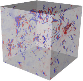
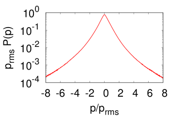
Figure 1: Shown on the left is a three-dimensional rendering of the Lagrangian power spatial distribution in the whole simulation volume. Red (blue) represents the isosurfaces $p=\pm 6p_{rms}$ ($p_{rms}=\langle p^{2}\rangle^{1/2}$), which appear clusterized in dipole structures. Shown on the right is the log-lin standardized PDF of $p$ for $\mathrm{Re}_{\lambda}\approx 104$. Notice that the asymmetry of the distribution is very small, hence the difficulty to quantify and rationalize the physics behind irreversible effects along a particle trajectory.

From a theoretical point of view, the above scaling behavior of the power with $\mathrm{Re}_{\lambda}$ implies that the skewness of the probability density function (PDF) of $p$, $S=\langle p^{3}\rangle/\langle p^{2}\rangle^{3/2}\,,$ is constant, suggesting that time irreversibility is robust and persists even in the limit $\mathrm{Re}_{\lambda}\to\infty$. It is important to stress that one might use different dimensionless measures of the symmetry breaking, e.g., $\tilde{S}=\langle p^{3}\rangle/\langle|p|^{3}\rangle\,,$ which directly probes the ratio between the symmetric and asymmetric contributions to the PDF. In the presence of anomalous scaling $S$ and $\tilde{S}$ can have a different $\mathrm{Re}_{\lambda}$ dependence, as highlighted for the problem of statistical recovery of isotropy Biferale and Vergassola (2001).

The aim of our work is twofold. First, we use direct numerical simulations (DNSs) of 3D Navier-Stokes equations (NSEs) to quantify the degree of recovery of time reversibility along single-particle trajectories using different definitions as discussed above. Second, we show that it is possible to extend the multifractal formalism (MF) Frisch and Parisi (1985) to predict the scaling of the absolute value of the Lagrangian power statistics. Moreover, in order to explore a wider range of Reynolds numbers, we also investigate the equivalent of the Lagrangian power statistics in shell models Biferale (2003); Bohr et al. (2005).

The rest of the paper is organized as follows. Section II is devoted to a brief review of the multifractal formalism for fully developed turbulence and the predictions for the statistics of the Lagrangian power. In Sec. III we compare these predictions with the results obtained from direct numerical simulations of the Navier-Stokes equations and from a shell model of turbulence. Section IV is devoted to a summary and conclusions. The Appendix reports some details of the numerical simulations.

II Theoretical predictions by the multifractal model

We start by recalling the MF for the Eulerian statistics Frisch and Parisi (1985); Frisch (1995). The basic idea is to replace the global scale invariance in the manner of Kolmogorov with a local scale invariance, by assuming that spatial velocity increments $\delta_{r}u$ over a distance $r\ll L$ are characterized by a range of scaling exponents $h\in\mathcal{I}\equiv(h_{m},h_{M})$, i.e., $\delta_{r}u\sim u_{L}(r/L)^{h}$. Eulerian structure functions $\langle(\delta_{r}u)^{q}\rangle$ are obtained by integrating over $h\in\mathcal{I}$ and the large-scale velocity $u_{L}$ statistics $\mathcal{P}(u_{L})$, which can be assumed to be independent of $h$. The MF assumes the exponent $h$ to be realized on a fractal set of dimension $D(h)$, so the probability to observe a particular value of $h$, for $r\ll L$, is $\mathcal{P}_{h}(r)\sim(r/L)^{3-D(h)}$. Hence, we find $\langle(\delta_{r}u)^{q}\rangle\sim\langle u_{L}^{q}\rangle\int_{h\in\mathcal{I}}dh(r/L)^{hq+3-D(h)}\sim\langle u_{L}^{q}\rangle(r/L)^{\zeta_{q}}$, where a saddle-point approximation for $r\ll L$ gives

$$\zeta_{q}=\inf_{h\in\mathcal{I}}\{hq+3-D(h)\}\,.$$ (1)

For the MF to be predictive, $D(h)$ should be derived from the NSE, which is out of reach. One can, however, use the measured exponents $\zeta_{p}$ and, by inverting (1), derive an empirical $D(h)$. Here, following She and Leveque (1994), we use

$$D(h)=3-d_{0}-d(h)\left[\ln\left({d(h)}/{d_{0}}\right)-1\right]\,,$$ (2)

with $d(h)={3(1/9-h)}/{\ln\beta}$ and $d_{0}={2}/{[3(1-\beta)]}$ corresponding, via (1), to $\zeta_{q}=q/9+(2/3)(1-\beta^{q/3})/(1-\beta)$, which, for $\beta=0.6$, fits measured exponents fairly well Arnéodo et al. (2008).

The MF has been extended from Eulerian to Lagrangian velocity increments Borgas (1993); Boffetta et al. (2002). The idea is that temporal velocity differences $\delta_{\tau}v$ over a time lag $\tau$, along fluid particle trajectories, can be connected to equal time spatial velocity differences $\delta_{r}u$ by assuming that the largest contribution to $\delta_{\tau}v$ comes from eddies at a scale $r$ such that $\tau\sim r/\delta_{r}u$. This implies $\delta_{\tau}v\sim\delta_{r}u$, with

$$\tau\sim T_{L}({r}/{L})^{1-h}\,,$$ (3)

where $T_{L}=L/u_{L}$. By combining Eq. (3) and the $D(h)$ obtained from Eulerian statistics, one can derive a prediction for Lagrangian structure functions, which has been found to agree with experimental and DNS data Boffetta et al. (2002); Chevillard et al. (2003); Biferale et al. (2004); Arnéodo et al. (2008). The MF can be used also for describing the statistics of the acceleration $a$ along fluid elements Borgas (1993); Biferale et al. (2004). The acceleration can be estimated by assuming

$$a\sim{\delta_{\tau_{\eta}}v}/{\tau_{\eta}}\,.$$ (4)

According to the MF, the dissipative scale fluctuates as $\eta\sim(\nu L^{h}/u_{L})^{1/(1+h)}$ Frisch and Vergassola (1991), which leads, via (3), to

$$\tau_{\eta}\sim T(\nu/Lu_{L})^{(1-h)/(1+h)}\,.$$ (5)

Substituting (5) in (4) yields the acceleration conditioned on given values of $h$ and $u_{L}$:

$$a\sim\nu^{(2h-1)/(1+h)}u_{L}^{3/(1+h)}L^{-3h/(1+h)}\,.$$ (6)

Equation (6) has been successfully used to predict the acceleration variance Borgas (1993) and PDF Biferale et al. (2004).

We now use (6) to predict the scaling behavior of the Lagrangian power moments with $\mathrm{Re}_{\lambda}$. These can be estimated as $\langle p^{q}\rangle\!\sim\!\langle(au_{L})^{q}\rangle\!\!\sim\!\!\int du_{L}\mathcal{P}(u_{L})\int_{h\in\mathcal{I}}dh\mathcal{P}_{h}(\tau_{\eta})(au_{L})^{q}$ with $\mathcal{P}_{h}(\tau_{\eta})=(\tau_{\eta}/T)^{{[3-D(h)]}/{(1-h)}}$. Using (5) with $\nu=U_{L}L\mathrm{Re}_{\lambda}^{2}$ (with $U_{L}^{2}=\langle u_{L}^{2}\rangle$), we have

$$\frac{\langle p^{q}\rangle}{\epsilon^{q}}\!\sim\!\!\int\!\!d\tilde{v}\mathcal{P}(\tilde{v})\!\!\int_{h\in\mathcal{I}}\!\!\!\!\!\!\!dh\tilde{v}^{[4q+h-3+D(h)]/(1+h)}\!\mathrm{Re}_{\lambda}^{2[(1-2h)q-3+D(h)]/(1+h)}\,,$$ (7)

with $\tilde{v}=u_{L}/U_{L}$ . In the limit $\mathrm{Re}_{\lambda}\to\infty$, a saddle point approximation of the integral (7) yields, up to a multiplicative constant (depending on the large scale statistics), $\langle p^{q}\rangle/\epsilon^{q}\!\!\sim\mathrm{Re}_{\lambda}^{\alpha(q)}$ with

$$\alpha(q)=\sup_{h}\left\{2\frac{(1-2h)q-3+D(h)}{1+h}\right\}\,.$$ (8)

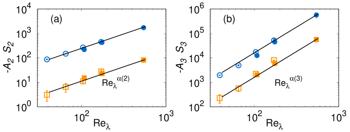
Figure 2: Scaling behavior of Lagrangian power moments (9) $\mathcal{S}_{q}$ (blue circles) and $-\mathcal{A}_{q}$ (orange squares) for (a) $q=2$ and (b) $q=3$. Data refer to DNS1 (closed symbols) and DNS2 (open symbols) datasets, described in the Appendix. Solid lines show the slopes (a) $\alpha(2)=1.17$ and (b) $\alpha(3)=2.1$ predicted by the MF via (8) with (2) for $\beta=0.6$. Errors bars have been obtained as standard errors over independent configurations of the turbulent field. We used from 5 to 40 configurations spaced by approximately $T_{L}$, depending on the resolution.

III Comparison with numerical simulations

To test the MF predictions (8) we use two sets of DNS of homogeneous isotropic turbulence on cubic lattices of sizes from $128^{3}$ up to $2048^{3}$, with $\mathrm{Re}_{\lambda}$ up to $540$, obtained with two different forcings (see the Appendix for details). In particular, to probe both the symmetric and asymmetric components of the Lagrangian power statistics, we study the nondimensional moments

$$\mathcal{S}_{q}=\langle|p|^{q}\rangle/\epsilon^{q},\quad\mathcal{A}_{q}=\langle p|p|^{q-1}\rangle/\epsilon^{q}\,,$$ (9)

where the latter vanishes for a symmetric (time-reversible) PDF. In Fig. 2 we show the second-and third-order moments of (9) as a function of $\mathrm{Re}_{\lambda}$. We observe that (i) the MF prediction (8) is in excellent agreement with the scaling of $\mathcal{S}_{q}$ (see also Fig. 3) and (ii) the asymmetry probing moments $\mathcal{A}_{q}$ are negative, confirming the existence of the time-symmetry breaking, and scale with exponents compatible with those of $\mathcal{S}_{q}$. This implies that time reversibility is not recovered even for $\mathrm{Re}_{\lambda}\to\infty$. Actually, irreversibility is independent of $\mathrm{Re}_{\lambda}$ if measured in terms of the homogeneous asymmetry ratio $\tilde{S}=\mathcal{A}_{q}/\mathcal{S}_{q}$, while if quantified in terms of the standard skewness $S$, it grows as $\mathrm{Re}_{\lambda}^{\chi}$ with $\chi=\alpha(3)-(3/2)\alpha(2)\simeq 0.35$ due to anomalous scaling. In the inset of Fig. 3 we compare $S$ with $\tilde{S}$. Evaluating (8) with $D(h)$ given by (2), we obtain $\alpha(2)\approx 1.17$ and $\alpha(3)\approx 2.10$, which are close to the $4/3$ and $2$ reported in Xu et al. (2014). We remark that the authors of Xu et al. (2014) explained the observed exponents by assuming that the dominating events are those for which the particle travels a distance $r\sim U_{L}\tau$ in a frozenlike turbulent velocity field, so that $\delta_{\tau_{\eta}}v\sim(\epsilon\tau_{\eta}U_{L})^{{1}/{3}}$. Hence, for the acceleration (4) one has $a\sim U_{L}^{{1}/{3}}\epsilon^{{1}/{3}}\tau_{\eta}^{-{2}/{3}}$, which, using the dimensional prediction $\tau_{\eta}=(\nu/\epsilon)^{{1}/{2}}$, ends up in $p\sim U_{L}a\sim U_{L}^{{4}/{3}}\epsilon^{{2}/{3}}\nu^{-{1}/{3}}\sim\epsilon\mathrm{Re}_{\lambda}^{2/3}$. This argument provides only a linear approximation $2q/3$ for $\alpha(q)$, while the multifractal model is able to describe its nonlinear dependence on $q$. In Fig. 3 we show the whole set of exponents for both $\mathcal{A}_{q}$ and $\mathcal{S}_{q}$ as observed in DNS data and compare them with the prediction (8).

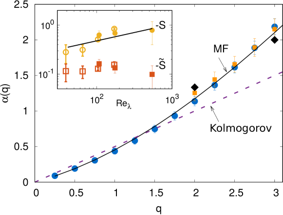
Figure 3: Scaling exponents of Lagrangian power moments $\alpha(q)$ from DNS data, obtained by fitting $\mathcal{S}_{q}$ (blue circles) and $-\mathcal{A}_{q}$ (orange squares) as power of $\mathrm{Re}_{\lambda}$. Error bars have been obtained by varying the fitting region; when they are not visible it is because they are of the order of or smaller than the symbol size. Notice that $\mathcal{A}_{q}$ is positive for $q<1$, zero for $q=1$ (by stationarity) and negative for $q>1$. We only show exponents for $q\geq 2$ because for $1<q<2$ insufficient statistics leads to a poor scaling behavior. Solid and dashed curves correspond to the MF (8) and Kolmogorov [$\alpha(q)=q/2$] dimensional prediction, respectively. Black diamonds show the exponents found in Xu et al. (2014). The inset shows the nondimensional measure of the asymmetry in terms of the skewness $S=\langle p^{3}\rangle/\langle p^{2}\rangle^{3/2}$ (yellow circles) and of the statistically homogeneous asymmetry ratio $\tilde{S}=\langle p^{3}\rangle/\langle|p|^{3}\rangle$ (red squares). The solid line shows the slope $\alpha(3)-(3/2)\alpha(2)\simeq 0.35$ predicted by the MF (see the text). open and closed symbols are as in Fig. 2.

It is worth noticing that the MF provides an excellent prediction for the statistics of $p$ also in 1D compressible turbulence, i.e., in the Burgers equation, studied in Grafke et al. (2015). Here, out of a smooth ($h=1$) velocity field, the statistically dominant structures are shocks ($h=0$). The velocity statistics is thus bifractal with $D(1)=1$ and $D(0)=0$ Bec and Khanin (2007). Adapting (8) to one dimension and noticing that $\mathrm{Re}\propto\mathrm{Re}_{\lambda}^{2}$, we have $\langle p^{q}\rangle\sim\mathrm{Re}^{\alpha_{1D}(q)}$ with $\alpha_{1D}(q)=\sup_{h}\{[(1-2h)q-1+D(h)]/(1+h)\}$, which for Burgers means $\alpha_{1D}(q)=q-1$, in agreement with the results of Grafke et al. (2015).

To further investigate the scaling behavior of the symmetric and asymmetric components of the power statistics in a wider range of Reynolds numbers and with higher statistics, in the following we study Lagrangian power within the framework of shell models of turbulence Biferale (2003); Bohr et al. (2005). Shell models are dynamical systems built to reproduce the basic phenomenology of the energy cascade on a discrete set of scales, $r_{n}=k_{n}^{-1}=L2^{-n}$ ($n=0,\ldots,N$), which allow us to reach high Reynolds numbers. For each scale $r_{n}$, the velocity fluctuation is represented by a single complex variable $u_{n}$, which evolves according to the differential equation L’vov et al. (1998)

$$\dot{u}_{n}=ik_{n}(u_{n+2}u^{*}_{n+1}-\frac{1}{4}u_{n+1}u^{*}_{n-1}+\frac{1}{8}u_{n-1}u_{n-2})-\nu k_{n}^{2}u_{n}+f_{n}$$ (10)

whose structure is a cartoon of the 3D NSE in Fourier space but for the nonlinear term that restricts the interactions to neighboring shells, as justified by the idea localness of the energy cascade Rose and Sulem (1978). Energy is injected with rate $\epsilon=\langle\sum_{n}\mathrm{Re}\{f_{n}u_{n}^{*}\}\rangle$. See the Appendix for details on forcing and simulations. As shown in L’vov et al. (1998), this model displays anomalous scaling for the velocity structure functions, $\langle|u_{n}|^{q}\rangle\sim k_{n}^{-\zeta_{q}}$, with exponents remarkably close to those observed in turbulence and in very good agreement with the MF prediction (1).

Following Boffetta et al. (2002), we model the Lagrangian velocity along a fluid particle as the sum of the real part of velocity fluctuations at all shells $v(t)\equiv\sum_{n=1}^{N}\mathrm{Re}\{u_{n}\}$. Analogously, we define the Lagrangian acceleration $a\equiv\sum_{n=1}^{N}\mathrm{Re}\{\dot{u}_{n}\}$ and power $p(t)=v(t)a(t)$.

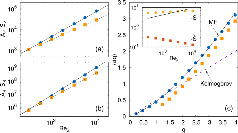
Figure 4: Lagrangian power statistics in the shell model with $N=30$ shells at varying $\nu$. $\mathrm{Re}_{\lambda}$-dependence of $\mathcal{S}_{q}$ and $-\mathcal{A}_{q}$ is shown for (a) $q=2$ and (b) $q=3$ compared with the MF prediction (8) (solid lines) and the best fit of the asymmetry-sensitive observables (dashed lines) providing slopes (a) $0.93(1)$ and (b) $1.87(1)$. Notice that $-\mathcal{A}_{q}$ is shifted upward to highlight the different scaling behavior. (c) Scaling exponents $\alpha(q)$ obtained by fitting $\mathcal{S}_{q}$ (blue circles) and $-\mathcal{A}_{q}$ (orange squares) as power laws in $\mathrm{Re}_{\lambda}$, compared with (black solid curve) the MF prediction (8) and (purple dashed curve) Kolmogorov dimensional scaling. Errors on the fitted values have been obtained by varying the fitting region; they are of the order of or smaller than the symbol size. The inset shows the nondimensional measure of the asymmetry in terms of the skewness $S=\langle p^{3}\rangle/\langle p^{2}\rangle^{3/2}$ (yellow circles) and of the statistically homogeneous asymmetry ratio $\tilde{S}=\langle p^{3}\rangle/\langle|p|^{3}\rangle$ (red squares). Notice that the different scaling behavior of $\mathcal{S}_{q}$ and $-\mathcal{A}_{q}$ reflects on the $\mathrm{Re}_{\lambda}$ dependence of the $S$ that deviates from the MF slope $\alpha(3)-(3/2)\alpha(2)$ (solid line). Data in (a), (b) and the inset in (c) have been obtained by averaging over ten realizations, each lasting $10^{6}\,T_{L}$; the standard error over the ten realization is of the order of or smaller than the symbol size.

In Figs. 4(a) and 4(b) we show the moments $\mathcal{S}_{q}$ and $\mathcal{A}_{q}$ for $q=2,3$ obtained from the shell model. The symmetric ones $\mathcal{S}_{q}$ perfectly agree with the multifractal prediction obtained using the same $D(h)$, i.e., (2) for $\beta=0.6$, which fits the Eulerian statistics. The asymmetry-sensitive moments $\mathcal{A}_{q}$ are negative (for $q>1$), as in Navier-Stokes turbulence, and display a power-law dependence on $\mathrm{Re}_{\lambda}$ with a different scaling respect to their symmetric analogs. In particular, as summarized in Fig. 4(c), we observe smaller exponents with respect to the MF up to $q=4$. Rephrased in terms of the skewness, these findings mean that the time asymmetry becomes weaker and weaker with increasing Reynolds numbers if measured in terms of $\tilde{S}$ [Fig. 4(c) inset], as distinct from what was observed for the NSE (Fig. 3 inset). The standard skewness $S$, on the other hand, is still an increasing function of $\mathrm{Re}_{\lambda}$ though with an exponent smaller than the MF prediction $\alpha(3)-(3/2)\alpha(2)$, because $\mathcal{A}_{3}$ has a shallower slope than the multifractal one.

IV Conclusions

We have shown that the multifractal formalism predicts the scaling behavior of the Lagrangian power moments in excellent agreement with DNS data and with previous results on the Burgers equation. In the range of explored $\mathrm{Re}_{\lambda}$, we have found that symmetric and antisymmetric moments share the same scaling exponents, and therefore the MF is able to reproduce both statistics. It is worth stressing that the effectiveness of the MF in describing the scaling of $\mathcal{A}_{q}$ is not obvious as the MF, in principle, bears no information on statistical asymmetries . By analyzing the Lagrangian power statistics in a shell model of turbulence, at Reynolds numbers much higher than those achievable in DNS, we found that symmetric and antisymmetric moments possess two different sets of exponents. While the former are still well described by the MF formalism, the latter, in the range of $q$ explored, are smaller. As a consequence, the ratios $\mathcal{A}_{q}/\mathcal{S}_{q}$ in the shell model decrease with $\mathrm{Re}_{\lambda}$. However, we observe that the mismatch between the two sets of scaling is compatible with the assumption that $\mathcal{A}_{q}\sim\mathcal{S}_{q}\langle\mathrm{sign}(p)\rangle$, i.e., that the main effect is given by a cancellation exponent introduced by the scaling of $\mathrm{sgn}(p)$. Our findings raise the question whether the apparent similar scaling among symmetric and asymmetric components in the NSE is robust for large Reynolds numbers or a sort of recovery of time symmetry would be observed also in Navier-Stokes turbulence as for shell models.

We conclude by mentioning another interesting open question. In Xu et al. (2014); Pumir et al. (2014) it was found that the Lagrangian power statistics is asymmetric also in statistically stationary 2D turbulence in the presence of an inverse cascade. Like in three dimensions, the third moment is negative and its magnitude grows with the separation between the timescale of dissipation by friction (at large scale) and of energy injection (at small scale), which is a measure of $\mathrm{Re}_{\lambda}$ for the inverse cascade range. Moreover, the scaling exponents are quantitatively close to the 3D ones. This raises the question on the origin of the scaling in 2two dimensions that cannot be rationalized within the MF, since the inverse cascade is not intermittent Boffetta and Ecke (2012). Likely, to answer the question one needs a better understanding of the influence of the physics at and below the forcing scale on the 2D Lagrangian power.

*

Appendix A Details on the numerical simulations

A.1 Direct Numerical Simulations

We performed two sets of DNSs at different resolutions and Reynolds numbers with two different forcing schemes. The values of the parameters characterizing all the simulations are shown in Table 1. In all cases we integrated the Navier-Stokes equations

$$\partial_{t}{\bm{u}}+{\bm{u}}\cdot{\bm{\nabla}}{\bm{u}}\equiv{\bm{a}}=-\bm{\bm{\nabla}}P+\nu\Delta{\bm{u}}+{\bm{f}}\;,$$ (11)

for the incompressible velocity field ${\bm{u}}({\bm{x}},t)$ with a fully parallel pseudo-spectral code, fully dealiased with $2/3$ rule Orszag (1971), in a cubic box of size $\mathcal{L}=2\pi$ with periodic boundary conditions. In (11) $P$ represents the pressure and $\nu$ is the kinematic viscosity of the fluid.

For the set of runs DNS1 we used a Sawford-type stochastic forcing, involving the solution of the stochastic differential equations Sawford (1991)

$$\begin{cases}d\tilde{f}_{i}=\tilde{a}_{i}(t)dt\,,\\ d\tilde{a}_{i}=-a_{1}\tilde{a}_{i}(t)dt-a_{2}\tilde{f}_{i}(t)dt+a_{3}dW_{i}(t)\,,\end{cases}$$ (12)

where $a_{1}=1/\tau_{f}$, $a_{2}=(1/8)/\tau_{f}^{2}$, $a_{3}=\sqrt{2a_{1}a_{2}}$, and $dW_{i}(t)=r\sqrt{dt}$ is an increment of a Wiener process ($r$ is a random Gaussian number with $\langle r\rangle=0$ and $\langle r^{2}\rangle=1$). The forcing $\bm{f}(\bm{k},t)$ in Fourier space is then

$$\bm{f}(\bm{k},t)=\begin{cases}i\bm{k}\times[i\bm{k}\times(0.16\,k^{-4/3}\tilde{\bm{f}})]\quad&\text{for}\quad k\in[k_{f,\mathrm{min}},k_{f,\mathrm{max}}]\\ 0\quad&\text{for}\quad k\notin[k_{f,\mathrm{min}},k_{f,\mathrm{max}}]\,.\end{cases}$$ (13)

Time integration is performed by a second-order Adams-Basforth scheme with exact integration of the linear dissipative term Canuto and Quarteroni (2006).

$\mathrm{Set}$	$N$	$\mathrm{Re}_{\lambda}$	$\epsilon$	$U$	$L$	$T_{L}$	$\eta$	$\tau_{\eta}$	$T$	$k_{f,\mathrm{min}}$	$k_{f,\mathrm{max}}$	$\tau_{f}$
DNS1	$2048$	$544$	$1.43$	$1.62$	$4.51$	$2.77$	$0.0021$	$0.015$	$15$	$0.5$	$1$	$0.14$
DNS1	$512$	$176$	$1.68$	$1.74$	$4.70$	$2.70$	$0.0083$	$0.035$	$10$	$0.5$	$1$	$0.6$
DNS1	$256$	$115$	$1.19$	$1.50$	$4.26$	$2.84$	$0.019$	$0.066$	$48$	$0.5$	$1$	$0.6$
DNS2	$1024$	$171$	$0.1$	$0.529$	$2.22$	$4.19$	$0.005$	$0.063$	$27$	$0$	$1.5$	n/a
DNS2	$512$	$104$	$0.1$	$0.520$	$2.11$	$4.06$	$0.01$	$0.10$	$96$	$0$	$1.5$	n/a
DNS2	$256$	$65$	$0.1$	$0.513$	$2.05$	$3.98$	$0.02$	$0.16$	$165$	$0$	$1.5$	n/a
DNS2	$128$	$38.9$	$0.1$	$0.507$	$1.95$	$3.85$	$0.04$	$0.25$	$165$	$0$	$1.5$	n/a

Table 1: Type of forcing, resolution $N$, Reynolds number $\mathrm{Re}_{\lambda}=U\lambda/\nu$ [$\lambda=(5E/Z)^{1/2}$ is the Taylor microscale, $\epsilon$ the mean energy dissipation rate, $E$ the kinetic energy, and $Z$ the enstrophy], large-scale velocity $U=(2E/3)^{1/2}$, integral scale $L=UE/\varepsilon$, integral time $T_{L}=E/\varepsilon$, dissipative scale $\eta=(\nu^{3}/\varepsilon)^{1/4}$, Kolmogorov time $\tau_{\eta}=(\nu/\varepsilon)^{1/2}$, total time of integration $T$, and correlation time used in the forcing of DNS1 $\tau_{f}$ [see Eq. (12)]. Because of the different forcing in the two sets of simulations, for DNS2 the contribution of the modes at wave numbers $k\leq 1$ have been removed in the analysis.

For the set of runs DNS2 we use a deterministic forcing acting on a spherical shell of wavenumbers in Fourier space $0<|{\bf k}|\leq k_{f}$, where $k_{f}=1.5$ with imposed energy input rate $\varepsilon$ Lamorgese et al. (2005). In Fourier space the forcing reads

$$\bm{f}(\bm{k},t)=\begin{cases}\varepsilon\bm{u}({\bf k},t)/[2E_{f}(t)]\quad&\text{for}\quad k\in[k_{f,\mathrm{min}},k_{f,\mathrm{max}}]\\ 0\quad&\text{for}\quad k\notin[k_{f,\mathrm{min}},k_{f,\mathrm{max}}]\,.\end{cases}$$ (14)

where $E_{f}(t)=\sum_{k=0}^{k_{f}}E(k,t)$, and $E(k,t)$ is the energy spectrum at time $t$. This forcing guarantees the constancy of the energy injection rate. Notice that Eq. (14) explicitly breaks the time-reversal symmetry; however, owing to the universality properties of turbulence with respect to the forcing, we expect this effect to be negligible as compared to the energy cascade. Time integration is performed by a second-order Runge-Kutta midpoint method with exact integration of the linear dissipative term Canuto and Quarteroni (2006); Boyd (2001). Simulations have a resolution $N$ sufficient to resolve the dissipative scale with $k_{\mathrm{max}}\eta\simeq 1.7$ ($k_{\mathrm{max}}=N/3$). We have checked in the simulations that the velocity field is statistically isotropic with a probability density function (for each component) close to a Gaussian.

Simulations are performed for several large-scale eddy turnover times $T$, after an initial transient to reach the turbulent state, in order to generate independent velocity fields in stationary conditions. From the velocity fields the acceleration field is then computed by evaluating the right hand side of (11) and the power field is obtained as $p={\bm{u}}\cdot{\bm{a}}$.

A.2 Simulations of the shell model

As for the shell model (10), simulations have been performed by fixing the number of shells $N=30$ and varying the viscosity $\nu$ in the range $[3.16\times 10^{-4},3.16\times 10^{-8}]$. For each value of $\nu$ we performed ten independent realizations lasting approximately $10^{6}T_{L}$ each. Time integration is performed using a fourth-order Runge-Kutta scheme with exact integration of the linear term. Forcing is stochastic and acts only on the first shell $f_{n}=f\delta_{n,1}$. The stochastic forcing is obtained by choosing $f=F(f^{R}+if^{I})$ with $F=1$ and

$$\dot{f}^{\alpha} = -\frac{1}{\tau_{f}}f^{\alpha}+\frac{\sqrt{2}}{\tau_{f}}\theta^{\alpha}(t)\,,$$ (15)

$$\dot{\theta}^{\alpha} = -\frac{1}{\tau_{f}}{\theta^{\alpha}}+\sqrt{\frac{2}{\tau_{f}}}\eta^{\alpha}(t)\,,$$ (16)

where $\eta^{\alpha}$ is a zero mean Gaussian variable with correlation $\langle\eta^{\alpha}(t)\eta^{\beta}(t^{\prime})\rangle=\delta_{\alpha\beta}\delta(t-t^{\prime})$. As a result, $f^{\alpha}$ is a zero mean Gaussian variable with correlation $\langle f^{\alpha}(t)f^{\beta}(t^{\prime})\rangle=\delta_{\alpha\beta}\frac{1}{\tau_{f}}\exp(-|t-t^{\prime}|/\tau_{f})(|t-t^{\prime}|+\tau_{f})$. In particular, we used $\tau_{f}=1$, which is of the order of the large-eddy turnover time $T_{L}$. Using a constant amplitude forcing, we obtained, within error bars, indistinguishable exponents (not shown).

References

- Ritort (2008) F. Ritort, “Nonequilibrium fluctuations in small systems: From physics to biology,” Adv. Chem. Phys. 137, 31 (2008).
- Priest (2014) E. Priest, Magnetohydrodynamics of the Sun (Cambridge University Press, Cambridge, 2014).
- Blickle and Bechinger (2012) V. Blickle and C. Bechinger, “Realization of a micrometre-sized stochastic heat engine,” Nature Phys. 8, 143 (2012).
- Kleidon (2010) A. Kleidon, “Life, hierarchy, and the thermodynamic machinery of planet earth,” Phys. Life Rev. 7, 424–460 (2010).
- Onsager (1931) L. Onsager, “Reciprocal relations in irreversible processes. I.” Phys. Rev. 37, 405 (1931).
- Rose and Sulem (1978) H. A. Rose and P. L. Sulem, “Fully developed turbulence and statistical mechanics,” J. Phys-Paris 39, 441–484 (1978).
- Frisch (1995) U. Frisch, Turbulence: The Legacy of A.N. Kolmogorov (Cambridge University Press, Cambridge, 1995).
- Falkovich and Sreenivasan (2006) G. Falkovich and K. R. Sreenivasan, “Lessons from hydrodynamic turbulence,” Phys. Today 59, 43 (2006).
- Falkovich and Frishman (2013) G. Falkovich and A. Frishman, “Single flow snapshot reveals the future and the past of pairs of particles in turbulence,” Phys. Rev. Lett. 110, 214502 (2013).
- Jucha et al. (2014) J. Jucha, H. Xu, A. Pumir, and E. Bodenschatz, “Time-reversal-symmetry breaking in turbulence,” Phy. Rev. Lett. 113, 054501 (2014).
- Xu et al. (2014) H. Xu, A. Pumir, G. Falkovich, E. Bodenschatz, M. Shats, H. Xia, N. Francois, and G. Boffetta, “Flight–crash events in turbulence,” Proc. Natl. Acad. Sci. 111, 7558–7563 (2014).
- Pumir et al. (2014) A. Pumir, H. Xu, G. Boffetta, G. Falkovich, and E. Bodenschatz, “Redistribution of kinetic energy in turbulent flows,” Phys. Rev. X 4, 041006 (2014).
- Wilson and Sawford (1996) J. D. Wilson and B. L. Sawford, “Review of Lagrangian stochastic models for trajectories in the turbulent atmosphere,” Bound.-Layer Meteor. 78, 191–210 (1996).
- Biferale and Vergassola (2001) L. Biferale and M. Vergassola, “Isotropy vs anisotropy in small-scale turbulence,” Phys. Fluids 13, 2139–2141 (2001).
- Frisch and Parisi (1985) U Frisch and G Parisi, in Turbulence and Predictability in Geophysical Fluid Dynamics and Climate Dynamics, edited by U. M. Ghil (North-Holland, Amsterdam, 1985).
- Biferale (2003) L. Biferale, “Shell models of energy cascade in turbulence,” Annu. Rev. Fluid Mech. 35, 441–468 (2003).
- Bohr et al. (2005) T. Bohr, M. H. Jensen, G. Paladin, and A. Vulpiani, Dynamical Systems Approach to Turbulence (Cambridge University Press, Cambridge, 2005).
- She and Leveque (1994) Z.-S. She and E. Leveque, “Universal scaling laws in fully developed turbulence,” Phys. Rev. Lett. 72, 336 (1994).
- Arnéodo et al. (2008) A. Arnéodo et al., “Universal intermittent properties of particle trajectories in highly turbulent flows,” Phys. Rev. Lett. 100, 254504 (2008).
- Borgas (1993) M. S. Borgas, “The multifractal lagrangian nature of turbulence,” Philos. Trans. 342, 379–411 (1993).
- Boffetta et al. (2002) G. Boffetta, F. De Lillo, and S. Musacchio, “Lagrangian statistics and temporal intermittency in a shell model of turbulence,” Phys. Rev. E 66, 066307 (2002).
- Chevillard et al. (2003) L. Chevillard, S. G. Roux, E. Lévêque, N. Mordant, J.-F. Pinton, and A. Arnéodo, “Lagrangian velocity statistics in turbulent flows: Effects of dissipation,” Phys. Rev. Lett. 91, 214502 (2003).
- Biferale et al. (2004) L. Biferale, G. Boffetta, A. Celani, B. J. Devenish, A. S. Lanotte, and F. Toschi, “Multifractal statistics of lagrangian velocity and acceleration in turbulence,” Phys. Rev. Lett. 93, 064502 (2004).
- Frisch and Vergassola (1991) U. Frisch and M. Vergassola, “A prediction of the multifractal model: the intermediate dissipation range,” Europhys. Lett. 14, 439 (1991).
- Note (1) Possible divergences in should not be a concern as the MF cannot be trusted for small velocities.
- Grafke et al. (2015) T. Grafke, A. Frishman, and G. Falkovich, “Time irreversibility of the statistics of a single particle in compressible turbulence,” Phys. Rev. E 91, 043022 (2015).
- Bec and Khanin (2007) J. Bec and K. Khanin, “Burgers turbulence,” Phys. Rep. 447, 1–66 (2007).
- L’vov et al. (1998) V. S. Lvov, E. Podivilov, A. Pomyalov, I. Procaccia, and D. Vandembroucq, “Improved shell model of turbulence,” Phys. Rev. E 58, 1811 (1998).
- Note (2) See Sect.8.5.4 in Frisch (1995) for a discussion.
- Boffetta and Ecke (2012) G. Boffetta and R. E. Ecke, “Two-dimensional turbulence,” Annu. Rev. Fluid Mech. 44, 427–451 (2012).
- Orszag (1971) S. A. Orszag, “On the elimination of aliasing in finite-difference schemes by filtering high-wavenumber components,” J. Atmos. Sciences 28, 1074–1074 (1971).
- Sawford (1991) B. L. Sawford, “Reynolds number effects in Lagrangian stochastic models of turbulent dispersion,” Phys. Fluids A 3, 1577–1586 (1991).
- Canuto and Quarteroni (2006) C. Canuto and A. Quarteroni, Spectral Methods (Wiley Online Library, New York, 2006).
- Lamorgese et al. (2005) A. G. Lamorgese, D. A. Caughey, and S. B. Pope, “Direct numerical simulation of homogeneous turbulence with hyperviscosity,” Phys. Fluids 17, 015106 (2005).
- Boyd (2001) J. P. Boyd, Chebyshev and Fourier Spectral Methods (Courier, North Chelmsford, 2001).