Evidence of Fraud in Brazil’s Electoral Campaigns Via the Benford’s Law

Abstract

The principle of democracy is that the people govern through elected representatives. Therefore, a democracy is healthy as long as the elected politicians do represent the people. We have analyzed data from the Brazilian electoral court (Tribunal Superior Eleitoral, TSE) concerning money donations for the electoral campaigns and the election results. Our work points to two disturbing conclusions: money is a determining factor on whether a candidate is elected or not (as opposed to representativeness); secondly, the use of Benford’s Law to analyze the declared donations received by the parties and electoral campaigns shows evidence of fraud in the declarations. A better term to define Brazil’s government system is what we define as chrimatocracy (govern by money).

keywords: Benford’s Law, Logistic regression, Electoral campaign, Politics, Fraud

1 Introduction

Modern society dependence on technologies, in particular the Internet and mobile phones, has as consequence the generation of huge amounts of raw data. Apart from the problematic involved in the processing and storage of this data, the data’s volume, structure and variety call for the development of new analysis methodologies in order to extract the important information (knowledge) behind it. Also, as scientific fields that have traditionally adopted qualitative approaches slowly tackle quantitative analyses, a vast new horizon opens to new applications of methodologies long known to the physics community.

This interaction of physics with other sciences has been fruitful in apparently distant fields such as economics [1, 2, 3, 4], biology [5], medicine [6] or political sciences[7, 8]. In this context, Statistical Physics has much to offer, particularly in understanding, quantifying and modeling the dynamics and properties of a large number of elements. Big Data [9] with its unprecedented scale and much finer resolution, provides a powerful experimental apparatus to challenge our existing models, explore new tools and frameworks, and lead research to new areas [10].

At the moment, the sector that most benefits from the rising data science field is the private sector. Companies invest heavily in studding costumer profiles and needs in order to offer more attractive services and increase their profits or optimizing decision making process minimizing risks. On the other hand, the public sector might enormously benefit from knowledge obtained with these new information technologies. Objective analysis could guide public policies preventing the spread of epidemics [11, 12], minimize traffic jams[13], decreasing unemployment [14], fighting corruption [15, 16, 17], crime [18, 19] or violence [20].

An interesting result applied in the detection of fraud is the Benford’s Law. Noted for the first time by the astronomer and mathematician Simon Newcomb [21], and empirically postulated by Benford when comparing data collected from a variety of sources, ranging from the statistics of the American baseball league to the atomic weights of the elements, the law of probability of occurrence of numbers, as observed by Newcomb, is such that all the mantissas of its logarithms are equiprobable. This observation can be put as follows [23]:

$$P(d) = \log_{10}(d+1)-\log_{10}(d)=\log_{10}\left(1+\frac{1}{d}\right),$$ (1)

$$d \in \{1,2,..,9\}.$$ (2)

Despite its simplicity, the first rigorous proof was only developed by Hill in 1995 [24]. In the original work, Hill proves, based on probability theory, that scale invariance implies base invariance and base invariance, in turn, implies the Benford’s Law.

Sets of numbers tend to follow this law given that they are naturally occurring (random) numbers, coming from multiple different distribution and expanding many orders of magnitude. By naturally occurring numbers, it is meant numbers that are not sequential, man made, as would be for example, serial numbers or license car plates, which would not be random, but cover a given range uniformly. It is interesting to note that this law is scale invariant, so it does fell as a natural law (independent of man made measurement systems or concepts): i.e. take the measurement of the heights of all mountains in a country, if they tend to follow Benford’s law, they will do so no matter if the measurements are made in meters, feet or inches. The distribution of the first digit will have approximately the same shape no matter the unit system used. Were the distribution uniform in a given measurement system, it would have a complete different shape in another system, the distribution would then be measurement system dependent.

Benford’s law may be an important tool in order to search big amounts of data for anomalies. It is interesting to note that Benford’s law has already been used in order to detect evidence of fraud in electoral results [25] and in revenue tax declarations [26, 27]. Being an important accounting forensic tool it could be admissible as evidence in courts of law.

In this work we analyze publicly available data on Brazilian elections. Brazil’s superior electoral court (TSE from Tribunal Superior Eleitoral) freely provides all statistics on election results and financial declarations made by parties, candidates and electoral committees. This information can be downloaded from the TSE webpage [28] (see also the appendix).

Ideally, in a democracy, the people elects its leaders based on representativeness. Those politicians that better represent the population or groups within the population and better defend their interests should end up elected. The electoral campaign is the opportunity the candidates to offices have to express their ideas and the voters to get acquainted with the candidates and to chose those that better represent their interests. In practice, Brazil’s system faces many problems. On one hand, not all candidates have the same opportunity to appear in front of the population and express their plans; on the other hand, no matter what a politician promises during the campaign, once elected he can follow a completely different line. The first problem, we believe, can be traced to a single factor: money. Electoral campaigns are much closer to plain publicity than to ideological debate. The more money a candidate or a party has, the better the marketing professionals he can hire and the more time he can buy in private media and consequently, the more he is remembered by the voters. The public media time is shared by the candidates and parties, but it is proportional to the number of congressmen each party has, such that one has a positive feedback effect: the more time a party has, the bigger the opportunity it has to influence the voters, therefore, the bigger the probability it has to elect its members and the bigger the media time it will have in the next election. It is easy to realize the nasty effect money has in an electoral campaign, completely perverting the principles of democracy. At this point, we would like to define the term Chrimatocracy, from the greek word $\chi\rho\eta\mu\alpha\tau\alpha$ which means money. Chrimatocracy is the system of government where the ones who receive more money, govern. The principle of democracy would therefore be broken: in a country where the majority of the population is relatively poor, those who have big amounts of money to donate to politicians do not represent the people.

After obtaining some descriptive statistics on the data from Brazil’s TSE, two analyzes are performed: using logistic regression we determine the relationship between the money a candidate declares he received as donations and the probability of him to get elected for office; in a second analysis, we study the set of all single donations received by each player (party, candidate or committee) and search it for anomalies not following Benford’s law. We evaluate the statistical significance of this discrepancy and we also construct a random model for donations and create random sets of donations with similar descriptive statistic than the declared donations to perform the same test over the modeled sets of numbers. In the next section we describe the data and the analyses performed, in the section after that we present and discuss our results and in the last section we give a short overview and present our conclusions.

2 Materials and Methods

In this section, the data used is explained. All data used in this study is publicly available from Brazil’s superior electoral court (TSE). In the appendix, we describe how to obtain the data from Brazil’s TSE, exactly which files were used and how to download them. Based on the data statistics, a model is elaborated in order to generate artificial data to compare the results when performing the Benford analysis. Last in this section we briefly explain the logistic regression model.

2.1 Data

Brazil has elections every two years, but alternating between two different types of elections, each type occurring every four years. There are the municipal elections, where mayors and city council members are elected (the last one occurred in 2016) and general elections where president, governors, senators and congressmen (regional and national) are elected (the last one occurred in 2014). Brazil has 26 federal units plus the federal district. Each one of these units (regions) elects its senators, congressmen and governors.

For each federal unit, Brazil’s TSE provides information on the donations declared by the three entities: candidates, parties and committees. The data comprises information describing every donation received. The donations can be divided in two categories with respect to the donor: they can come from legal persons (private citizens, identified by the CPF number) or from legal entities (i.e. companies, identified by the CNPJ number). Also, some entities can make donations among them (the party can give part of the money from a given donation to a candidate). In this type of transaction, the information on the original donor is also specified in the declarations. From now on, these type of donations will be referred to as non-original donations. Apart from information concerning each Brazilian federal unit separately, one can also obtain the information declared by the parties and committees at national level and for the presidential campaign (which has national and not regional scope).

Parallel to financial information on the donations declared for the electoral campaigns, we also obtained information concerning the elections results (valid votes obtained by each candidate, and his situation: elected or not) and the party coalitions in each federal unit. This information is interesting because for some offices, not necessarily the most voted candidates are elected, but the number of congressmen elected for a given party coalition depends not only on the votes obtained by a single candidate, but all votes to candidates in the coalition determine how many seats the coalition receives and then these seats are distributed among the most voted candidates within the coalition. So, a candidate can have more votes than a minimum needed for being elected and the excess votes somehow go to less voted candidates of his coalition. In practice, some times a candidate is elected having received less votes than some of his non-elected competitors (yes, this is our “democracy”).

We will present analysis done with data for the 2014 elections. In this election, Brazil’s president was elected, along with the national congress, senate and regional governments. When analyzing the data, we do not mix information for national with regional elections. Therefore, first we present three different sets of data: the donations specific for the presidential campaign (donations received by comittees and candidates), donations received directly by the parties (which end up distributed among candidates or committees as non-original donations) and the donations received by the governor regional campaign in one federal unit, the state of Rio Grande do Sul.

In our analyses, the donations can be divided in four categories according to their nature: CNPJ, CPF, Non-original and Unknown (donations for which neither a CPF nor a CNPJ has been attributed). For each set of donations, the distribution of the first digits in the amounts donated are obtained and compared to the Benford’s Law by performing a standard $\chi^{2}$ test, the p-value obtained from this test is the probability that a fluctuation as big or bigger than the observed one comes from a distribution with the assumed shape. So the bigger the p-value, the more the observed frequencies are in agreement with the expectation of Benford’s Law.

But then, it is fair to ask, why should the amounts declared as donations have the first digit distribution following Benford’s law? Although in some cases a satisfactory explanation for the manifestation of Benford’s law in some sets of naturally occurring numbers has eluded mathematicians, explanations have been given for describing this phenomenon in sets of numbers that come from multiples distributions expanding many orders of magnitude [24]. We argue that this is the case with electoral donations. Donations are not made by fixed amounts, they are in principle, spontaneous, the donor chooses the amount he wants to donate. The amounts donated are, in this sense, random and not sequential or uniform. Electoral campaign rules only determine that the maximum amount a legal person can donate should not exceed 10% of his revenue in the year before election and donations from legal entities should not exceed 2% of its brute revenue. This characteristic of the donations results in values expanding many orders of magnitude: richer persons or companies can donate more, much more, than poor citizens or small business. In fact, in figure 1 we show the cumulative distribution for all declared donations at national level (not regional), with the horizontal axis in logarithmic scale. This figure clearly shows that a range encompassing 7 orders of magnitude (the smallest donation is 1 real and the maximum is 14000000 R$) is covered and in the detail, one can see that legal entities donation values are on average much bigger than common citizens donations (multiple different distributions). The statistics for the four distributions is shown in table 1 (note, from the table that 11 donations have not been attributed to neither a legal person nor entity). In table 2 we show the descriptive statistics for the donations made to the central directories of the parties. This is the money that the parties have to redistribute among all their candidates and campaigns.

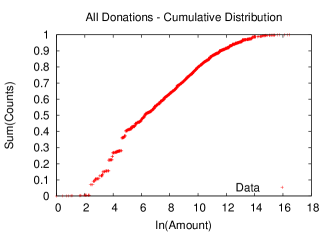
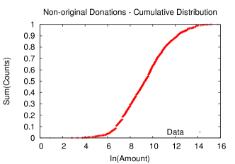
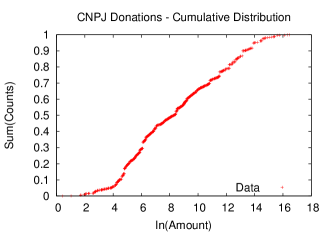
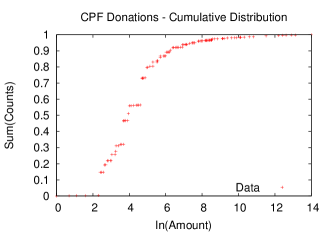
Figure 1: Cumulative distributions for donations declared for the presidential campaigns. Top left: all donations; Top right: non-original donations; Bottom left: CNPJ donations; Bottom right: CPF donations.

Table 1: Statistics for all donations declared for the presidential campaigns.

Donations	Min [R$]	Max [R$]	Average [R$]	STD [R$]	N	Total [R$]
All	1.00	14000000.00	81773.906	435812.697	11400	932222528.31
CNPJ	1.56	14000000.00	252883.227	874317.765	2242	566964194.65
CPF	1.00	1200000.00	2777.926	30722.847	5198	14439660.54
Non-original	2.38	7000000.00	88825.673	297193.854	3949	350772581.57
Unknown	100.00	18826.29	4190.141	5818.040	11	46091.55

Table 2: Statistics for all donations declared by the parties central directories.

Donations	Min [R$]	Max [R$]	Average [R$]	STD [R$]	N	Total [R$]
All	0.02	13000000.00	366917.292	756161.911	2490	913624056.53
CNPJ	30.00	13000000.00	422592.562	802850.503	2129	899699564.27
CPF	0.10	1000000.00	41129.083	133472.945	336	13819371.87
Unknown	0.02	26211.02	4204.816	6714.171	25	105120.39

In figure 2 and table 3 we show the same histograms and statistics, evaluated for the governor regional campaign in one federal unit, the Rio Grande do Sul (RS). Data for the other 26 federal units, shows very similar patterns.

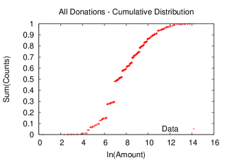
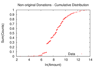
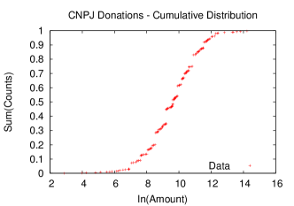
Figure 2: Top: Histogram in logarithmic scale for all donations declared in a regional campaign. Bottom left: only donations from legal entities. Bottom right: only donations from legal persons.

Table 3: Statistics for all donations declared in the RS Governor electoral campaigns.

Type	Min [R$]	Max [R$]	Average [R$]	STD [R$]	N	Total [R$]
All	1.50	1500000.00	17191.173	66018.435	2595	44611094.90
CNPJ	18.00	1500000.00	43165.157	108942.678	545	23525010.55
CPF	1.50	75000.00	1523.075	4530.274	1229	1871859.08
Non-original	14.00	950000.00	23458.969	70986.723	819	19212895.27
Unknown	330.00	1000.00	665.000	473.762	2	1330.00

2.2 Donation Model

In figures 1 and 2 one can see that the cumulative distribution of the donations tend to have a sigmoidal shape when the horizontal axis is in logarithmic scale.

Let’s fit to the cumulative distributions a truncated sigmoidal function. Take the function

$$F(\xi) = \frac{\xi^{\gamma}}{\xi_{0}^{\gamma}+\xi^{\gamma}}=\frac{1}{1+\left(\frac{\xi_{0}}{\xi}\right)^{\gamma}}$$ (3)

$$\xi \in (0;\infty),$$ (4)

where $\gamma$ and $\xi_{0}$ are the parameters to be fitted. In order to shift the minimum possible value of the variable $\xi$, one can make the replacement $\xi\rightarrow\xi-\Delta$ where $\Delta$ is now the new minimum possible value for the variable. In order to truncate the maximum value for the distribution ($F(\xi)$ should be equal to 1 for $\xi_{max}$), one makes the transformation $F(\xi)\rightarrow\frac{F(\xi)}{F(\xi_{max})}$. Since the horizontal axis is in logarithmic scale, the variable of the distribution is related to the amounts ($x$) present in the data by $\xi=\ln(x)$. The actual distribution one needs is the derivative of the cumulative distribution:

$$F(x) = \left\{\begin{array}[]{cc}0.&x<e^{\Delta}\\ \frac{1+\left(\frac{\xi_{0}}{\xi_{max}-\Delta}\right)^{\gamma}}{1+\left(\frac{\xi_{0}}{\xi-\Delta}\right)^{\gamma}}&e^{\Delta}<x<e^{\xi_{max}}\\ 1&x>e^{\xi_{max}}\end{array}\right.$$ (8)

$$f(x) = \frac{\textrm{d}}{\textrm{d}x}F(x)=\frac{\gamma}{x}\left(1+\left(\frac{\xi_{0}}{\xi_{max}-\Delta}\right)^{\gamma}\right)\frac{\left(\frac{\xi_{0}}{\ln(x)-\Delta}\right)^{\gamma}}{\left(1+\left(\frac{\xi_{0}}{\ln(x)-\Delta}\right)^{\gamma}\right)^{2}}\frac{1}{\ln(x)-\Delta}.$$ (9)

Now, given a set of numbers ($x_{i}$, $i=1,2,...,N$) we set $\xi_{max}=\max(x_{i})+1$, $\Delta=log(0.01)$ (the smallest possible donation is one cent) and determine the values of $\xi_{0}$ and $\gamma$ that maximize the likelihood for the set:

$${\cal L} = \prod_{i=1}^{N}f(x_{i})$$ (10)

$$\ln{\cal L} = \displaystyle\sum\limits_{i}f(x_{i})=N\left(\ln\gamma+\ln\left(1+\left(\frac{\xi_{0}}{\xi_{max}-\Delta}\right)^{\gamma}\right)+\gamma\ln\xi_{0}\right)-\displaystyle\sum\limits_{i=1}^{N}\ln x_{i}+$$ (11)

$$- (\gamma+1)\displaystyle\sum\limits_{i=1}^{N}\ln\left(\ln x_{i}-\Delta\right)-2\displaystyle\sum\limits_{i=1}^{N}\ln\left(1+\left(\frac{\xi_{0}}{\ln x_{i}-\Delta}\right)^{\gamma}\right).$$

A steepest ascent algorithm was implemented in order to maximize the likelihood: iteratively, given initial arbitrary values for $\gamma$ and $\xi_{0}$, the gradient of the likelihood in parameter space is evaluated and the values of the parameters are increased (or decreased) by small amounts following this gradient. This iteration is repeated until the norm of the gradient approaches zero (within some numerical precision).

In figure 3, one can see the same distributions from figure 1 with the fitted distributions. The parameters obtained for these fits are in table 4.

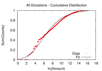
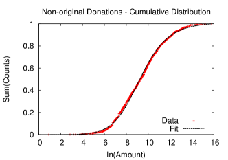
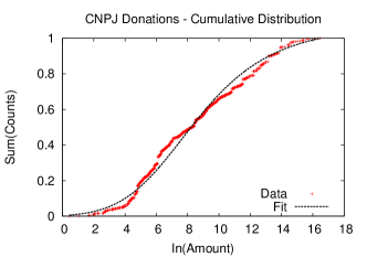
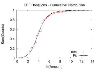
Figure 3: Cumulative distributions for donations declared for the presidential campaigns with fitted distributions. Top left: all donations; Top right: non-original donations; Bottom left: CNPJ donations; Bottom right: CPF donations.

Table 4: Fitted parameters to the distributions in the presidential campaign.

Donations	Max [R$]	N	$\gamma$	$e^{\xi_{0}}$ [R$]
All	14000000.00	11400	5.289261	70747.23
CNPJ	14000000.00	2242	5.334680	539065.67
CPF	1200000.00	5198	10.274493	5463.28
Non-original	7000000.00	3949	10.982049	1068336.77

2.3 Logistic Regression

Before presenting our results on the first digit distribution for the declared donations in the electoral campaigns, we would like to establish the importance this money has in the outcome of the election. For this purpose, we fit a logistic model (logit regression) setting as dependent variable the result of the election for a given candidate (elected or not elected) and as independent variable the fraction of all money declared as donations in the whole campaign for the same office that each candidate received.

The logistic model comes from the assumption that one can determine the probability of success ($p$) in a given process from a set of $k$ predictor factors ($x_{i}$, i=1, 2, …, $k$) with the logistic function[29]:

$$p(x) = \frac{1}{1+e^{-\left(\beta_{0}+\displaystyle\sum\limits_{i=1}^{k}\beta_{i}x_{i}\right)}}$$ (12)

where $p$ is the probability of success, $x_{i}$ are the values of the predictors and $\beta_{i}$ are parameters to be fitted from data. In our case, we fit two parameters, $\beta_{0}$ and $\beta_{1}$ by correlating the probability of a candidate to be elected for office with the total fraction of donations $x_{1}$ received by him during the campaign. In order to obtain the best fit to the model we use Newton-Raphson method in order to obtain the values of the parameters that maximize the likelihood for the observed data given the model.

Regarding the logistic regression, we perform two statistical tests: for each fitted parameter ($\beta_{0}$ and $\beta_{1}$), the Wald test where we compare the ratio between the square of the parameter with its uncertainty against a $\chi^{2}$ distribution with one degree of freedom (this is equivalent to the z-test). Small p-values in this test indicate a significant value for the parameter obtained (that it is in fact different from zero). In another test we evaluate the deviance for the model given the obtained parameters [30] and compare it to a $\chi^{2}$ distribution. This test asserts the overall quality of the fit: high (close to 1) p-values in this test indicate a good fit (a good description of the data by the model).

3 Results and Discussion

For performing the logistic regression analysis, the election results for each one of the 27 Brazilian federal units were obtained. In each federal unit, for each candidate to a given office (we analyze data for the regional and federal congress offices because for these offices many candidates are elected and, therefore, there is enough statistics to perform the analysis) one is able to obtain, from the data, the total amount of money received by him as donations and to know whether he was elected or not.

In table 5 we show the results of the logistic regression fit for the federal congressmen campaign in each one of Brazil’s federal units. It is astonishing how well the model fits the data (p-values associated to the deviance close to 1) and how significant the obtained parameters are (Wald p-values close to 0). This result indicates that money certainly is a good predictor of whether a candidate is elected or not. From these results, the value of $\beta_{1}$ can be used to estimate how more likely (how the odds ratio increase) for a candidate to be elected if he receives an extra amount of money $y$:

$$\textrm{oddR}(y) = \frac{p(x+y)}{p(x)}=e^{\beta_{1}y}$$ (13)

take, for example, the case of federal congress campaign in RS, where $\beta_{1}$=329.49. If a candidate receives a 100000R$ donation, the odds of him being elected increase $e^{\frac{100000*329.49}{55096519.3}}=1.82$. In other words, the odds of being elected raise by 82% every 100000R$ a candidate receives as donation. And receiving nothing, the chances of being elected are $p(0)=0.0133$ (around 1.3%).

Table 5: Results for the logistic regression fits for the federal congress elections. For each federal unit (UF), the first line show the value for the fitted intercept ($\beta_{0}$) with its uncertainty and the correspondent Wald p-value and the second line shows the values for the parameter associated with the money variable ($\beta_{1}$) with its correspondent uncertainty and p-value. The column $N$ shows the number of candidates and the column $n$ the number disputed chairs (elected candidates). The last p-value column is the result for the test performed with the deviance parameter that reflects the overall quality of the fit. In the last column we present the total amount of money donated for the campaigns in each UF.

UF	$\beta\pm\sigma$	p-value (Wald)	$N$	$n$	Deviance	p-value	Total Money [R$]
RS	-4.301740 $\pm$ 0.485408	0.000000	308	31	74.527927	1.000000	55096519.30
	329.493809 $\pm$ 52.566813	0.000000
AC	-3.449199 $\pm$ 0.757419	0.000005	62	8	32.333029	0.998680	8413305.29
	55.166227 $\pm$ 16.037827	0.000582
AL	-4.695802 $\pm$ 0.990996	0.000002	100	9	20.127256	1.000000	17400034.17
	92.585381 $\pm$ 23.365122	0.000074
AM	-4.707182 $\pm$ 1.167616	0.000055	79	8	17.908722	1.000000	22986481.15
	91.221557 $\pm$ 26.302040	0.000524
AP	-2.867302 $\pm$ 0.437003	0.000000	104	8	49.453531	0.999998	8668201.78
	22.829906 $\pm$ 10.653730	0.032121
BA	-3.896939 $\pm$ 0.407161	0.000000	312	39	90.934608	1.000000	71157732.26
	418.617858 $\pm$ 64.287666	0.000000
CE	-3.503933 $\pm$ 0.433627	0.000000	195	22	74.903382	1.000000	34860757.57
	137.942303 $\pm$ 23.606311	0.000000
DF	-4.313380 $\pm$ 0.756930	0.000000	128	8	36.354865	1.000000	19218865.40
	78.962065 $\pm$ 18.805065	0.000027
ES	-4.124638 $\pm$ 0.619728	0.000000	157	10	41.305258	1.000000	18836757.57
	87.468974 $\pm$ 19.952579	0.000012
GO	-3.070569 $\pm$ 0.534978	0.000000	95	17	51.188912	0.999870	63643888.31
	93.675674 $\pm$ 20.562509	0.000005
MA	-3.128799 $\pm$ 0.334342	0.000000	235	18	102.435737	1.000000	21227657.48
	79.044032 $\pm$ 19.063608	0.000034
MG	-4.252349 $\pm$ 0.337550	0.000000	620	53	141.959135	1.000000	158630223.27
	503.226068 $\pm$ 56.348581	0.000000
MS	-5.973087 $\pm$ 1.580883	0.000158	116	8	14.792692	1.000000	29169885.35
	128.623347 $\pm$ 35.197929	0.000258
MT	-4.494480 $\pm$ 0.947234	0.000002	96	8	21.760442	1.000000	25722371.33
	83.391765 $\pm$ 23.946738	0.000497
PA	-3.764366 $\pm$ 0.507372	0.000000	174	17	64.372699	1.000000	19237189.65
	129.209794 $\pm$ 24.536572	0.000000
PB	-4.795535 $\pm$ 1.083687	0.000010	96	12	17.658204	1.000000	13639599.77
	157.281575 $\pm$ 44.818445	0.000449
PE	-2.897830 $\pm$ 0.380326	0.000000	155	25	85.841997	0.999998	50791711.79
	126.721817 $\pm$ 23.957652	0.000000
PI	-3.362935 $\pm$ 0.626560	0.000000	88	10	38.131270	0.999998	24434149.38
	80.046119 $\pm$ 23.186551	0.000556
PR	-3.522870 $\pm$ 0.348306	0.000000	295	30	99.829366	1.000000	69943697.86
	198.013071 $\pm$ 31.148521	0.000000
RJ	-4.309115 $\pm$ 0.278953	0.000000	953	46	182.068165	1.000000	109193461.16
	497.533828 $\pm$ 56.288402	0.000000
RN	-5.692015 $\pm$ 1.756848	0.001196	83	8	13.736874	1.000000	14278235.86
	110.857108 $\pm$ 35.288882	0.001681
RO	-3.420208 $\pm$ 0.646803	0.000000	81	8	35.803050	0.999993	17001787.46
	56.756842 $\pm$ 18.389173	0.002026
RR	-4.050292 $\pm$ 0.846561	0.000002	80	8	25.829202	1.000000	8356682.91
	96.267954 $\pm$ 29.868455	0.001268
SC	-3.715785 $\pm$ 0.579054	0.000000	128	16	49.832673	1.000000	31737303.92
	115.394467 $\pm$ 23.029840	0.000001
SE	-2.981286 $\pm$ 0.564645	0.000000	73	8	36.331160	0.999795	7622064.24
	37.830953 $\pm$ 13.895874	0.006480
SP	-4.113540 $\pm$ 0.215463	0.000000	1318	70	301.879103	1.000000	234478433.27
	551.467211 $\pm$ 47.421220	0.000000
TO	-3.353321 $\pm$ 0.853338	0.000085	47	8	25.137784	0.992752	14895843.70
	53.979352 $\pm$ 17.658840	0.002237

In Table 6 we show the results of the logistic regression for the regional congress office seats.

Table 6: Results for the logistic regression fits for the regional congress elections. For each federal unit (UF), the first line show the value for the fitted intercept ($\beta_{0}$) with its uncertainty and the correspondent Wald p-value and the second line shows the values for the parameter associated with the money variable ($\beta_{1}$) with its correspondent uncertainty and p-value. The column $N$ shows the number of candidates and the column $n$ the number of disputed chairs (elected candidates). The last p-value column is the result for the test performed with the deviance parameter that reflects the overall quality of the fit. In the last column we present the total amount of money donated for the campaigns in each UF.

UF	$\beta\pm\sigma$	p-value (Wald)	$N$	$n$	Deviance	p-value	Total Money [R$]
RS	-3.895895 $\pm$ 0.268780	0.000000	670	55	229.721642	1.000000	53897470.35
	520.063531 $\pm$ 57.562793	0.000000
AC	-4.268271 $\pm$ 0.368601	0.000000	497	24	122.215355	1.000000	10741882.23
	281.612445 $\pm$ 42.665487	0.000000
AL	-3.855591 $\pm$ 0.433952	0.000000	262	27	93.457895	1.000000	19512010.69
	211.488057 $\pm$ 31.624984	0.000000
AM	-5.421684 $\pm$ 0.560394	0.000000	570	24	76.805367	1.000000	24576432.18
	416.471023 $\pm$ 60.800589	0.000000
AP	-3.838433 $\pm$ 0.373426	0.000000	338	24	112.245178	1.000000	5621758.62
	206.887652 $\pm$ 34.012981	0.000000
BA	-3.591355 $\pm$ 0.260449	0.000000	578	63	235.229572	1.000000	47098049.37
	488.121206 $\pm$ 54.578145	0.000000
CE	-3.866844 $\pm$ 0.296504	0.000000	558	46	177.125300	1.000000	32583088.46
	368.870924 $\pm$ 42.414498	0.000000
DF	-4.473329 $\pm$ 0.292542	0.000000	979	24	158.940820	1.000000	35648405.99
	261.270656 $\pm$ 40.316546	0.000000
ES	-4.086863 $\pm$ 0.350796	0.000000	472	30	138.579334	1.000000	23230725.98
	285.100562 $\pm$ 37.708774	0.000000
GO	-3.736298 $\pm$ 0.245030	0.000000	717	41	211.477478	1.000000	79100331.98
	270.582549 $\pm$ 32.741606	0.000000
MA	-4.304746 $\pm$ 0.386074	0.000000	490	42	119.106959	1.000000	25769715.01
	470.819026 $\pm$ 60.737138	0.000000
MG	-3.812026 $\pm$ 0.209294	0.000000	1055	77	325.294508	1.000000	141181882.89
	571.563491 $\pm$ 49.725496	0.000000
MS	-5.025201 $\pm$ 0.569786	0.000000	395	24	69.193927	1.000000	45931385.85
	338.506140 $\pm$ 51.048838	0.000000
MT	-3.863263 $\pm$ 0.404347	0.000000	292	24	100.184791	1.000000	51160968.29
	199.266811 $\pm$ 30.810483	0.000000
PA	-3.599082 $\pm$ 0.243462	0.000000	650	41	223.961945	1.000000	31697472.64
	276.652126 $\pm$ 36.713893	0.000000
PB	-4.058142 $\pm$ 0.418954	0.000000	333	36	110.491532	1.000000	17238137.47
	315.883453 $\pm$ 40.915450	0.000000
PE	-3.656680 $\pm$ 0.288765	0.000000	489	49	175.615591	1.000000	40611046.64
	342.514907 $\pm$ 39.141519	0.000000
PI	-5.604635 $\pm$ 0.884008	0.000000	226	30	57.843668	1.000000	20247713.90
	412.376534 $\pm$ 69.711243	0.000000
PR	-4.621801 $\pm$ 0.348345	0.000000	738	54	166.557103	1.000000	61112695.05
	692.209375 $\pm$ 71.533492	0.000000
RJ	-4.316389 $\pm$ 0.199879	0.000000	1846	70	342.421533	1.000000	129527220.71
	630.840620 $\pm$ 54.192459	0.000000
RN	-4.152926 $\pm$ 0.509765	0.000000	244	24	69.343989	1.000000	18313268.55
	198.547307 $\pm$ 30.987689	0.000000
RO	-3.658539 $\pm$ 0.325359	0.000000	382	24	130.082195	1.000000	25257051.30
	176.974288 $\pm$ 30.220810	0.000000
RR	-4.162472 $\pm$ 0.394217	0.000000	393	24	100.233152	1.000000	13405608.74
	227.670731 $\pm$ 32.618995	0.000000
SC	-3.662375 $\pm$ 0.315007	0.000000	409	40	159.849890	1.000000	51935831.01
	323.898860 $\pm$ 43.323434	0.000000
SE	-3.379372 $\pm$ 0.456329	0.000000	162	24	83.869900	1.000000	8427039.38
	161.551846 $\pm$ 28.397770	0.000000
SP	-4.193506 $\pm$ 0.185004	0.000000	1878	94	432.635429	1.000000	229364470.60
	836.922136 $\pm$ 60.696497	0.000000
TO	-4.478863 $\pm$ 0.587435	0.000000	238	24	74.147005	1.000000	19956645.63
	290.774731 $\pm$ 50.526507	0.000000

The results clearly indicate that money is an excellent predictor of whether a given candidate will be elected for office or not. Note, that the model deals with probabilities, so we are not saying that the ones who receive more money are surely elected; what the analysis shows is that the more money a candidate receives, the more probable it is for him to be elected. This might (sadly) sound like an obvious statement, but this actually obliterates the principle of democracy: our representatives are not elected because they represent our interests, they are elected because they gather huge amounts of money in order to hire marketing professionals and flood media time with spurious publicity. In other words, candidates know that, to get elected, they do not need to have previously done a good job, to have developed good projects or even to be honest, the most important thing they need is to get money, lots of it.

It could be possible try and argue that the candidates that receive the most money are those that better represent the population, since it is the population that makes the donations. Actually, most of the money comes from legal entities (CNPJ) or from the parties (non-original) which recieved most of their money from companies. Moreover, it is common knowledge that most parties and candidates receive unofficial donations (in Portuguese referred to by the term “caixa dois”, second cashier) that must pass through some kind of money laundry before being used. It is quite easy to compare the huge amounts donated by companies with plain bribes: the candidates, once elected, legislate beneficial laws to help those economic sectors that helped them to be elected in the first place; from the companies point of view, the donations are investments [31].

The next analysis is based on the idea that the set of numbers in an honest financial declaration should follow the Benford’s law for the first significant digit distribution. Some arguments for that have already been presented: the declarator should have no real control over the amounts (random donations) and the amounts expand many orders of magnitude and come from multiple different distributions. Therefore, deviations of Benford’s law would be evidence of fraud, indications that the declaration has been “cooked” (money laundry).

In table 7 we show the first significant digit distribution for all donations received by each political party specifically for the 2014 presidential campaign. For each party, we present the results for all donations together and then for the amounts classified according to the donor (CNPJ, CPF, non-original). We also present results for artificial data generated from the distributions fitted to each data set; those are indicated by the tag _Rand and in the last line, for each party, indicated by the tag _Model, is the result for the different sets of artificial data for each category combined. In this analysis, we have considered only sets of data with more than 20 elements (some parties or some specific categories in a given party that are not shown in the table, had $N<20$ and were omitted). In table 8 we present a similar table for all the donations declared by each political party central directory. These are the donations that end up distributed as non-original to various campaigns.

The $\chi^{2}$ values in the table are calculated via:

$$\chi^{2} = \sum_{i=1}^{9}N\frac{(O_{i}-E_{i})^{2}}{E_{i}}$$ (14)

where $O_{i}$ is the observed frequency of each digit, $E_{i}$ is the expected frequency according to Benford’s Law and $N$ is the total number of elements in the analyzed set. The p-values are the probabilities that a fluctuation equal or bigger than the observed $\chi^{2}$ may be obtained in a set of numbers of the same size that do agree with the Benford empirical distribution.

Table 7: First significant digit distribution for all donations received for the presidential campaign by the different parties. The columns 1-9 indicate the proportion each one of the nine digits is observed, N the total number of donations, $\chi^{2}$ is the statistic for the fluctuation, p-val its correspondent p-value, Min and Max are respectively the minimum and maximum amounts donated and sum is the sum of all donations, $\gamma$ and $\xi_{0}$ are the model parameters.

Partido	1	2	3	4	5	6	7	8	9	N	$\chi^{2}$	p-val	Min	Max	Sum	$\gamma$	$\xi_{0}$
Benford	0.301	0.176	0.125	0.097	0.079	0.067	0.058	0.051	0.046
PSDB - All	0.304	0.183	0.115	0.091	0.088	0.060	0.049	0.068	0.043	3545	36.968	0.000	17.00	14000000.00	428137499.87	10.6744	13.9580
PSDB - All Rand	0.292	0.181	0.129	0.092	0.084	0.065	0.054	0.049	0.054	3545	10.023	0.263	10.58	13553439.45	647168618.07	10.6744	13.9580
PSDB - CNPJ	0.263	0.222	0.080	0.086	0.198	0.047	0.027	0.038	0.038	338	81.172	0.000	20.00	14000000.00	176814668.46	9.9850	16.4027
PSDB - CNPJ Rand	0.243	0.180	0.151	0.080	0.077	0.053	0.071	0.080	0.065	338	16.872	0.031	127.87	13656868.89	290580085.73	9.9850	16.4027
PSDB - CPF	0.268	0.390	0.098	0.049	0.122	0.016	0.049	0.000	0.008	123	53.990	0.000	450.00	1200000.00	7933331.08	11.4890	13.3403
PSDB - CPF Rand	0.285	0.228	0.138	0.073	0.057	0.049	0.041	0.049	0.081	123	8.280	0.407	105.78	428568.20	4612216.49	11.4890	13.3403
PSDB - Non-original	0.310	0.169	0.120	0.093	0.074	0.063	0.051	0.074	0.045	3078	39.221	0.000	17.00	7000000.00	243369609.95	11.1858	13.7907
PSDB - Non-original Rand	0.305	0.187	0.126	0.090	0.083	0.069	0.048	0.048	0.045	3078	9.838	0.277	3.77	6998795.84	322481463.76	11.1858	13.7907
PSDB - Model	0.298	0.188	0.129	0.089	0.081	0.067	0.050	0.051	0.048	3545	9.759	0.282	3.77	13656868.89	622410419.10	-	-
PV - All	0.267	0.206	0.170	0.079	0.109	0.042	0.067	0.030	0.030	165	10.517	0.231	1.56	1000000.00	7922280.69	5.9339	12.0622
PV - All Rand	0.352	0.152	0.145	0.055	0.103	0.048	0.061	0.042	0.042	165	7.905	0.443	0.48	979516.62	5255748.70	5.9339	12.0622
PV - CNPJ	0.242	0.226	0.169	0.089	0.056	0.056	0.081	0.040	0.040	124	7.698	0.464	1.56	1000000.00	7893364.47	5.5143	13.2271
PV - CNPJ Rand	0.339	0.153	0.113	0.105	0.081	0.073	0.065	0.024	0.048	124	3.111	0.927	0.95	935712.73	10042984.38	5.5143	13.2271
PV - CPF	0.341	0.146	0.171	0.049	0.268	0.000	0.024	0.000	0.000	41	28.131	0.000	10.00	7000.00	28916.22	9.9028	10.0454
PV - CPF Rand	0.268	0.317	0.049	0.073	0.049	0.122	0.049	0.073	0.000	41	11.572	0.171	6.36	5294.41	28733.08	9.9028	10.0454
PV - Model	0.321	0.194	0.097	0.097	0.073	0.085	0.061	0.036	0.036	165	3.475	0.901	0.95	935712.73	10071717.47	-	-
PSTU - All	0.496	0.141	0.133	0.067	0.081	0.030	0.015	0.022	0.015	135	31.598	0.000	20.00	20000.00	171676.75	9.7162	10.1468
PSTU - All Rand	0.281	0.178	0.148	0.081	0.104	0.067	0.052	0.037	0.052	135	2.836	0.944	3.61	15837.56	109612.51	9.7162	10.1468
PSTU - CPF	0.546	0.102	0.139	0.074	0.083	0.028	0.009	0.000	0.019	108	39.909	0.000	20.00	20000.00	104045.00	11.1369	9.7449
PSTU - CPF Rand	0.306	0.222	0.176	0.074	0.046	0.056	0.019	0.056	0.046	108	8.769	0.362	2.16	5493.99	46241.56	11.1369	9.7449
PSTU - Model	0.356	0.200	0.148	0.067	0.044	0.044	0.030	0.059	0.052	135	8.862	0.354	2.16	19258.32	320209.16	-	-
PT - All	0.411	0.182	0.059	0.071	0.170	0.022	0.034	0.028	0.022	3024	751.337	0.000	1.00	10000000.00	351270140.26	6.1549	10.4056
PT - All Rand	0.303	0.182	0.126	0.091	0.080	0.070	0.063	0.045	0.040	3024	8.129	0.421	0.11	9993290.98	241002479.22	6.1549	10.4056
PT - CNPJ	0.365	0.133	0.090	0.129	0.099	0.040	0.061	0.053	0.031	1478	96.414	0.000	2.80	10000000.00	307721104.56	5.8880	11.8043
PT - CNPJ Rand	0.317	0.172	0.136	0.085	0.077	0.062	0.066	0.046	0.039	1478	9.835	0.277	0.20	9919764.38	245410372.53	5.8880	11.8043
PT - CPF	0.485	0.235	0.007	0.004	0.264	0.002	0.002	0.001	0.002	1320	1290.454	0.000	1.00	500000.00	869017.00	11.3187	8.8406
PT - CPF Rand	0.278	0.181	0.137	0.091	0.076	0.069	0.067	0.053	0.048	1320	6.855	0.552	1.01	62840.98	466397.20	11.3187	8.8406
PT - Non-original	0.283	0.195	0.159	0.088	0.084	0.031	0.044	0.027	0.088	226	19.852	0.011	16.20	3800000.00	42680018.70	10.3475	14.7289
PT - Non-original Rand	0.367	0.133	0.128	0.088	0.088	0.040	0.071	0.035	0.049	226	10.399	0.238	15.32	3722448.46	35609479.64	10.3475	14.7289
PT - Model	0.304	0.173	0.136	0.088	0.077	0.063	0.067	0.048	0.044	3024	11.365	0.182	0.20	9919764.38	281486249.37	-	-
PSB - All	0.472	0.132	0.040	0.244	0.077	0.011	0.014	0.005	0.006	3876	2104.931	0.000	1.00	5000000.00	123023025.46	6.6782	9.0822
PSB - All Rand	0.303	0.174	0.117	0.102	0.079	0.068	0.061	0.049	0.047	3876	4.537	0.806	0.13	4708204.53	55901564.13	6.6782	9.0822
PSB - CNPJ	0.353	0.199	0.096	0.038	0.212	0.032	0.045	0.000	0.026	156	55.538	0.000	13.33	5000000.00	54326607.36	5.8168	17.5564
PSB - CNPJ Rand	0.301	0.103	0.154	0.115	0.071	0.071	0.071	0.051	0.064	156	8.129	0.421	6.25	4697620.88	80401952.53	5.8168	17.5564
PSB - CPF	0.508	0.118	0.018	0.282	0.065	0.004	0.003	0.002	0.001	3142	2560.399	0.000	1.00	500000.00	5387549.24	11.1146	8.4009
PSB - CPF Rand	0.281	0.194	0.128	0.101	0.079	0.067	0.056	0.050	0.043	3142	11.228	0.189	0.15	304842.86	1492020.92	11.1146	8.4009
PSB - Non-original	0.307	0.186	0.141	0.085	0.106	0.047	0.068	0.026	0.033	574	21.131	0.007	2.38	3000000.00	63301493.98	11.2112	14.3195
PSB - Non-original Rand	0.287	0.179	0.157	0.111	0.068	0.075	0.045	0.040	0.037	574	11.799	0.160	26.64	2661538.45	67001138.08	11.2112	14.3195
PSB - Model	0.282	0.188	0.133	0.103	0.077	0.069	0.055	0.049	0.043	3876	13.331	0.101	0.15	4697620.88	148977209.29	-	-
PDT - All	0.291	0.236	0.164	0.091	0.073	0.055	0.036	0.018	0.036	55	3.707	0.883	4000.00	2000000.00	18938826.29	15.0178	16.6327
PDT - All Rand	0.236	0.200	0.127	0.036	0.109	0.109	0.055	0.055	0.073	55	6.004	0.647	1210.40	1913866.96	13948573.89	15.0178	16.6327
PDT - CNPJ	0.278	0.241	0.167	0.093	0.074	0.056	0.037	0.019	0.037	54	3.887	0.867	4000.00	2000000.00	18920000.00	15.1149	16.6790
PDT - CNPJ Rand	0.241	0.130	0.093	0.130	0.074	0.093	0.093	0.074	0.074	54	5.527	0.700	835.23	1822964.94	18306741.04	15.1149	16.6790
PDT - Model	0.255	0.127	0.091	0.127	0.073	0.091	0.091	0.073	0.073	55	5.075	0.750	835.23	1822964.94	19328360.54	-	-
PRTB - All	0.328	0.138	0.155	0.069	0.069	0.086	0.000	0.000	0.155	58	23.410	0.003	43.30	100000.00	440985.26	11.1681	11.5622
PRTB - All Rand	0.190	0.138	0.172	0.103	0.121	0.017	0.155	0.034	0.069	58	17.787	0.023	16.16	54157.04	246427.41	11.1681	11.5622
PRTB - Non-original	0.368	0.105	0.132	0.079	0.079	0.105	0.000	0.000	0.132	38	12.893	0.116	43.30	100000.00	195090.32	12.5753	11.3702
PRTB - Non-original Rand	0.289	0.368	0.079	0.053	0.105	0.026	0.000	0.079	0.000	38	15.191	0.056	29.20	87262.96	367477.89	12.5753	11.3702
PRTB - Model	0.259	0.310	0.052	0.052	0.086	0.052	0.086	0.069	0.034	58	11.548	0.173	29.20	90014.86	1238572.93	-	-
PCB - All	0.273	0.152	0.121	0.152	0.000	0.152	0.061	0.061	0.030	33	7.592	0.474	70.00	16000.00	60554.69	13.5250	11.1803
PCB - All Rand	0.303	0.212	0.121	0.061	0.030	0.182	0.030	0.000	0.061	33	10.480	0.233	54.45	3125.84	35234.71	13.5250	11.1803
PSOL - All	0.437	0.265	0.028	0.006	0.251	0.002	0.004	0.004	0.002	471	393.503	0.000	1.00	94953.74	401555.67	9.8255	8.4428
PSOL - All Rand	0.291	0.195	0.123	0.072	0.079	0.064	0.062	0.053	0.062	471	6.923	0.545	1.50	14644.12	129531.55	9.8255	8.4428
PSOL - CNPJ	0.167	0.417	0.000	0.042	0.208	0.000	0.083	0.042	0.042	24	20.061	0.010	18.40	94953.74	246919.27	9.8356	13.0237
PSOL - CNPJ Rand	0.542	0.167	0.042	0.083	0.042	0.000	0.083	0.000	0.042	24	9.542	0.299	56.21	43474.71	261107.25	9.8356	13.0237
PSOL - CPF	0.451	0.260	0.027	0.005	0.255	0.002	0.000	0.000	0.000	443	393.235	0.000	1.00	12000.00	103538.00	11.1878	8.3139
PSOL - CPF Rand	0.300	0.187	0.120	0.088	0.081	0.050	0.070	0.052	0.052	443	4.251	0.834	0.25	8307.16	71625.52	11.1878	8.3139
PSOL - Model	0.316	0.185	0.115	0.087	0.079	0.047	0.070	0.049	0.053	471	6.106	0.635	0.25	43474.71	363857.42	-	-

Table 8: First significant digit distribution for all donations received for the presidential campaign by the different parties. The columns 1-9 indicate the proportion each one of the nine digits is observed, N the total number of donations, $\chi^{2}$ is the statistic for the fluctuation, p-val its correspondent p-value, Min and Max are respectively the minimum and maximum amounts donated and sum is the sum of all donations.

Partido	1	2	3	4	5	6	7	8	9	N	$\chi^{2}$	p-val	Min	Max	Sum
Benford	0.301	0.176	0.125	0.097	0.079	0.067	0.058	0.051	0.046
PT do B - All	0.417	0.000	0.083	0.000	0.333	0.000	0.167	0.000	0.000	12	18.175	0.020	1200.00	105000.00	408402.23
PT do B - CNPJ	0.417	0.000	0.083	0.000	0.333	0.000	0.167	0.000	0.000	12	18.175	0.020	1200.00	105000.00	408402.23
PEN - All	0.667	0.000	0.000	0.000	0.333	0.000	0.000	0.000	0.000	3	5.639	0.688	1500.00	500000.00	503000.00
PEN - CNPJ	0.000	0.000	0.000	0.000	1.000	0.000	0.000	0.000	0.000	1	11.629	0.169	500000.00	500000.00	500000.00
PEN - CPF	1.000	0.000	0.000	0.000	0.000	0.000	0.000	0.000	0.000	2	4.644	0.795	1500.00	1500.00	3000.00
DEM - All	0.364	0.193	0.107	0.079	0.179	0.021	0.021	0.021	0.014	140	33.400	0.000	600.00	3300000.00	51921770.00
DEM - CNPJ	0.350	0.197	0.109	0.080	0.182	0.022	0.022	0.022	0.015	137	32.995	0.000	600.00	3300000.00	51621770.00
DEM - CPF	1.000	0.000	0.000	0.000	0.000	0.000	0.000	0.000	0.000	3	6.966	0.540	100000.00	100000.00	300000.00
PMDB - All	0.302	0.181	0.129	0.055	0.189	0.031	0.058	0.024	0.031	381	79.460	0.000	1513.58	7000000.00	186799588.38
PMDB - CNPJ	0.318	0.188	0.128	0.045	0.176	0.031	0.060	0.026	0.028	352	65.570	0.000	3000.95	7000000.00	182368186.61
PMDB - CPF	0.103	0.103	0.138	0.172	0.345	0.034	0.034	0.000	0.069	29	34.778	0.000	1513.58	1000000.00	4431401.77
PR - All	0.339	0.271	0.059	0.085	0.203	0.025	0.008	0.000	0.008	118	51.511	0.000	542.39	5000000.00	63275909.49
PR - CNPJ	0.339	0.284	0.064	0.083	0.193	0.018	0.009	0.000	0.009	109	46.059	0.000	2500.00	5000000.00	62324300.02
PR - CPF	0.333	0.167	0.000	0.000	0.333	0.167	0.000	0.000	0.000	6	8.070	0.427	5000.00	650000.00	930000.00
PTN - All	0.292	0.167	0.042	0.125	0.083	0.000	0.250	0.042	0.000	24	19.556	0.012	21.38	800000.00	5659820.94
PTN - CNPJ	0.250	0.062	0.062	0.188	0.062	0.000	0.375	0.000	0.000	16	33.569	0.000	50000.00	731000.00	4854350.00
PTN - CPF	0.667	0.000	0.000	0.000	0.000	0.000	0.000	0.333	0.000	3	7.946	0.439	100.00	800000.00	800200.00
PP - All	0.266	0.210	0.153	0.048	0.218	0.024	0.040	0.024	0.016	124	43.363	0.000	10000.00	13000000.00	72497495.13
PP - CNPJ	0.254	0.213	0.156	0.049	0.221	0.025	0.041	0.025	0.016	122	44.621	0.000	10000.00	13000000.00	72297495.13
PP - CPF	1.000	0.000	0.000	0.000	0.000	0.000	0.000	0.000	0.000	2	4.644	0.795	100000.00	100000.00	200000.00
PV - All	0.354	0.228	0.114	0.114	0.076	0.038	0.025	0.025	0.025	79	6.471	0.595	10.00	1000000.00	7909375.23
PV - CNPJ	0.346	0.231	0.115	0.115	0.077	0.038	0.026	0.026	0.026	78	6.224	0.622	228.62	1000000.00	7909365.23
PV - CPF	1.000	0.000	0.000	0.000	0.000	0.000	0.000	0.000	0.000	1	2.322	0.970	10.00	10.00	10.00
PT - All	0.379	0.177	0.127	0.042	0.169	0.023	0.044	0.023	0.016	385	84.742	0.000	10.00	10000000.00	191128848.27
PT - CNPJ	0.378	0.182	0.133	0.044	0.155	0.022	0.047	0.025	0.014	362	68.508	0.000	326.26	10000000.00	188973838.27
PT - CPF	0.391	0.087	0.043	0.000	0.391	0.043	0.000	0.000	0.043	23	36.111	0.000	10.00	500000.00	2155010.00
PRB - All	0.500	0.158	0.158	0.040	0.119	0.010	0.010	0.005	0.000	202	75.135	0.000	0.02	1000000.00	10518326.73
PRB - CNPJ	0.319	0.250	0.111	0.083	0.181	0.014	0.028	0.014	0.000	72	21.317	0.006	4000.00	1000000.00	10506015.10
PRB - CPF	0.619	0.095	0.183	0.008	0.087	0.008	0.000	0.000	0.000	126	86.824	0.000	10.00	500.00	4865.00
PTC - All	0.000	0.000	0.000	0.500	0.500	0.000	0.000	0.000	0.000	2	9.474	0.304	50000.00	400000.00	450000.00
PTC - CNPJ	0.000	0.000	0.000	0.500	0.500	0.000	0.000	0.000	0.000	2	9.474	0.304	50000.00	400000.00	450000.00
PTB - All	0.267	0.333	0.167	0.033	0.167	0.000	0.033	0.000	0.000	30	14.129	0.078	10000.00	1300000.00	8810000.00
PTB - CNPJ	0.267	0.333	0.167	0.033	0.167	0.000	0.033	0.000	0.000	30	14.129	0.078	10000.00	1300000.00	8810000.00
PPL - All	0.143	0.143	0.429	0.000	0.143	0.000	0.000	0.000	0.143	7	9.503	0.302	30.12	333403.93	439890.53
PPL - CNPJ	0.250	0.000	0.500	0.000	0.000	0.000	0.000	0.000	0.250	4	10.298	0.245	90.00	333403.93	437360.41
PPL - CPF	0.000	0.500	0.000	0.000	0.500	0.000	0.000	0.000	0.000	2	7.154	0.520	500.00	2000.00	2500.00
PPS - All	0.320	0.200	0.120	0.040	0.240	0.000	0.040	0.000	0.040	25	12.227	0.141	500.15	500000.00	2598945.87
PPS - CNPJ	0.263	0.158	0.158	0.053	0.263	0.000	0.053	0.000	0.053	19	11.071	0.198	30000.00	500000.00	2545000.00
PPS - CPF	0.500	0.500	0.000	0.000	0.000	0.000	0.000	0.000	0.000	4	5.001	0.757	1500.00	20000.00	51500.00
PRP - All	0.000	0.500	0.500	0.000	0.000	0.000	0.000	0.000	0.000	2	4.841	0.774	2500.00	300000.00	302500.00
PRP - CNPJ	0.000	0.000	1.000	0.000	0.000	0.000	0.000	0.000	0.000	1	7.004	0.536	300000.00	300000.00	300000.00
PRP - CPF	0.000	1.000	0.000	0.000	0.000	0.000	0.000	0.000	0.000	1	4.679	0.791	2500.00	2500.00	2500.00
PMN - All	0.133	0.233	0.267	0.167	0.067	0.000	0.033	0.033	0.067	30	12.546	0.128	30.00	1300000.00	2485542.30
PMN - CNPJ	0.148	0.259	0.296	0.074	0.074	0.000	0.037	0.037	0.074	27	12.247	0.141	30.00	1300000.00	2472242.30
PMN - CPF	0.000	0.000	0.000	1.000	0.000	0.000	0.000	0.000	0.000	3	27.957	0.000	4100.00	4700.00	13300.00
PSDC - All	0.214	0.286	0.071	0.000	0.214	0.143	0.000	0.071	0.000	14	8.980	0.344	185.96	100000.00	165885.96
PSDC - CNPJ	0.231	0.308	0.077	0.000	0.154	0.154	0.000	0.077	0.000	13	6.891	0.548	185.96	100000.00	165385.96
PSDC - CPF	0.000	0.000	0.000	0.000	1.000	0.000	0.000	0.000	0.000	1	11.629	0.169	500.00	500.00	500.00
PSDB - All	0.322	0.221	0.109	0.057	0.169	0.044	0.044	0.025	0.008	366	69.617	0.000	0.10	9000000.00	156718898.33
PSDB - CNPJ	0.307	0.226	0.120	0.060	0.166	0.039	0.048	0.024	0.009	332	59.653	0.000	935.06	9000000.00	152093150.51
PSDB - CPF	0.536	0.143	0.000	0.036	0.214	0.036	0.000	0.036	0.000	28	19.777	0.011	0.10	1000000.00	4561050.10
PDT - All	0.111	0.222	0.667	0.000	0.000	0.000	0.000	0.000	0.000	9	25.909	0.001	30000.00	350000.00	1050000.00
PDT - CNPJ	0.111	0.222	0.667	0.000	0.000	0.000	0.000	0.000	0.000	9	25.909	0.001	30000.00	350000.00	1050000.00
PRTB - All	0.211	0.053	0.158	0.105	0.263	0.158	0.053	0.000	0.000	19	14.661	0.066	50.00	31200.00	156631.94
PRTB - CNPJ	0.222	0.056	0.167	0.111	0.278	0.167	0.000	0.000	0.000	18	16.573	0.035	50.00	31200.00	155907.94
PRTB - CPF	0.000	0.000	0.000	0.000	0.000	0.000	1.000	0.000	0.000	1	16.244	0.039	724.00	724.00	724.00
PSL - All	0.340	0.191	0.149	0.043	0.170	0.064	0.000	0.021	0.021	47	11.042	0.199	1500.00	400000.00	1777990.00
PSL - CNPJ	0.340	0.191	0.149	0.043	0.170	0.064	0.000	0.021	0.021	47	11.042	0.199	1500.00	400000.00	1777990.00
PSTU - All	0.400	0.200	0.000	0.000	0.000	0.400	0.000	0.000	0.000	5	10.743	0.217	1986.00	18000.00	35031.08
PSTU - CNPJ	0.333	0.000	0.000	0.000	0.000	0.667	0.000	0.000	0.000	3	18.024	0.021	6000.00	18000.00	30995.08
PSTU - CPF	0.500	0.500	0.000	0.000	0.000	0.000	0.000	0.000	0.000	2	2.500	0.962	1986.00	2050.00	4036.00
PSB - All	0.190	0.171	0.124	0.076	0.324	0.038	0.029	0.019	0.029	105	89.765	0.000	6270.32	3000000.00	35986511.21
PSB - CNPJ	0.192	0.173	0.125	0.077	0.327	0.038	0.029	0.019	0.019	104	91.587	0.000	6270.32	3000000.00	35896511.21
PSB - CPF	0.000	0.000	0.000	0.000	0.000	0.000	0.000	0.000	1.000	1	20.854	0.008	90000.00	90000.00	90000.00
PSC - All	0.304	0.152	0.109	0.043	0.304	0.022	0.022	0.000	0.043	46	35.862	0.000	150.00	1050000.00	5906900.99
PSC - CNPJ	0.268	0.146	0.122	0.024	0.341	0.024	0.024	0.000	0.049	41	42.213	0.000	10000.00	1050000.00	5899650.99
PSC - CPF	0.600	0.200	0.000	0.200	0.000	0.000	0.000	0.000	0.000	5	4.179	0.841	150.00	4900.00	7250.00
PCO - All	0.500	0.000	0.000	0.000	0.000	0.000	0.000	0.500	0.000	2	9.436	0.307	83.33	100.00	183.33
PCO - CNPJ	0.500	0.000	0.000	0.000	0.000	0.000	0.000	0.500	0.000	2	9.436	0.307	83.33	100.00	183.33
PROS - All	0.000	0.000	0.500	0.000	0.500	0.000	0.000	0.000	0.000	6	24.950	0.002	3000.00	3000000.00	4803000.00
PROS - CNPJ	0.000	0.000	0.400	0.000	0.600	0.000	0.000	0.000	0.000	5	24.136	0.002	300000.00	3000000.00	4800000.00
PROS - CPF	0.000	0.000	1.000	0.000	0.000	0.000	0.000	0.000	0.000	1	7.004	0.536	3000.00	3000.00	3000.00
PSD - All	0.348	0.197	0.182	0.045	0.121	0.015	0.076	0.000	0.015	66	13.373	0.100	30000.00	5000000.00	55736308.58
PSD - CNPJ	0.354	0.200	0.185	0.046	0.108	0.015	0.077	0.000	0.015	65	12.680	0.123	30000.00	5000000.00	55686308.58
PSD - CPF	0.000	0.000	0.000	0.000	1.000	0.000	0.000	0.000	0.000	1	11.629	0.169	50000.00	50000.00	50000.00
PC do B - All	0.333	0.242	0.152	0.030	0.121	0.091	0.000	0.030	0.000	33	7.360	0.498	2500.00	5000000.00	17275014.99
PC do B - CNPJ	0.355	0.194	0.161	0.032	0.129	0.097	0.000	0.032	0.000	31	6.834	0.555	20000.00	5000000.00	17270014.99
PC do B - CPF	0.000	1.000	0.000	0.000	0.000	0.000	0.000	0.000	0.000	2	9.358	0.313	2500.00	2500.00	5000.00
PHS - All	0.000	0.000	1.000	0.000	0.000	0.000	0.000	0.000	0.000	1	7.004	0.536	3000.00	3000.00	3000.00
PHS - CPF	0.000	0.000	1.000	0.000	0.000	0.000	0.000	0.000	0.000	1	7.004	0.536	3000.00	3000.00	3000.00
PSOL - All	0.341	0.114	0.187	0.008	0.228	0.024	0.024	0.065	0.008	123	61.401	0.000	10.00	94953.74	308998.38
PSOL - CNPJ	0.139	0.278	0.111	0.028	0.222	0.083	0.083	0.028	0.028	36	17.573	0.025	72.65	94953.74	288473.38
PSOL - CPF	0.425	0.046	0.218	0.000	0.230	0.000	0.000	0.080	0.000	87	68.605	0.000	10.00	10000.00	20525.00
SD - All	0.393	0.250	0.071	0.024	0.155	0.048	0.048	0.000	0.012	84	24.601	0.002	44.80	3000000.00	27990286.64
SD - CNPJ	0.392	0.266	0.076	0.013	0.165	0.038	0.051	0.000	0.000	79	29.100	0.000	1000.00	3000000.00	27806667.00
SD - CPF	1.000	0.000	0.000	0.000	0.000	0.000	0.000	0.000	0.000	1	2.322	0.970	180000.00	180000.00	180000.00

The results in tables 7 and 8 show that most declarations have sets of numbers that do not follow Benford’s law, while the artificial data generated from the fitted distributions do result in p-values greater than 0. The few exceptions where the declared amounts seem to fit the Benford distribution are those with very small campaigns (few donations), but the artificial data generated in every case seems to render sets of numbers (of the same size as the declared donations) that do fit the Benford distribution, which indicates that the unfitting of data to the Benford prediction is not a bias particular of the donation statistical distributions. The $\chi^{2}$ values for the most prominent parties are discrepantly high, making it hard to accept that these fluctuations from the expected distribution are merely statistical flaws. Note that the critical value for the $\chi^{2}$ statistic in order to obtain a p-value of 1% is around $\chi^{2}=20.09$ and the p-value drops to zero very fast for higher values of $\chi^{2}$.

4 Conclusions and Overview

We have analyzed data from Brazil’s superior electoral court (TSE) regarding campaign donations and election results. First, the data was fitted to a logistical regression model such that it was possible to significantly determine that the money a candidate receives to run his campaign is a good predictor on whether he is elected or not. Then, assuming that the donations’ first digits should naturally follow the Benford distribution, as argued that genuine financial declarations should, we find strong evidence that fraud may have been committed in declarations made by candidates, parties or committees.

Applying well established statistical techniques and results to data concerning Brazil’s election campaigns financing and results, it is possible to identify strong evidence that the democratic principles are corrupted: the determining factor on whether a candidate is elected or not is money and there is strong evidence that fraud has been committed in the financial declarations made by the players. If fraud has been committed in these declarations, it is not possible to really determine how the money came to the candidates and therefore it is impossible to know which interests they will be defending once elected.

At this point, we would like to make a small digression. Objective analysis of data (Big Data) has an amazing potential to be beneficial to society, in many different aspects. Close monitorization of individuals medical data could guide public policies that would greatly improve the population’s health. Mobile technology allows tracking individuals and monitoring conversations such that crime and terrorism could be more easily solved or, in some cases, even avoided. Consumption data could be used in order to balance the needs and expenses of a population and to optimize the production and industry of a country, minimizing its environmental impacts. Nevertheless, people are usually afraid of sharing data and many strongly argument against it. The reason is simple: no one trust authority. Politicians do not use information for the benefit of the public they rule over; security services usually abuse the power they have and the only thing companies like to optimize is their profits. All the potential science has to be beneficial to society relies on its good public use and therefore, on the leaders the people have. It is of uttermost importance to understand the flaws in our political system such that they can be corrected. In this sense, Brazil has good public information policies and laws. Most government data are made public, and is waiting to be properly analyzed and scrutinized.

Appendix A Files from TSE

The data used for the analysis in this paper is publicly available information that can be downloaded from the TSE website. Here we provide information on exactly which files were used to produce the tables and the Md5sums of these files.

The information concerning the presidential election, comes from files with the _BR tag (Brazil) in its name. The other tags (_RS, for example) refer to each one of the 27 Brazilian federal units. For each one of these tags, one can identify the information on donations received (receitas_) and information about the expanses (despesas_), since our analysis was about the money the candidates received, we only worked with the former. Moreover, for each category, one identifies three different files, concerning the different players: the parties (partidos_), committees (comites_) and candidates (candidatos_).

For analyzing the presidential campaign, data from the candidates and committees was considered (the two files with the tag _BR). For the logistic regression model, only data from the candidates was considered.

In table 9 we show a list of all files used in the analysis and their md5sums.

Table 9: Md5sum for the data files used in the study.

File	MD5SUM
receitas_candidatos_2014_AC.txt	eb7981e94258e0ad3a07b6ee6f80bc6b
receitas_candidatos_2014_AL.txt	12928ae711f9003717ca289bd49f5c7e
receitas_candidatos_2014_AM.txt	0d49a75f25aebc6a944a5974ef861e8b
receitas_candidatos_2014_AP.txt	b2d3f5999612306e5bffe38a4f6c237d
receitas_candidatos_2014_BA.txt	69b592e34ace294c820e13b1d0b2e71d
receitas_candidatos_2014_BR.txt	271426c7ec86d3dd8814e99408c5db37
receitas_candidatos_2014_CE.txt	8ddf60c9ae62f13e5efd7b9326a36f1a
receitas_candidatos_2014_DF.txt	4ba9bdc4f9e897703db801c757b915ff
receitas_candidatos_2014_ES.txt	10fc502db938054ac6cc3241b57ca582
receitas_candidatos_2014_GO.txt	a6275ba4cbf919866ee4ee9988db8c7d
receitas_candidatos_2014_MA.txt	99eeb516159d6095f19ab570061a399a
receitas_candidatos_2014_MG.txt	0e82ece2e9d260f80cc2bee9d8e5016e
receitas_candidatos_2014_MS.txt	a839bdeb249e76593ca04b5f13097189
receitas_candidatos_2014_MT.txt	e18b8f302f611f3b9153c2426690056c
receitas_candidatos_2014_PA.txt	4a2f22b33f2c66ebf8977f48e4baeba6
receitas_candidatos_2014_PB.txt	735c1f05dd4091551d2f44dba36c5a04
receitas_candidatos_2014_PE.txt	18518445913ae55a168765e38fcd9ec2
receitas_candidatos_2014_PI.txt	3d89349fef1663985de1b2156d0ccb53
receitas_candidatos_2014_PR.txt	81671fc185ec305af9e699bd2b6e7bfc
receitas_candidatos_2014_RJ.txt	591f771c495af61be9db0194bb5ff7f4
receitas_candidatos_2014_RN.txt	9bec87ec41910b0ee0c5b9445ad673d3
receitas_candidatos_2014_RO.txt	3462f966f3d46492443a6d604c4fea2e
receitas_candidatos_2014_RR.txt	7f0cc04fafe0ec92a06ba607577f8a0b
receitas_candidatos_2014_RS.txt	685dd64481b333e783b1c0084e9e8773
receitas_candidatos_2014_SC.txt	810192175859d3bc8bd05ced22acad8e
receitas_candidatos_2014_SE.txt	be51cba160864f97f2b1fb216a07e627
receitas_candidatos_2014_SP.txt	4af106dec3dee88e21bc58f1d20aea6c
receitas_candidatos_2014_TO.txt	56e3bda5244fe0a3a0dc203feac434d8
receitas_comites_2014_BR.txt	2920b8be8e66d91e888cc18c3e04a82d
receitas_partidos_2014_BR.txt	155f374814653e96b9a991cabfc3ca21

The webpage to obtain these files can be found in

http://www.tse.jus.br/eleicoes/estatisticas/repositorio-de-dados-eleitorais,

under the menu “Prestaçao de Contas”, by choosing the year 2014. There, a zip file containing all the files in the table (and others) can be downloaded.

For performing the logistic regression, one also needs to know the situation of each candidate (elected or not). This information was also obtained from the TSE webpage in CSV file format by filling the form in:

http://www.tse.jus.br/eleicoes/estatisticas/estatisticas-candidaturas-2014/estatisticas-eleitorais-2014-resultados

and clicking in the link “Exportar dados” (export data).

Appendix B Python Scripts

In order to perform the analysis, python classes were programmed in order to read and categorize the information contained in the data files. Also in python, were programmed the routines needed to perform the analysis, fit the distributions and produce plots and tables. All these scripts are available via github in the repository:

https://github.com/gamermann/elections

In order to use the scripts, it is important to have the dependencies properly installed in the system (read more details in the file README.txt) and to have the files from TSE properly downloaded and its location in the computer properly referenced in the scripts. The scripts were programmed to work in a linux system and the tables are compiled in latex, adaptations must be done if the user uses a different system (such as Windows).

References

- [1] L. Einav and J. Levin, “Economics in the age of big data,” Science, vol. 346, no. 6210, 2014.
- [2] H. E. Stanley, L. A. N. Amaral, P. Gopikrishnan, V. Plerou, and M. A. Salinger, “Application of computational statistical physics to scale invariance and universality in economic phenomena,” Computer Physics Communications, vol. 146, pp. 84–92, June 2002.
- [3] L. Amaral, P. Cizeau, P. Gopikrishnan, Y. Liu, M. Meyer, C.-K. Peng, and H. Stanley, “Econophysics: can statistical physics contribute to the science of economics?,” Computer Physics Communications, vol. 121, pp. 145 – 152, 1999. Proceedings of the Europhysics Conference on Computational Physics CCP 1998.
- [4] M. H. R. Stanley, S. V. Buldyrev, S. Havlin, R. Mantegna, M. Salinger, and H. Eugene Stanley, “Zipf plots and the size distribution of firms,” Economics Letters, vol. 49, no. 4, pp. 453–457, 1995.
- [5] V. Marx, “Biology: The big challenges of big data,” Nature, vol. 498, pp. 255–260, Jun 2013. Technology Feature.
- [6] H. Onias, A. Viol, F. Palhano-Fontes, K. C. Andrade, M. Sturzbecher, G. Viswanathan, and D. B. de Araujo, “Brain complex network analysis by means of resting state fmri and graph analysis: Will it be helpful in clinical epilepsy?,” Epilepsy & Behavior, vol. 38, pp. 71 – 80, 2014. SI: NEWroscience 2013.
- [7] R. N. C. Filho, M. P. Almeida, J. S. Andrade, and J. E. Moreira, “Scaling behavior in a proportional voting process,” Phys. Rev. E, vol. 60, pp. 1067–1068, Jul 1999.
- [8] M. Ramos, J. Shao, S. D. S. Reis, C. Anteneodo, J. S. Andrade, S. Havlin, and H. A. Makse, “How does public opinion become extreme?,” vol. 5, pp. 10032 EP –, May 2015. Article.
- [9] A. Gandomi and M. Haider, “Beyond the hype: Big data concepts, methods, and analytics,” International Journal of Information Management, vol. 35, no. 2, pp. 137 – 144, 2015.
- [10] D. Wang, Statistical Physics in the Era of Big Data. PhD thesis, 2013. Copyright - Database copyright ProQuest LLC; ProQuest does not claim copyright in the individual underlying works; Last updated - 2016-03-12.
- [11] L. Sun, K. W. Axhausen, D. H. Lee, and M. Cebrian, “Efficient detection of contagious outbreaks in massive metropolitan encounter networks,” Sci Rep, vol. 4, p. 5099, Jun 2014.
- [12] M. González and H. Herrmann, “Scaling of the propagation of epidemics in a system of mobile agents,” Physica A: Statistical Mechanics and its Applications, vol. 340, no. 4, pp. 741 – 748, 2004. Complexity and Criticality: in memory of Per Bak (1947–2002).
- [13] H. J. Herrmann, “A 1d traffic model with threshold parameters,” 1998.
- [14] N. D. Porter, A. M. Verdery, and S. M. Gaddis, “Big data’s little brother: Enhancing big data in the social sciences with micro-task marketplaces,” CoRR, vol. abs/1609.08437, 2016.
- [15] K. Granickas, “Open data as tool to fight corruption,” EPSIplatform, pp. 1–20, 2014.
- [16] F. Cantú and S. M. Saiegh, “Fraudulent democracy? an analysis of argentina’s infamous decade using supervised machine learning,” Political Analysis, vol. 19, no. 4, p. 409, 2011.
- [17] B. Podobnik, V. Vukovic, and H. E. Stanley, “Does the wage gap between private and public sectors encourage political corruption?,” PLOS ONE, vol. 10, pp. 1–15, 10 2015.
- [18] P. A. C. Duijn, V. Kashirin, and P. M. A. Sloot, “The relative ineffectiveness of criminal network disruption,” vol. 4, pp. 4238 EP –, Feb 2014. Article.
- [19] B. Requião da Cunha, J. C. González-Avella, and S. Gonçalves, “Fast fragmentation of networks using module-based attacks,” PLOS ONE, vol. 10, pp. 1–15, 11 2015.
- [20] A. Bogomolov, B. Lepri, J. Staiano, N. Oliver, F. Pianesi, and A. Pentland, “Once upon a crime: Towards crime prediction from demographics and mobile data,” in Proceedings of the 16th International Conference on Multimodal Interaction, ICMI ’14, (New York, NY, USA), pp. 427–434, ACM, 2014.
- [21] S. Newcomb, “Note on the frequency of use of the different digits in natural numbers,” American Journal of Mathematics, vol. 4, no. 1, pp. 39–40, 1881.
- [22] L. Shao and B. Q. Ma, “The significant digit law in statistical physics,” Physica A: Statistical Mechanics and its Applications, vol. 389, pp. 3109–3116, may 2010.
- [23] F. Benford, “The law of anomalous numbers,” Proceedings of the American Philosophical Society, vol. 78, no. 4, pp. 551–572, 1938.
- [24] T. P. Hill, “A statistical derivation of the significant-digit law,” Statist. Sci., vol. 10, pp. 354–363, 11 1995.
- [25] B. F. Roukema, “A first-digit anomaly in the 2009 iranian presidential election,” Journal of Applied Statistics, vol. 41, no. 1, pp. 164–199, 2014.
- [26] M. J. Nigrini, “A taxpayer compliance application of benford’s law,” The Journal of the American Taxation Association, vol. 18, no. 1, pp. 72–91, 1996.
- [27] C. Durtschi, W. Hillison, and C. Pacini, “The Effective Use of Benford’s Law to Assist in Detecting Fraud in Accounting Data,” Journal of Forensic Accounting, vol. 5, pp. 17–34, 2004.
- [28] “Tribunal superior eleitoral.” Available at http://www.tse.jus.br/.
- [29] S. H. Walker and D. B. Duncan, “Estimation of the probability of an event as a function of several independent variables,” Biometrika, vol. 54, no. 1/2, pp. 167–179, 1967.
- [30] J. A. Nelder and R. W. M. Wedderburn, “Generalized linear models,” Journal of the Royal Statistical Society. Series A (General), vol. 135, no. 3, pp. 370–384, 1972.
- [31] T. C. Boas, F. D. Hidalgo, and N. P. Richardson, “The spoils of victory: Campaign donations and government contracts in brazil,” The Journal of Politics, vol. 76, no. 2, pp. 415–429, 2014.