An Evolutionary Stochastic-Local-Search Framework for One-Dimensional Cutting-Stock Problems

Abstract

We introduce an evolutionary stochastic-local-search (SLS) algorithm for addressing a generalized version of the so-called 1/V/D/R cutting-stock problem. Cutting-stock problems are encountered often in industrial environments and the ability to address them efficiently usually results in large economic benefits. Traditionally linear-programming-based techniques have been utilized to address such problems, however their flexibility might be limited when nonlinear constraints and objective functions are introduced. To this end, this paper proposes an evolutionary SLS algorithm for addressing one-dimensional cutting-stock problems. The contribution lies in the introduction of a flexible structural framework of the optimization that may accommodate a large family of diversification strategies including a novel parallel pattern appropriate for SLS algorithms (not necessarily restricted to cutting-stock problems). We finally demonstrate through experiments in a real-world manufacturing problem the benefit in cost reduction of the considered diversification strategies.

1 Introduction

Cutting-stock problems formulate economic optimization problems aiming at the minimization of stock use so that certain job requirements are satisfied. They are concerned with the efficient slitting of bands of material out of a set of given rolls of material. Apparently, due to the immediate economic incentives, cutting-stock problems have attracted considerable attention, especially with respect to the development of optimization techniques for more efficient solutions. Cutting-stock problems have a long history, starting with the first known formulation of [22], and the first advanced solution procedures based on linear programming proposed in [12, 13].

In industrial environments, such as in the electrical transformers industry [8], linear-programming techniques may not be appropriate due to the large number of constraints, some of which may be nonlinear in the parameters. Examples of such nonlinear constraints may include constraints imposed through eco-design measures (cf., [8]). Due to these nonlinear constraints, heuristic-based optimization techniques seem more appropriate for addressing this family of problems. To this end, this paper introduces a stochastic-local-search (SLS) algorithm for addressing a class of one-dimensional cutting-stock problems, namely the category 1/V/D/R according to the typology of [10].

In the remainder of this section, Section 1.1 presents related work and Section 1.2 states the main contribution of this paper. In the remainder of this paper, Section 2 presents the class of the cutting-stock problems addressed by this paper and Section 3 presents the proposed evolutionary SLS algorithm. In Sections 4–5, we provide a more detailed description of the building blocks of the proposed algorithm, namely the set of possible operations for local search in Section 4 and the set of diversification strategies in Section 5. Finally, in Section 6, we provide an experimental evaluation of the proposed algorithm, and Section 7 presents concluding remarks.

1.1 Related work

The one- or two-dimensional cutting stock problem is the problem of optimizing the slitting of material into smaller pieces of predefined sizes subject to several constraints. Almost 80 years ago the cutting stock problem was first addressed by Kantorovich in 1939 (translated to English in 1960 [22]) and Brooks in 1940 (reprinted in 1987 [6]) (but not yet using that name). This problem first arose in the field of cutting paper rolls [34] and was later also used for the processing of metal sheets [11], wood [9], glass, plastics, textiles and leather [10]. More recent publications also deal with stent manufacturing [1] and cutting liquid crystal display panels from a glass substrate sheet [24].

The cutting stock problem is closely related to bin packing, strip packing, knapsack, vehicle loading and several other problems [10]. A very commonly used objective is trim-loss or waste minimization. Other potential objectives that are mentioned in [1] can be the minimization of a generalized total cost function (consisting of material inputs, number of setups, labour hours and overdue time), subject to material availability, overtime availability and date constraints. Another interesting characteristic is the possibility to have multiple stock lengths [3, 19] or the possibility of using leftovers [9]. An additional difficulty is when both the master rolls and the customer order can have multiple quality gradations [34].

Due to the fact that many different types of cutting stock problems can be found in the literature, e.g. with respect to dimensionality, characteristics of large and small objects, shape of figures and so forth, it is highly desirable that the scientific community is using the same language and terminology when describing problems and the corresponding solution approaches. In [10] a typology that covered the most important four characteristics at the time to classify optimization problems like the cutting stock problems was introduced. This typology was improved by [36]. An overview of characteristics how to classify the problems in the literature can be found in [26]. The problem can further be distinguished whether it is off-line (full knowledge of the input) or on-line (no knowledge of the next items) [23].

The cutting stock problem can be expressed as an integer programming problem with the downside that the large number of variables involved makes the computation of an optimal solution infeasible [12]. To solve such integer optimization problems a broad range of algorithms exist. First advanced solution procedures based on linear programming were proposed by [12, 13]. A review and classification of approaches into heuristics, item-oriented or cutting pattern-oriented can be found in [9].

Most publications in this field employ exact algorithms which guarantee to find the optimal solution [20]. Exact solution approaches comprise column generation [19, 21], branch-and-bound methods [11] or a combination of them, e.g., the so-called branch-and-price algorithm [3, 4]. A review of several linear programming formulations for the one-dimensional cutting stock and bin packing problem can be found in [7].

Another group of publications is dealing with heuristic solution approaches. Contrary to exact algorithms, heuristic approaches do not guarantee to find the optimal solution [20]. Heuristic methods can be split into three categories: sequential heuristic procedures, linear programming based methods and metaheuristics [5]. A procedure that is often mentioned in the literature is the sequential heuristic procedure [14, 34]. Many other publications deal with heuristics as well. In [11] a very simple greedy heuristic is used. Some authors use heuristic-based column generation [35, 1] or reduction [38] techniques. An example for an approach which combines an exact (branch-and-bound) with a heuristic (sequential heuristic procedure) method can also be found in the literature [15].

It appears that the first mention of using genetic algorithms for the cutting stock problem can be found in [18]. The authors state that the earliest use of heuristic search techniques in the field of operations research was published in 1985. Whereas reference [18] uses an improved version of the traditional chromosome representation, reference [27] represents cutting patterns as tree graphs. Genetic algorithms have also been used for related combinatorical problems, e.g. integrating processing planning and scheduling (usually those problems are considered separately) [33] and solving the variable sized bin-packing problem [17]. Further genetic algorithm approaches have been published in [25, 29]. An overview over previous genetic algorithm applications can be found in [32]. The authors also provide a genetic algorithm model which was used to study three real-world case studies. Recently, an efficient genetic algorithm for the cutting stock problem is proposed by [24]. While most publications describe the crossover and mutation operators implemented [17, 24, 32], none of them elaborate on diversification strategies which are an essential part of genetic algorithms.

1.2 Contribution

The main objective of this paper is the development of an evolutionary SLS algorithm to efficiently address 1/V/D/R cutting-stock problems including nonlinear constraints. In particular, our goal is to provide an optimization framework that a) exploits the capabilities of modern computing systems through parallelization, and b) provides a flexible integration and tuning of a large family of diversification strategies.

In fact, the proposed optimization framework led to the development of a novel high-level parallel pattern specifically tailored for evolutionary SLS algorithms, an earlier version of which presented by the authors in [30]. The proposed diversification strategies are easily incorporated to the structural characteristics of the parallel pattern and demonstrate the flexibility of this framework to accommodate a great variety of settings depending on both user demands and computational capabilities. Finally, we present an experimental evaluation demonstrating the relative cost reduction incurred due to the introduction of the proposed diversification strategies.

A preliminary version of the proposed methodology first introduced by the authors in [8], however, without providing the details of the optimization algorithm. The present paper provides a ready-to-use comprehensive treatment of one-dimensional cutting-stock problems usually encountered in the industry.

1.3 Notation

For convenience, we summarize here some generic notation that is used throughout the paper.

• $\mathbb{I}_{A}$ denotes the index function such that

  $$\mathbb{I}_{A}\doteq\begin{cases}1&\mbox{if }A=\mathtt{true},\cr 0&\mbox{else.}\end{cases}$$

• $e_{i}\in\mathbb{R}^{n}$ denotes the unit vector of size $n$, such that its $i$th entry is equal to $1$ and the rest are equal to $0$;

• For a matrix $X=[x_{ij}]_{i\in\mathcal{I},j\in\mathcal{J}}$, we denote the row vector corresponding to the $i$th row as $X_{i:}=[x_{ij}]_{j\in\mathcal{J}}$ and the column vector corresponding to the $j$th column as $X_{:j}=[x_{ij}]_{i\in\mathcal{I}}$.

• For a finite set $A$, $\left|A\right|$ denotes its cardinality.

2 Problem Formulation

We consider a general class of one-dimensional (1/V/D/R) cutting stock problems. In particular, we are given a set of items (or bands) of certain types $\mathcal{I}=\{1,2,...,n\}$, each of which is characterized by its width $b_{i}$ and its desired weight $w_{i}$. The set of desired items $\mathcal{I}$ need to be placed to a set of objects (or rolls) of material, denoted by $\mathcal{J}=\{1,2,...,m\}$ each of which is characterized by its width $b_{j}$, its length $\ell_{j}$ and its specific weight $d_{j}$, $j\in\mathcal{J}$. Let also $w_{j}$ denote the overall weight of roll $j$.

Figure 1: Roll slitting.

We define an assignment of bands into rolls, denoted $x_{ij}\in\mathbb{Z}_{+}$, so that $x_{ij}$ denotes the number of bands of type $i$ assigned to roll $j$. The objective is to find an assignment $X\doteq\{x_{ij}\}_{i,j}$ of bands into the available rolls, so that:

1. the overall weight of each band type $i$ exceeds its desired weight $w_{i}$, i.e.,

   $$b_{i}\sum_{j=1}^{m}x_{ij}\ell_{j}d_{j}\geq w_{i}.$$

   To simplify notation, let us denote $\alpha_{j}\doteq\ell_{j}d_{j}$, in which case the constraint above may equivalently be written as

   $$y_{i}(X)\doteq w_{i}-b_{i}\sum_{j=1}^{m}x_{ij}\alpha_{j}\leq 0,$$ (1)

   where $y_{i}(X)$ corresponds to the rest weight of item $i$.

2. the overall width assigned to each roll $i$ does not exceed the width of the roll, $b_{i}$, while at the same time the residual band, denoted

   $$r_{j}(X)\doteq b_{j}-\sum_{i=1}^{n}x_{ij}b_{i}\in\mathcal{R}_{j},$$ (2)

   where $\mathcal{R}_{j}\subseteq[0,\infty)$ is a union of closed intervals of allowable residual bands, which might be different for each roll $j\in\mathcal{J}$.

Both of the above constraints are hard constraints and need to be satisfied for any assignment. Unfortunately, in most but trivial cases, there might be a multiplicity of admissible assignments, each of which might be utilizing a different subset of rolls $\mathcal{J}$. We wish to minimize the overall weight of the rolls utilized by an assignment, i.e., we wish to address the following optimization problem:

$$\min_{X\in\mathbb{Z}_{+}^{m\times{n}}}g(X),$$

where

$$g(X)\doteq\sum_{j\in\mathcal{J}}w_{j}\mathbb{I}_{\{\exists i\in\mathcal{I}:x_{ij}>0\}}$$ (3)

is the total weight of rolls used by assignment $X$. Then, the overall optimization problem may be written in the following form:

$$\min_{X} \quad g(X)$$ (objective) (4a)

s.t. $$\quad y_{i}(X)\leq 0 \mathcal{C}_{\rm job}$$ (job-admissibility constraint, ) (4b)

$$\quad r_{j}(X)\in\mathcal{R}_{j} \mathcal{C}_{\rm rw}$$ (rest-width constraint, ) (4c)

var. $$\quad X\in\mathbb{Z}_{+}^{n\times{m}}$$ (domain) (4d)

Note that we allow for $\mathcal{R}_{j}$ to depend on the roll $j\in\mathcal{J}$. This is due to the fact that some extra processing of the rolls may be necessary for each item which depends on the roll itself (e.g., seaming of the edges). Furthermore, we do not allow all possible residual bands in $\mathcal{R}_{j}$, since not all residual bands can be stored in stock. This constraint introduces a nonlinearity.

The details of the optimization problem (4) (i.e., the characteristics of items $\mathcal{I}$ and objects $\mathcal{J}$ and the set of allowable rest-widths $\mathcal{R}_{j}$, $j\in\mathcal{J}$), define an instance of the optimization problem, denoted $\pi$. Let also $\Pi$ be the family of such optimization instances.

We have currently chosen a rather small number of constraints, namely the job-admissibility and rest-width constraint. However, it is important to point out that additional constraints may also be added, depending on the application of interest, such as the eco-design measures mentioned in [8]. Such constraints may be nonlinear in the parameters. Furthermore, alternative objective criteria may be considered (e.g., minimization of trim loss, as considered in [16], or minimization of rolls needed by the assignment when the objects are identical, as considered in [7]).

It is important to note that the forthcoming algorithm does not depend on the specifics of the considered constraints in optimization (4). In fact, there is no restriction on the type and number of constraints imposed. Thus, the reader should consider optimization problem (4) more as an example that will convenience the discussion throughout the paper, rather than as a restriction.

3 Evolutionary Stochastic-Local-Search (SLS) Algorithm

The proposed algorithm consists of the following phases:

• Initialization (init);

• Optimization (optimize);

• Filtering (filter);

• Selection (select).

The role of the initialization (init) phase is the establishment of candidate solutions (not necessarily satisfying all the constraints). The performance of the initialization function is rather important to the performance of the overall optimization, since a good head-start may significantly improve the performance of the SLS algorithm.

The role of the optimization (optimize) phase is the execution of admissible local improvement steps, accompanied with admissible perturbations. Responsible for the execution of these improvement steps and/or perturbations of the existing candidate solutions are the working units, namely workers, each of which plays a distinctive role (explained in detail in the forthcoming Section 3.2). We may argue that the core of the proposed architecture lies in the design of the working units.

The role of the filtering (filter) phase is the observation of the current status of the optimization algorithm, the storage and/or re-processing of candidate solutions. In other words, it supervises the state of all candidate solutions and decides on their future use.

Finally, the role of the selection (select) phase is to decide on whether the optimization algorithm should be terminated according to some criteria (e.g., the size of the pool or time constraints) and, if yes, what should be the best estimate $\hat{X}$ of the optimal solution.

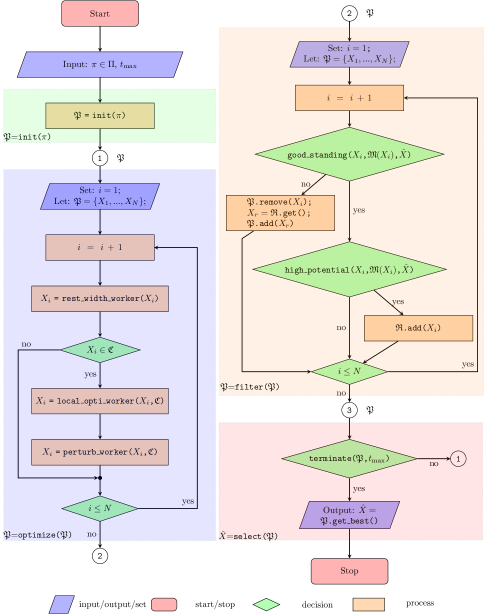
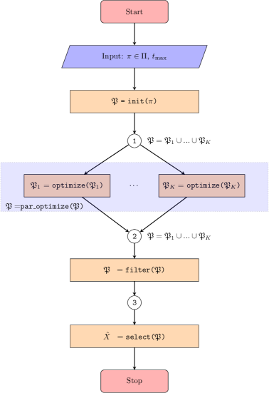
The details of the (SLS) optimization algorithm are presented in Figure 2, and they will be explained progressively in the forthcoming sections.

Figure 2: Architecture of optimization algorithm.

3.1 Initialization (init)

The initialization phase discovers initial candidate solutions (i.e., assignments $X$ which satisfy the job-admissibility constraint). The benefit of discovering such candidate solutions is rather important since it may fasten significantly the following optimization phase. Furthermore, if there exist a large number of local optima (as it is often the case), the starting point may influence significantly the resulting performance. To this end, it is necessary that we consider alternative fitness functions for the generation of candidate solutions.

The goal of the initialization routine is to create an initial set of job-admissible assignments $X$, denoted $\mathfrak{P}$ (main pool) of bounded maximum size ($\left|\mathfrak{P}\right|_{\max}$). This pool of candidate solutions will then be used for optimization. The possibilities for designing such a routine are, in fact, open ended. Here, we would like to provide one general structure, the specifics of which are provided in Table 1.

function $\mathfrak{P}$ = init($\pi$) //assignment based on criterion of (5),(6) or (7) FOR (every item $i$ in $\mathcal{I}$ (descending order)) SET $f_{i}^{*}=-\infty$ FOR (every object $j$ in $\mathcal{J}$ (descending order))     IF ($y_{i}(X)>0$ and $r_{j}(X)>b_{i}$)      $X_{:j}=X_{:j}+e_{i}$; (assign item $i$ to object $j$)      IF ($f_{i}(X;j)>f_{i}^{*}$)       $f_{i}^{*}=f_{i}(X;j)$; (accept item $i$)      ELSE       $X_{:j}=X_{:j}-e_{i}$; (remove item $i$)      END IF     END IF END FOR END FOR //populate main pool of candidate solutions SET $\mathfrak{P}$ = (multiple copies of) $X$

Table 1: init

As a first step, we sort both items $\mathcal{I}$ and objects $\mathcal{J}$ in descending order with respect to their width, similarly to a standard First-Fit-Decreasing (FFD) algorithm [37]. This is usually necessary, at least in cutting-stock problems, since large items may only fit in large objects. Then, for each item $i$ (with positive rest weight), we go through each available object $j$ (which may fit $i$), and we check whether an assignment of $i$ to $j$ maximizes a fitness criterion. In particular, we introduce here three candidate fitness functions:

1. negative weight of residual band of object $j$, i.e.,

   $$f_{i}(X;j)\doteq-r_{j}(X)\alpha_{j}.$$ (5)

   This fitness function is maximized when the weight of the residual band takes values that are close to zero. In other words, we try to fit as many objects as possible in each object $j\in\mathcal{J}$.

2. negative absolute rest weight of item $i$ minus the weight of the residual band of object $j\in\mathcal{J}$, i.e.,

   $$f_{i}(X;j)\doteq-|y_{i}(X)|-r_{j}(X)\alpha_{j}.$$ (6)

   Note that this function takes large values when both a) the rest weight of item $i$ and b) the residual weight of object $j$ are close to zero. In other words, under this criterion, we try to fit as many items as possible within object $j$ without though generating large rest weight for the selected items.

3. band $i$’s weight minus the weight of object $j$’s residual band, i.e.,

   $$f_{i}(X;j)\doteq\alpha_{j}b_{i}-\alpha_{j}r_{j}(X).$$ (7)

   Note that this function takes large values when the weight of item $i$ is large compared to the residual band’s weight, i.e., we try to fit as many bands as possible in each single object $j$.

Alternative fitness functions may be defined. Note that all the above fitness criteria employ a form of weight optimization (contrary to standard First-Fit-Decreasing algorithms). Such form of weight optimization is motivated primarily by two practical reasons: a) the difficulty in finding admissible assignments when the stock material is limited (something that cannot be guaranteed by standard First-Fit-Decreasing algorithms), and b) the limited time offered to solve the optimization problem, which makes the initial assignment a rather important factor over the final performance. In the forthcoming experimental evaluation (Section 6), we will demonstrate the impact of this good head-start in the final performance.

In the remainder of this paper, we will assume that an initial candidate solution $X$ that satisfies the job-admissibility constraint is available as a result of this initialization phase. Note that we do not impose the rest-width constraint during this initialization phase, due to the fact that in several cases it is rather difficult to meet this constraint. A special treatment of the rest-width constraint is suggested as part of the following optimization phase.

3.2 Optimization (optimize)

As described in Figure 2, the results of the init routine are used to populate an initial set of candidate solutions (main pool $\mathfrak{P}$) that will later be processed with optimize to generate admissible solutions for the optimization instance $\pi\in\Pi$.

In particular, the following steps are executed. First, the available candidate solutions in $\mathfrak{P}$ are sequentially processed through a sequence of working units. They are responsible for performing the necessary steps for either establishing admissible solutions and/or for further improving the performance of a candidate solution. We introduce three types of working units, namely:

• rest_width_worker($X$,$\mathfrak{C}$)

• local_opti_worker($X$,$\mathfrak{C}$)

• perturb_worker($X$,$\mathfrak{C}$)

where $\mathfrak{C}\doteq\{\mathcal{C}_{\rm job},\mathcal{C}_{\rm rw}\}$ is the family of constraints considered, corresponding to the job-admissibility (4b) and rest-width (4c) constraints.

The role of the rest_width_worker($X$,$\mathfrak{C}$) is to address the rest-width admissibility constraint, since it might not easily be satisfied for the job-admissible assignments generated at init. In case additional constraints were considered in the optimization problem (4), then additional such workers would have to be introduced.

The role of the local_opt_worker($X$,$\mathfrak{C}$) is to generate improved assignments $X$ with respect to the objective function in (4).

Finally, the role of the perturb_worker($X$,$\mathfrak{C}$) is to perform a sequence of perturbations in the currently admissible solutions in order to avoid convergence to local optima.

All these classes of working/processing units are based upon appropriately introduced modifications of the candidate solution $X$, so that either a constraint is satisfied or an improvement is observed in the cost function. These modifications, namely operations, constitute the core of the proposed optimization scheme and will be described in detail in the forthcoming Section 4. A set of available operations will be considered, denoted $\mathcal{O}$. Let also $o\in\mathcal{O}$ denote a representative element of this set. For now, we will only assume that each operation $o\in\mathcal{O}$ is equipped with three alternative modes, denoted:

• better_reply($X$,$\mathfrak{C}$,$g()$),

• constr_reply($X$,$\mathfrak{C}$,$\mathcal{B}$),

• random_reply($X$,$\mathfrak{C}$).

The above introduced modes designate three alternative possibilities for searching and executing operations in the candidate solution $X$. The better reply of an operation $o\in\mathcal{O}$, denoted better_reply($X$,$\mathfrak{C}$,$g()$), is based upon a semi-stochastic search of neighboring assignments to $X$ which improves the cost of the current assignment $X$, i.e., it generates an improved candidate solution with respect to the objective $g()$ that also satisfies the constraints in $\mathfrak{C}$. The constr_reply($X$,$\mathfrak{C}$,$\mathcal{B}$) mode performs a similar type of search, however the objective is to guarantee that the resulting assignment satisfies the constraints within $\mathfrak{C}$ of the optimization. The set $\mathcal{B}\subset\mathcal{J}$ is the set of “bad” objects that currently do not satisfy the constraint. Such a mode may be particularly beneficial when $X$ does not currently satisfy some of the constraints. Finally, the random_reply($X$,$\mathfrak{C}$) mode of an operation $o\in\mathcal{O}$ is based upon a random generation of local to $X$ assignments that satisfy the constraints $\mathfrak{C}$, however they may not necessarily improve the cost of $X$.

In the remainder of this section, we describe in detail the three introduced working units of the optimization routine which utilize some or all of the three alternative operation modes stated above.

Rest-width worker (rest_width_worker)

Note that the initially generated assignments $X$ in $\mathfrak{P}$ define candidate solutions that satisfy only the job-admissibility constraint (4b). The role of the rest-width worker is to operate on the candidate solutions on the main pool $\mathfrak{P}$, so that they satisfy the rest-width admissibility constraint for all objects $j\in\mathcal{J}$, without violating the job-admissibility constraint. The rest-width constraint is usually the most difficult constraint to be satisfied, and this is the reason it cannot be treated during the initialization phase of Section 3.1. Usually, a sequence of operations might be necessary before rest-width admissibility is achieved.

The rest-width worker is governed by the parameter $N_{\rm con}$ which corresponds to the total number of processing steps executed per each run of this worker. The architecture of the rest-width worker is presented in Table 2.

function $X$ = rest_width_worker($X$,$\mathfrak{C}$) REPEAT (for $N_{\rm con}$ times) SET $\mathcal{B}=\{j\in\mathcal{J}\mbox{ such that }r_{j}(X)\notin\mathcal{R}_{j}\}$ (find “bad” objects) IF ($\mathcal{B}=\varnothing$) (if there are no “bad” objects)     RETURN $X$ (return current assignment) ELSE (if there are “bad” objects)     FOR (oper=0 to oper<$\left|\mathcal{O}\right|$) (for each operation in $\mathcal{O}$)      SET $\mathcal{B}=\{j\in\mathcal{J}\mbox{ such that }r_{j}(X)\notin\mathcal{R}_{j}\}$ (find “bad” objects)      IF ($\mathcal{B}=\varnothing$)       RETURN $X$      ELSE       $X=\mathcal{O}$[oper].constr_reply($X$,$\mathfrak{C}$,$\mathcal{B}$) (execute constr_reply mode)      END IF     END FOR END IF END REPEAT

Table 2: rest_width_worker

As we can see, it simply executes a number of operations under the constr_reply mode until a rest-width admissible solution is found.

It is important to point out that if a candidate solution $X$ satisfies this constraint (after passing through this worker), then it will satisfy this constraint for the remaining of its processing history, i.e., no further processing will be requested for $X$ within this working unit. This is due to the fact that any subsequent working unit will never violate any of the constraints in $\mathfrak{C}$.

Local optimization worker (local_opt_worker)

The local optimization worker receives a candidate solution, $X$, which satisfies both constraints (4b)–(4c), i.e., job-admissibility and rest-width constraint. The objective is to perform local operations in the candidate solution $X$ under the better_reply mode, so that the resulting assignment reduces the cost (3), while maintaining admissibility.

The operation of the local-optimization worker is governed by $N_{\rm loc}\in\mathbb{N}$ which is the total number of operations executed per run of this worker. A description of this worker is provided in Table 3. Note that the number of steps executed within this worker is fixed and independent on whether a cost reduction is found or not.

function $X$ = local_opti_worker($X$,$\mathfrak{C}$) REPEAT (for $N_{\rm loc}$ times) RAND SET oper from {1,2,...,|$\mathcal{O}$|} $X=\mathcal{O}$[oper].better_reply($X$,$\mathfrak{C}$) END REPEAT

Table 3: local_opti_worker

Perturbation worker (perturb_worker)

With probability $\lambda>0$, a number of operations under the random_reply mode are executed while maintaining admissibility and without necessarily reducing the cost (3). A fixed number of $N_{\rm per}$ operations is executed per each run of this worker. The goal of such operations is to escape from local optima by temporarily accepting worse performances. A description of the architecture of the perturbation worker is provided in Table 4.

function $X$ = perturb_worker($X$,$\mathfrak{C}$) RAND SET t in [0,1] IF ( t < $\lambda$ ) REPEAT (for $N_{\rm per}$ times)     RAND SET oper from {0,1,...,$\left|\mathcal{O}\right|$}     $X=\mathcal{O}$[oper].random_reply($X$,{$\mathfrak{C}_{\rm job}$,$\mathfrak{C}_{\rm rw}$}) END REPEAT END IF

Table 4: perturb_worker

3.3 Filtering (filter)

The role of the filter is to assess the quality of the produced candidate solutions and to decide which of the candidate solutions need to be reprocessed and which should be reserved for later use.

The operation of the filter is based upon the notions of reprocessing and reservation. In particular, the filter is responsible for updating two sets of candidate solutions, namely the main pool $\mathfrak{P}$ and the reserve pool $\mathfrak{R}$. The pool, $\mathfrak{P}$, is the set of candidate solutions that are currently getting processed (i.e., they go through the optimization steps in optimize). The reserve pool, $\mathfrak{R}$, maintains candidate solutions from earlier stages of the optimization of high potential that may replace candidate solutions within the main pool $\mathfrak{P}$ upon request.

More specifically, the main steps of the filter are shown in Figure 2. In words, for each candidate solution $X_{i}$ of the main pool $\mathfrak{P}$, we first assess its good standing and decide on whether it should further be processed based on prior performances summarized in memory $\mathfrak{M}(X_{i})$. In particular, if $X_{i}$ is not of a good standing, then it is removed from the main pool (i.e., $\mathfrak{P}$.remove($X_{i}$)) and replaced by another candidate solution from the reserve pool (i.e., $X_{r}=\mathfrak{R}$.get() and $\mathfrak{P}$.add($X_{r}$)). If, instead, $X_{i}$ is of a good standing, then it remains part of the main pool $\mathfrak{P}$ and continues on the assessment of its high potential, based again on prior performances summarized in memory $\mathfrak{M}(X_{i})$. If $X_{i}$ is identified as having high potential, then it is saved into the reserve pool $\mathfrak{R}$ (i.e., $\mathfrak{R}$.add($X_{i}$)). When all candidate solutions have been filtered (i.e., assessed with respect to their good standing and high potential), then the main pool $\mathfrak{P}$ exits the filter.

The reserve pool $\mathfrak{R}$ is initially empty and it is gradually populated by solutions of high-potential. However, we assume that $\mathfrak{R}$ has a bounded maximum size $\left|\mathfrak{R}\right|_{\max}$, which means that when its capacity is reached, the newly entered solution will replace the oldest one in the pool. The reason for selecting a bounded maximum size is to allow for dynamic restarts within a bounded fitness-distance from the current best. In many practical scenarios, performing dynamic restarts from very early stages may delay significantly the optimization speed. However, by properly selecting the maximum size of the reserve pool, we may find an appropriate balance between earlier dynamic restarts and optimization speed.

It is also important to note that the maximum size of the main pool $\mathfrak{P}$ is also bounded by $\left|\mathfrak{P}\right|_{\max}$ (as discussed in Section 3.1). When a reserved solution needs to replace another one from the main pool, the oldest one in $\mathfrak{R}$ is always picked. Also, when a reserved solution is requested to replace $X\in\mathfrak{P}$ but $\mathfrak{R}$ is currently empty, then a replacement is not possible and the size of the main pool is going to reduce by one. When the main pool $\mathfrak{P}$ becomes empty, then the optimization should terminate.

Good standing (good_standing)

The function good_standing assesses the potential of a candidate solution $X$ to continue providing reductions in the cost value. It depends on the current version of the candidate solution $X$, its prior memory $\mathfrak{M}(X)$, and the currently best candidate solution $\hat{X}$. Informally, the role of the good-standing assessment is to capture whether a candidate solution $X$ is currently able to follow the path of the currently best candidate $\hat{X}$, and this is achieved by evaluating a) the fitness-distance of $X$ from the current best $\hat{X}$, b) the steps elapsed since the last time $X$ provided an improvement to $\hat{X}$, and c) the gradient of the cost reduction during the most recent processing steps of $X$. In fact, we would like that the candidate solution $X$ is sufficiently close to the current best, and its cost gradient is sufficiently large.

To accomplish this assessment, we first introduce the following parameters:

• $N_{\rm gs}^{*}$ denotes the number of processing steps over which the good standing of a candidate solution is evaluated.

• $D(X,\hat{X})$ denotes the normalized fitness-distance between $X$ and the current best $\hat{X}$, defined as follows:

  $$D(X,\hat{X})\doteq\frac{g(X)-g(\hat{X})}{g(\hat{X})}.$$

• $D_{\rm gs}^{*}$ denotes the maximum allowed normalized fitness distance from the current best for which the good standing is maintained.

• $G(X,\mathfrak{M}(X),N_{\rm gs}^{*})$ denotes the gradient of cost reduction observed in the candidate solution $X$, defined as follows:

  $$G(X,\mathfrak{M}(X),N_{\rm gs}^{*})\doteq\frac{g(X[N_{\rm ps}-N_{\rm gs}^{*}])-g(X[N_{\rm ps}])}{N_{\rm gs}^{*}\cdot g(X[N_{\rm ps}-N_{\rm gs}^{*}])}\geq 0,$$

  for $N_{\rm ps}>N_{\rm gs}^{*}$, where $N_{\rm gs}^{*}$ denotes the number of recent processing steps over which we estimate the gradient change of the cost function.

• $G_{\rm gs}^{*}$ denotes a threshold based on which the gradient $G$ of cost reduction is being evaluated.

• $N_{\rm rb}(X)$ denotes the number of processing steps since the candidate solution path leading to $X$ has provided a recent best (i.e., a reduction to the cost function).

In particular, the exact steps for assessing the good standing of $X$ are provided in Table 5.

function BOOL good_standing($X$,$\mathfrak{M}(X)$,$\hat{X}$) IF ( $N_{\rm ps}(X)$ > $N_{\rm gs}^{*}$) (if enough processing steps) IF ($D(X,\hat{X})$ < $D_{\rm gs}^{*}$ and $N_{\rm rb}(X)$ < $N_{\rm gs}^{*}$) (if $X$ is “close” to current best and recently provided an improvement)     IF ($G(X,\mathfrak{M}(X))$ > $G_{\rm gs}^{*}$) (if progress rate is large)      RETURN TRUE     ELSE (if progress rate is small)      RETURN FALSE     END IF ELSE (if $X$ is “far” from current best or recently provided no improvement)     RETURN FALSE END IF ELSE (if not enough processing steps yet) RETURN TRUE (good standing at early stages) END IF

Table 5: good_standing

First, we check whether enough processing steps have elapsed for the good standing criterion to be evaluated (i.e., $N_{\rm ps}(X)\geq N_{\rm gs}^{*}$). This initial check is required due to the absence of any prior knowledge regarding the potential of a candidate solution $X$. Then, we evaluate a) the normalized fitness-distance of $X$ from the current best $\hat{X}$, $D(X,\hat{X})$, and b) the processing steps elapsed since the last improvement offered by $X$, $N_{\rm rb}(X)$. Both have to be small enough to maintain a good standing. Lastly, we check whether $X$ exhibits a sufficiently large progress rate. If its progress rate is larger than $G_{\rm gs}^{*}$, then $X$ will retain its good standing. In other words, for maintaining a good standing, it is not sufficient that $X$ is close enough (with respect to fitness) to the current best, rather it should also provide a progress rate that is promising for improving the current best.

The parameters $D_{\rm gs}^{*}$, $G^{*}$, and $N_{\rm gs}^{*}$ need to be determined by the user.

High potential (high_potential)

The notion of high potential of a candidate solution $X$ captures its ability to provide significant reductions to the objective function (3). For example, an indicative criterion of a high potential is an extremely high progress rate $G(X,\mathfrak{M}(X))$. We wish to store candidate solutions exhibiting high potential at different stages of their processing paths, so that we are able to restart the processing from these stages. This form of restarts may serve as a mechanism for escaping from local optima, while at the same time it may increase the probability of converging to the optimal solution.

To assess the high potential of a candidate solution, we first introduce the following notation:

• $N_{\rm hp}^{*}$ denotes the number of processing steps over which the high potential of a candidate solution is evaluated.

• $D_{\rm hp}^{*}$ denotes the maximum allowed normalized fitness-distance from the current best for which the high potential property can be assessed.

• $G_{\rm hp}^{*}$ denotes a threshold based on which the gradient of cost reduction $G$ is being evaluated.

• $N_{\rm lr}(X)$ denotes the elapsed processing steps since the candidate solution $X$ was last reserved into $\mathfrak{R}$.

The exact steps for assessing the high potential of a candidate solution $X$ are provided in Table 6. First we check whether enough processing steps have elapsed for the high-potential criterion to be evaluated. Then, we evaluate a) the normalized fitness-distance of $X$ from the current best $\hat{X}$, $D(X,\hat{X})$, and b) the processing steps elapsed since the last reservation offered by the processing path of $X$. We would like $X$ to be close enough to the current best, however we would also like $X$ not to have provided recently any reservations (thus not creating subsequent reservations from the same processing paths). Lastly, we check whether $X$ exhibits a sufficiently large progress rate, i.e., larger than $G_{\rm hp}^{*}$.

function BOOL high_potential($X$,$\mathfrak{M}(X)$,$\hat{X}$) IF ( $N_{\rm ps}(X)$ > $N_{\rm hp}^{*}$ ) (if enough processing steps) IF ($D(X,\hat{X})$ < $D_{\rm hp}^{*}$ and $N_{\rm lr}(X)$ > $N_{\rm hp}^{*}$) (if $X$ is “close” to current best and has not recently been reserved)     IF ($G(X,\mathfrak{M}(X))$ > $G_{\rm hp}^{*}$) (if progress rate is large)      RETURN TRUE     ELSE (if progress rate is small)      RETURN FALSE     END IF ELSE (if $X$ is “far” from current best or it has recently been reserved)     RETURN FALSE END IF ELSE (if not enough processing steps) RETURN TRUE (assume high potential at early stages) END IF

Table 6: high_potential

We should expect that $D_{\rm gs}^{*}>D_{\rm hp}^{*}$ and that $G_{\rm gs}^{*}<G_{\rm hp}^{*}$, since high-potential should also imply good-standing but not the other way around.

3.4 Selection (select)

The last part of the optimization algorithm is the selection phase (select). In this phase, the main pool $\mathfrak{P}$ of candidate solutions has already been filtered, and the question is whether we should terminate processing and select the current best estimate $\hat{X}$ or continue processing $\mathfrak{P}$. The specifics of this phase are shown in Figure 2. The terminate decision is taken upon the current size of the main pool $\mathfrak{P}$ as well as the maximum allowed processing time $t_{\max}$ imposed by the user. In particular, when the size of the main pool is zero, or when the elapsed processing time has exceeded $t_{\max}$, then the optimization is terminated and the current best estimate $\hat{X}$ is provided as an output.

4 Operations

As we mentioned in the description of the optimization phase (optimize), the means by which local modifications of candidate solutions are created/searched is through a set of available operations $\mathcal{O}$. In this section, we would like to provide a description of the operations considered, as well as a description of their alternative modes (as initially introduced in Section 3.2), namely better_reply, constr_reply and random_reply.

The operations implemented are the following:

• MoveItem,

• SwapItems,

• SplitItem,

• RemoveObject,

• ReverseRemoveObject,

• RemoveItem,

4.1 MoveItem operation

Figure 3: MoveItem operation.

The move operation moves a single item from one object (or roll) to another object (see Figure 3). The details of the better_reply mode of this operation are described in Table 7.

function $X=$ MoveItem.better_reply($X$,$\mathfrak{C}$,$g()$) SET used_objects = get_used_objects($X$); REPEAT (for $N_{\rm br\_trials}$ times)    RAND SET object1 from used_objects    FOR (each item of object1)     REPEAT (for $N_{\rm br\_trials}$ times)      RAND SET object2 from all objects but object1      $X^{\prime}$ = $X$:move item from object1 to object2     IF ($X^{\prime}$ is $\mathfrak{C}$-admissible and $g(X^{\prime})$ < $g(X)$) }320pt[better reply]      SET $X$ = $X^{\prime}$ and RETURN $X$     END IF     END FOR    END FOR END REPEAT RETURN $X$

Table 7: MoveItem.better_reply

Note that this mode implements a form of nested search over the source object (object1), an item from this object (item) and the destination object (object2). Then, it operates a move of the item from object1 to object2. The object1 should be selected from the set of objects that are currently used (used_objects), i.e., from the set of objects with at least one item assigned to them. Given that the number of objects might be large, we can bound the size of this nested search via the parameter $N_{\rm br\_trials}$. The selection of this parameter depends on the number of available objects $\mathcal{J}$, and the desired time of optimization $t_{\max}$ determined by the user.

Similar in architecture is the constr_reply mode of this operation, however the objective is to simply generate admissible assignments for those objects that do not satisfy the constraint. The details are shown in Table 8.

function $X=$ MoveItem.constr_reply($X$,{$\mathcal{C}_{\rm job},\mathcal{C}_{\rm rw}$},$\mathcal{B}$) REPEAT ($N_{\rm con\_trials}$ times)    RAND SET bad_object from $\mathcal{B}$    FOR (each item of bad_object)     REPEAT ($N_{\rm con\_trials}$ times)      RAND SET object2 from all objects but bad_object      $X^{\prime}$ = $X$:move item from bad_object to object2     IF (item is $\mathcal{C}_{\rm job}$-admissible and bad_object is $\mathcal{C}_{\rm rw}$-admissible)      SET $X$ = $X^{\prime}$ and RETURN $X$     END IF     END REPEAT    END FOR END REPEAT RETURN $X$

Table 8: MoveItem.constr_reply

In particular, for $N_{\rm con\_trials}$ times, we go through the set of “bad” objects that do not satisfy the constraint. For each one of the items of this object, we go through a number of destination objects (different than the “bad” object), and we check whether admissibility of the modified assignment has been resolved with respect to the “bad” object (without violating the job-admissibility requirements for the moved item). Similarly to the better_reply mode, this mode is controlled by appropriately selecting the parameter $N_{\rm con\_trials}$.

The random_reply mode of this operation is described in Table 9.

function $X=$ MoveItem.random_init($X$,$\mathfrak{C}$) SET used_objects = get_used_objects($X$); REPEAT (for $N_{\rm rand\_trials}$ times)    RAND SET object1 from used_objects    RAND SET object2 from used_objects    IF (object1 is not equal to object2)     RAND SET item from the items of object1     $X^{\prime}$ = $X$:move item from object1 to object2     IF ($X^{\prime}$ is $\mathfrak{C}$-admissible) }320pt[$\mathfrak{C}$-admissibility]      SET $X$ = $X^{\prime}$ and RETURN $X$     END IF    END IF END REPEAT RETURN $X$

Table 9: MoveItem.random_init

It simply relies on a random selection of two (distinct) objects, one of which should have a non-zero number of items assigned to it. Then, an item is randomly picked from one of the objects and is assigned to the second object. The objective is to generate a new assignment $X^{\prime}$ that maintains $\mathfrak{C}$-admissibility. The effect of this mode into the cost is not considered.

Finally, note that there is not a unique way to initialize the objects/items involved in these modes, and this is also true for all the operations that follow. For example, in better_reply mode, we have selected a nested type of search to initialize the objects/items involved, while in random_reply mode, we implement a completely random initialization. This is not restrictive. In practice, a nested type of initialization of the parameters provided a faster discovery of better replies, however formulating the most efficient architecture for these modes requires a separate investigation.

4.2 SwapItems operation

Figure 4: SwapItems operation.

The SwapItems operation swaps one or more items from one object (or roll) with one or more items from another object (see Figure 4).

In particular, the SwapItems operation is based upon the selection of two objects (among all objects with non-zero items) and the selection of a combination of items from these objects. Then, the selected items from both objects are swapped with each other. Figure 4 provides an example, where two items from object $1$ are swapped with one item from object $2$.

The better_reply mode of this operation, for the case of 2 objects, is described in Table 7.

function $X=$ SwapItems.better_reply($X$,$\mathfrak{C}$,$g()$) SET used_objects = objects with non-zero items in $X$ REPEAT (for $N_{\rm br\_trials}$ times) RAND SET object1 from used_objects FOR (each combination comb1 of items in object1)     REPEAT (for $N_{\rm br\_trials}$ times)      RAND SET object2 from used_objects but object1      FOR (each combination comb2 of items in object2)       $X^{\prime}$ = $X$: swap all items in comb1 with all items in comb2      IF ($X^{\prime}$ is $\mathfrak{C}$-admissible and $g(X^{\prime})$ < $g(X)$) }320pt[better reply]       SET $X$ = $X^{\prime}$ and RETURN $X$      END IF     END REPEAT END FOR END REPEAT RETURN $X$

Table 10: SwapItems.better_reply

This mode incorporates the swap of a combination of items from object $1$ with another combination of items from object $2$ (different than object $1$). This mode can be augmented by alternative swap types, where more objects are involved.

The constr_reply and random_reply modes of the SwapItems operation are similar to the corresponding modes of the MoveItem operation, however following the structure of the swap operation. Accordingly, the random_reply mode is based upon a random selection of objects, and a random selection of a combination of items from these objects.

4.3 SplitItem operation

Figure 5: SplitItem operation.

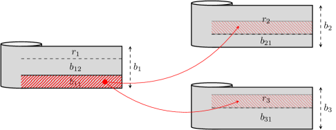
The SplitItem operation splits one item currently allocated in one object into two other distinct objects (see Figure 5).

The better_reply mode of this operation is described in Table 11.

function $X=$ SplitItem.better_reply($X$,$\mathfrak{C}$,$g()$) SET used_objects = objects with non-zero items in $X$ SET combs_objects = all combinations of 2 distinct objects out of $\mathcal{I}$ REPEAT (for $N_{\rm br\_trials}$ times) RAND SET object1 from used_objects REPEAT (for $N_{\rm br\_trials}$ times)     RAND SET a combination {object2,object3} from combs_objects     IF (object1 does not coincide with either object2 or object3)      FOR (each item in object1)       $X^{\prime}$ = $X$: split item to object2 and object3      IF ($X^{\prime}$ is $\mathfrak{C}$-admissible and $g(X^{\prime})$ < $g(X)$) }320pt[better reply]       SET $X$ = $X^{\prime}$ and RETURN $X$      END IF      END FOR     END IF END REPEAT END REPEAT RETURN $X$

Table 11: SplitItem.better_reply

This mode randomly selects an object (object1) from the set of used_objects and a combination of 2 distinct objects (object2 and object3) that are different from object1. Then it assigns a randomly selected item from object1 to both object2 and object3. This selection of objects and an item is repeated for a fixed number of times controlled by $N_{\rm br\_trials}$ or until a better reply is found.

The constr_reply and random_reply modes of the SplitItem operation are similar to the random mode of the MoveItem operation, however following the structure of the SplitItem operation.

4.4 RemoveObject operation

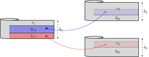
The RemoveObject operation involves an object with two or more items and moves a combination of its items to new distinct objects (which may or may not have items assigned to them), see Figure 6. In a way, the RemoveObject operation compliments the MoveItem operation, since it involves more than one item and more than one destination objects.

Figure 6: RemoveObject operation.

The better_reply mode of this operation is described in Table 12.

function $X=$ RemoveObject.better_reply($X$,$\mathfrak{C}$,$g()$) SET used_objects = all objects with at least 2 items in $X$ REPEAT (for $N_{\rm br\_trials}$ times) RAND SET object1 from used_objects REPEAT (for $N_{\rm br\_trials}$ times)     RAND SET comb as a combination of 2 or more items in object1     REPEAT (for $N_{\rm br\_trials}$ times)      RAND SET dest_objects as a combination of $\left|\mathtt{{\color[rgb]{.5,0,.5}\definecolor[named]{pgfstrokecolor}{rgb}{.5,0,.5}comb}}\right|$ objects in $\mathcal{J}$      FOR (each item j of comb)       $X^{\prime}$ = $X$: move item j from object1 to dest_objs[j]      IF ($X^{\prime}$ is $\mathfrak{C}$-admissible and $g(X^{\prime})$ < $g(X)$ }320pt[better reply]       SET $X$ = $X^{\prime}$ and RETURN $X$      END IF      END FOR     END REPEAT END REPEAT END REPEAT RETURN $X$

Table 12: RemoveObject.better_reply

According to this mode, we select a) a source object, b) a combination of items from the source object, and c) a combination of distinct destination objects equal in number to the selected items. Then, each one of the items moves to one of the destination objects, so that the cost of the optimization is reduced (e.g., see example of Figure 6).

Similarly, we may define the constr_reply and random_reply models of this operations (the same way we did for the MoveItem operation in Section 4.1).

4.5 ReverseRemoveObject operation

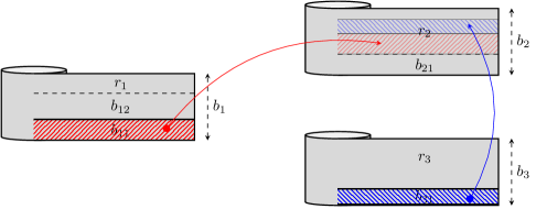
The ReverseRemoveObject operation performs a reverse form of the RemoveObject operation. In particular, the goal of this operation is to combine items from several source objects and move them into a new destination object, see Figure 7.

Figure 7: ReverseRemoveObject operation.

The better_reply mode of this operation is described in Table 13.

function $X=$ ReverseRemoveObject.better_reply($X$,$\mathfrak{C}$,$g()$) SET used_objects = all objects with non-zero items in $X$ REPEAT (for $N_{\rm br\_trials}$ times) RAND SET a combination comb of 2 objects in used_objects REPEAT (for $N_{\rm br\_trials}$ times)     RAND SET dest_object from all objects not in comb     SET $X^{\prime}$ = $X$     FOR (each source_object in comb)      RAND SET item from the items of source_object      $X^{\prime}$ = $X^{\prime}$: move item from source_object to dest_object     END FOR     IF ($X^{\prime}$ is $\mathfrak{C}$-admissible and $g(X^{\prime})$ < $g(X)$) }320pt[better reply]      SET $X$ = $X^{\prime}$ and RETURN $X$     END IF END REPEAT END REPEAT RETURN $X$

Table 13: ReverseRemoveObject.better_reply

According to this mode, we find a) a combination of source objects, b) an item from each source object, and c) a destination object. We, then, move the selected items to the destination object and we check whether the cost has been reduced.

The constr_reply and random_reply modes of this operation can be defined in a similar way, as we did for the MoveItem operation in Section 4.1.

4.6 RemoveItem operation

The RemoveItem operation checks whether an item assigned to an object can be removed without violating any of the constraints (i.e., job-admissibility and rest-width constraints). Obviously if any such item can be removed without violating the constraints, then it is likely that the objective function will be reduced. For example, this might be the case when there are objects with a single item assigned to them. The better_reply mode of this operation is described in Table 14.

function $X$ = RemoveItem.better_reply($X$,$\mathfrak{C}$,$g()$) SET used_objects = all objects with non-zero items in $X$ REPEAT (for $N_{\rm br\_trials}$ times) RAND SET object from used_objects FOR (each item of object)     $X^{\prime}$ = $X$: remove item from object IF ($X^{\prime}$ is $\mathfrak{C}$-admissible and $g(X^{\prime})$ < $g(X)$) }320pt[better reply]     SET $X$ = $X^{\prime}$ and RETURN $X$ END IF END FOR END REPEAT RETURN $X$

Table 14: RemoveItem.better_reply

Similar is the reasoning in constr_reply and random_reply modes of this operation.

5 Diversification Strategies

The proposed structure of the optimization algorithm may naturally incorporate several diversification strategies. Diversification strategies aim at preventing the search process getting trapped in local optima. In this section, we present a set of possible diversification strategies that can be exploited.

Given that optimization problems of the form (4) may differ significantly from each other, both in the number of feasible solutions as well as in the search space, the development of a unified selection and tuning of diversification strategies becomes almost impossible. The goal of this paper is to demonstrate that the diversification strategies considered here can make a difference at least on average.

We may group the set of diversification strategies considered here in the following categories.

• Diverse initialization strategies

• Bounded-distance dynamic restarts

• Random perturbations

• Parallelization

• Cost-free operations

5.1 Diverse initialization strategies

As we discussed in Section 3.1, we introduced three alternative criteria in the formulation of initial candidate solutions. Our objective is to generate initial admissible solutions that a) are close enough to the optimal solution, and b) are diverse enough to increase the possibility for convergence to the optimal solution.

5.2 Bounded-distance dynamic restarts

A candidate solution may currently be located at search spaces with no significant potential in reducing the current cost. Thus, in order to avoid stagnation, we allow such candidate solution to be replaced by another one from an earlier stage but within a bounded fitness distance from the current best. There are two operations that indirectly control the process of dynamic restarts, namely the good_standing and high_potential functions. As already described in Section 3.3, the good_standing function and its parameters (i.e., $D_{\rm gs}^{*}$, $G_{\rm gs}^{*}$ and $N_{\rm gs}^{*}$) control the criteria for dropping a candidate solution, while the high_potential function and its parameters (i.e., $D_{\rm hp}^{*}$, $G_{\rm hp}^{*}$ and $N_{\rm hp}^{*}$) control the criteria for reserving a candidate solution. Apart from these parameters, the size of the main and reserve pool also affect the evolution of the optimization algorithm. These parameters need to be carefully tuned so that the bounded-distance dynamic restarts increase the probability of escaping from a local optimum without though delaying significantly the optimization process. The response to these parameters may differ significantly between application scenarios.

5.3 Random perturbations

Random perturbations constitute an alternative way to avoid stagnation, through the introduction of a sequence of randomly generated operations. In particular, with a small positive probability $\lambda>0$, a candidate solution goes through the perturb_worker, in which a sequence of operations is randomly selected, and a random initialization of this operation is set (random_reply mode). If the perturbation leads to an admissible solution, then the modification is accepted independently of the resulting objective value. This is essentially similar in spirit with the random-walk extension introduced in [20].

5.4 Parallelization

The implementation of the optimization algorithm depicted in Figure 2 suggests a high-level (domain-specific) parallel architecture that does not fit to standard parallel patterns. Simple for-loop parallelization, using, e.g., a parallel-for pattern, is not possible, since the iteration space is not known a-priori. In fact, we do not know how many times a candidate solution should pass through the optimization worker (local_opt_worker) before we stop processing it.

To this end, first we partition the main pool $\mathfrak{P}$ into $K$ sets of candidate solutions (where $K$ is our planned parallel degree). We then process these sets in parallel through the optimize function. Finally, we decide on whether a candidate solution should continue processing through the implementation of the filter. The proposed parallelization architecture is depicted in Figure 8.

The proposed parallel pattern is a modification of the so-called pool-pattern, first implemented in [31] and incorporated in the FastFlow parallel programming framework in [2]. The modification lies in the introduction of the reserve pool $\mathfrak{R}$ that simplifies the implementation of the bounded-distance dynamic restarts, which is an essential part of several SLS algorithms.

As probably expected, the larger the parallel degree, the larger the probability of getting closer to the optimal solution. This will be demonstrated through experiments in the forthcoming Section 6, but it may also be supported by the statistical literature [28] as pointed out in [20].

Figure 8: Parallel architecture.

5.5 Cost-free operations

By cost-free operations we mean operations that may result in (practically) the same cost. The role of such operations may be proven rather important mainly because they introduce perturbations with no impact to the objective. Thus, through such operations, we may diversify the search of optimal solutions without necessarily restarting from worse assignments. More formally, let $X^{\prime}$ be a modification over an initial candidate solution $X$. A modification becomes acceptable subject to a better-reply criterion if the following smooth condition is satisfied:

$$g(X^{\prime})<g(X)+\zeta(X,X^{\prime}),$$ (8)

for some real-valued function $\zeta$. Function $\zeta$ applies a form of extra allowance in the acceptance of an improvement. For example, we may assume that $\zeta=\epsilon$ for some small positive constant $\epsilon>0$. Alternative criteria may be defined.

6 Experimental Evaluation

The goal in this section is to evaluate the behavior of the evolutionary algorithm and understand the role of the alternative diversification strategies introduced. In particular, we are going to demonstrate the effect of each one of the proposed diversification strategies in the overall performance of the algorithm. To this end, we consider a number of optimization problems of the form (4) borrowed from the industry of manufacturing transformer cores (cf., [8]). Each optimization problem is fully described by a set of available rolls and a set of required items to be produced (characterized by their width and weight). The optimization problems considered span from jobs of small number of items to medium or large number of items, thus covering a range of possibilities and enough variety to test the effect of the proposed algorithm and the diversification strategies.

The optimization problem (4) minimizes the used objects’ weight. Since the performance of the optimization might be affected by the size of the problem (i.e., the weight of the produced items), we introduce a performance metric normalized by the size of the problem. Let us assume that a set $\Pi$ of different optimization problems is considered. Let $\hat{X}_{\pi}$ denote the best estimate discovered by the algorithm, and $W_{\pi}$ be the total weight of the required items, i.e., $W_{\pi}\doteq\sum_{i\in\mathcal{I}}w_{i}$. We introduce the following evaluation metric, $\mathcal{G}:\Pi\to\mathbb{R}_{+}$, such that

$$\mathcal{G}(\pi)\doteq\frac{g(\hat{X}_{\pi})}{W_{\pi}}\frac{g(\hat{X}_{\pi})}{\sum_{\pi\in\Pi}g(\hat{X}_{\pi})}.$$ (9)

The first part of the performance metric corresponds to the ratio of objects’ weight over the items’ weight. Naturally the higher this ratio is, the less efficient the solution would be. However, an inefficient solution at a small-size problem does not have the same impact with an inefficient solution at a large-size problem. To this end, the role of the second ratio is to normalize the effect of the solution in the overall cost. Furthermore, note that $\sum_{\pi\in\Pi}\mathcal{G}(\pi)$ is the weighted average ratio of the used objects’ weight over the required items’ weight, i.e., it captures the efficiency of the optimization.

In the following subsections, we will investigate the effect of the alternative diversification strategies proposed here (as well as some of the optimization parameters) and their impact in the overall performance of the algorithm via metric (9).

Diverse initialization strategies

We start our investigation by varying the set of strategies considered in the initialization phase of the algorithm. In Figure 9, we see the impact of the initially considered candidate solutions when we restrict the set of strategies used to generate them. In the first scenario (dashed line), we employ the initialization criterion of Equation (5), while in the second scenario (solid line), we consider all available initialization criteria of Equations (5)–(7). In either case, the initial set of candidate solutions (main pool $\mathfrak{P}$) has the same size and it is populated equally by each one of the considered initialization strategies.

Figure 9: The effect of initialization strategies.

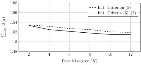
It is important to point out that the benefit of the larger variety of initialization strategies is also due to the fact that the considered strategies employ a form of weight optimization therein. We should not expect that the same improvement occurs when we consider initialization strategies that do not apply a form of weight optimization.

In Figure 9, as well as in the following experiments, we also demonstrate how the performance varies as we increase the parallel degree ($K$). This corresponds to the effect of parallelization following the architecture of Figure 8. Furthermore, in all these experiments, $t_{\max}=5min$, unless otherwise specified.

Random perturbations

In this set of experiments, we would like to test the effect of the random perturbations controlled by the parameter $\lambda>0$. Figure 10 shows the increase in performance when $\lambda$ increases to $\lambda=0.1$ (i.e., with probability $0.1$, a candidate solution goes through the perturb_worker.

Figure 10: The effect of random perturbations.

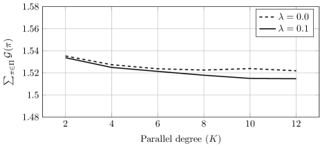
Note that the random perturbations have a positive impact in the optimization performance.

Optimization time

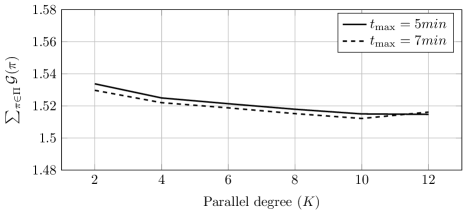
We would also like to investigate how the optimization algorithm responds when the maximum allowed optimization time ($t_{\max}$) increases. It is natural to expect that the performance in this case should increase, since some of the candidate solutions will be processed for a longer period of time. Note further that the increase in performance seems to reduce as we increase the parallel degree. One explanation for this behavior is the fact that an increased parallel degree already allows for a faster processing, thus it is highly likely that we are already sufficiently close to the optimal solution.

Figure 11: The effect of simulation time.

High-potential threshold

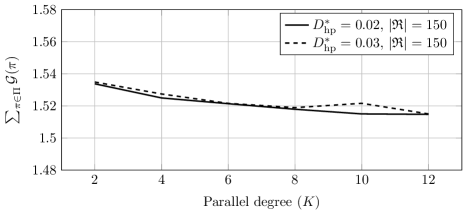
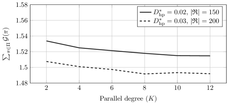
Recall that $D_{\rm hp}^{*}$ and $G_{\rm hp}^{*}$ are two thresholds that control the reservation of candidate solutions into the reserve pool $\mathfrak{R}$. We would like here to investigate the effect of $D_{\rm hp}^{*}$ which corresponds to the normalized fitness-distance from the current best within which a high-potential candidate solution can be stored into the reserve pool $\mathfrak{R}$. In other words, we would like to investigate how the performance of the optimization varies when we move the reservation threshold towards earlier stages.

When candidate solutions from earlier stages are stored into the reserve pool $\mathfrak{R}$, we should expect that the escape probability from local optima should increase. However, the size of the reserve pool $\mathfrak{R}$ is fixed, which means that the oldest candidate solutions may be dropped to create space for more recent reservations. Thus, when we just increase the threshold $D_{\rm hp}^{*}$ the benefit is not guaranteed (Figure 12). However, if we also increase the size of the reserve pool, then the benefit for increasing the threshold can be materialized (Figure 13).

Figure 12: The effect of high-potential threshold.

Figure 13: The effect of high-potential threshold as we increase the size of the reserve pool.

Good-standing threshold

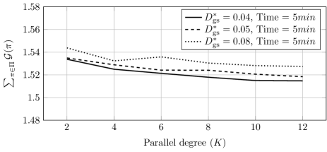
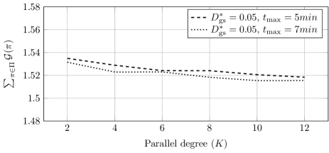
Recall that $D_{\rm gs}^{*}$ and $G_{\rm gs}^{*}$ are two thresholds that control the assessment over allowing a candidate solution to continue processing (Section 3.3). In particular, $D_{\rm gs}^{*}$ denotes the normalized fitness distance from the current best within which a candidate solution is allowed to continue processing. We wish to investigate how the performance of the optimization will change as we increase $D_{\rm gs}^{*}$, i.e., if we allow candidate solutions to remain longer within the main pool $\mathfrak{P}$.

Figure 14 demonstrates how the performance changes as we progressively increase $D_{\rm gs}^{*}$. As expected, the longer we allow a candidate solution to remain within the main pool, the slower the rate of using reserved candidate solutions, and the greater the probability that the process is trapped in a local optimum. Thus, we should expect that the performance may degrade as we increase $D_{\rm gs}^{*}$ more than necessary (Figure 14). However, if we also increase the optimization time, then we may achieve better performance (since we exploit better the fact that solutions remain in the pool for longer periods of time), Figure 15.

Figure 14: The effect of good-standing threshold.

Figure 15: The effect of the good-standing threshold.

Cost-free operations

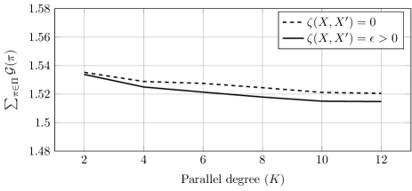
In the last experiment, we wish to investigate the effect of cost-free operations in the performance of the optimization. Cost-free operations essentially allow for local operations that do not have any significant impact in the overall performance. As probably expected, this allows for a candidate solution to escape from a local optimum with no impact in the performance. Figure 16 demonstrates the fact that cost-free operations can indeed increase the overall performance rather constantly over the parallel degree.

Figure 16: The effect of cost-free operations.

7 Conclusions

This paper presented an evolutionary SLS algorithm specifically tailored for one-dimensional cutting-stock optimization problems. The novelty of the proposed algorithm lies in its architecture that allowed for the introduction of a novel parallel pattern and the easy integration of a large family of diversification strategies. Although the proposed SLS algorithm was presented within the context of one-dimensional cutting-stock problems, its architecture is generic enough to be integrated into a larger family of combinatorial optimization problems. Finally, the presented experimental evaluation demonstrated a significant improvement in efficiency due to both the proposed parallel pattern as well as the additional diversification strategies presented.

References

- [1] Aktin, T., Özdemir, R.G.: An integrated approach to the one-dimensional cutting stock problem in coronary stent manufacturing. European Journal of Operational Research 196(2), 737–743 (2009)
- [2] Aldinucci, M., Campa, S., Danelutto, M., Kilpatrick, P., Torquati, M.: Pool Evolution: A Parallel Pattern for Evolutionary and Symbolic Computing. International Journal of Parallel Programming 44(3), 531–551 (Jun 2016)
- [3] Belov, G., Scheithauer, G.: A cutting plane algorithm for the one-dimensional cutting stock problem with multiple stock lengths. European Journal of Operational Research 141, 274–294 (2002)
- [4] Belov, G., Scheithauer, G.: A branch-and-cut-and-price algorithm for one-dimensional stock cutting and two-dimensional two-stage cutting. European Journal of Operational Research 171, 85–106 (2006)
- [5] Beraldi, P., Bruni, M.E., Conforti, D.: The stochastic trim-loss problem. European Journal of Operational Research 197(1), 42–49 (2009)
- [6] Brooks, R.L., Smith, C.A.B., Stone, A.H., Tutte, W.T.: The Dissection of Rectangles Into Squares, pp. 88–116. Birkhäuser Boston, Boston, MA (1987)
- [7] de Carvalho, J.V.: LP models for bin packing and cutting stock problems. European Journal of Operational Research 141, 253–273 (2002)
- [8] Chasparis, G., Zellinger, W., Haunschmid, V., Riedenbauer, M., Stumptner, R.: On the optimization of material usage in power transformer manufacturing. In: 2016 IEEE 8th International Conference on Intelligent Systems (IS). pp. 680–685 (Sep 2016)
- [9] Cherri, A.C., Arenales, M.N., Yanasse, H.H., Poldi, K.C., Gonçalves Vianna, A.C.: The one-dimensional cutting stock problem with usable leftovers - A survey. European Journal of Operational Research 236(2), 395–402 (Jul 2014)
- [10] Dyckhoff, H.: A typology of cutting and packing problems. European Journal of Operational Research 44, 145–159 (1990)
- [11] Gerstl, A., Karisch, S.E.: Cost optimization for the slitting of core laminations for power transformers. Annals of Operations Research 69, 157–169 (1997)
- [12] Gilmore, P., Gomory, R.: A linear programming approach to the cutting stock problem. Operations Research 9, 848–859 (1961)
- [13] Gilmore, P., Gomory, R.: A linear programming approach to the cutting stock problem, Part II. Operations Research 11, 863–888 (1963)
- [14] Gradišar, M., Kljajić, M., Resinović, G., Jesenko, J.: A sequential heuristic procedure for one-dimensional cutting. European Journal of Operational Research 114, 557–568 (1999)
- [15] Gradišar, M., Trkman, P.: A combined approach to the solution to the general one-dimensional cutting stock problem. Computers and Operations Research 32, 1793–1807 (2005)
- [16] Haessler, R.W., Sweeney, P.E.: Cutting stock problems and solution procedures. European Journal of Operational Research 54, 141–150 (1991)
- [17] Haouari, M., Serairi, M.: Heuristics for the variable sized bin-packing problem. Computers and Operations Research 36 (2009)
- [18] Hinterding, R., Khan, L.: Genetic algorithms for cutting stock problems: With and without contiguity. In: Selected Papers from the AI’93 and AI’94 Workshops on Evolutionary Computation, Process in Evolutionary Computation. pp. 166–186. AI 9́3/AI 9́4, Springer-Verlag, London, UK, UK (1995)
- [19] Holthaus, O.: Decomposition approaches for solving the integer one-dimensional cutting stock problem with different types of standard lengths. European Journal of Operational Research 141, 295–312 (2002)
- [20] Hoos, H., Stützle, T.: Stochastic Local Search: Foundations and Applications. Elsevier Inc. (2005)
- [21] Kallrath, J., Rebennack, S., Kallrath, J., Kusche, R.: Solving real-world cutting stock-problems in the paper industry: Mathematical approaches , experience and challenges. European Journal of Operational Research 238(1), 374–389 (2014)
- [22] Kantorovich, L.: Mathematical methods of organizing and planning production. Management Science 6, 366–422 (1960)
- [23] Lodi, A., Martello, S., Monaci, M.: Two-dimensional packing problems: A survey. European Journal of Operational Research 141(2), 241–252 (2002)
- [24] Lu, H.c., Huang, Y.h.: An efficient genetic algorithm with a corner space algorithm for a cutting stock problem in the TFT-LCD industry. European Journal of Operational Research 246(1), 51–65 (2015)
- [25] Onwubolu, G.C., Mutingi, M.: A genetic algorithm approach for the cutting stock problem. Journal of Intelligent Manufacturing 14, 209–218 (2003)
- [26] Pentico, D.W.: The assortment problem : A survey. European Journal of Operational Research 190, 295–309 (2008)
- [27] Péter, A., András, A., Zsuzsa, S.: A Genetic Solution for the Cutting Stock Problem (1996)
- [28] Rohatgi, V.: An Introduction to Probability Theory and Mathematical Statistics. John Wiley & Sons, New York, NY (1976)
- [29] Romanowski, A., Nowotniak, R., Kawecki, K., Jaworski, T., Chaniecki, Z., Grudzień, K.: Evolutionary Algorithms Approach for Cutting Stock Problem. Image Processing & Communications 17(4), 297–306 (2012)
- [30] Rossbory, M., Chasparis, G.: Parallelization of stochastic-local-search algorithms using high-level parallel patterns. In: High-Level Programming for Heterogeneous and Hierarchical Parallel Systems. Prague, Czech Republic (Jan 2016)
- [31] Rossbory, M., Reisner, W.: Parallelization of Algorithms for Linear Discrete Optimization Using ParaPhrase. In: 2013 24th International Workshop on Database and Expert Systems Applications. pp. 241–245 (Aug 2013)
- [32] Shahin, A.a., Salem, O.M.: Using genetic algorithms in solving the one-dimensional cutting stock problem in the construction industry. Canadian Journal of Civil Engineering 31, 321–332 (2004)
- [33] Shao, X., Li, X., Gao, L., Zhang, C.: Integration of process planning and scheduling - A modified genetic algorithm-based approach. Computers and Operation Research 36, 2082–2096 (2009)
- [34] Sweeney, P.E., Haessler, R.W.: One-dimensional cutting stock decisions for rolls with multiple quality grades. European Journal of Operational Research 44(June 1988), 224–231 (1990)
- [35] Umetani, S., Yagiura, M., Ibaraki, T.: One-dimensional cutting stock problem to minimize the number of different patterns. European Journal of Operational Research 146, 388–402 (2003)
- [36] Wäscher, G., Haußner, H., Schumann, H.: An improved typology of cutting and packing problems. European Journal of Operational Research 183, 1109–1130 (2007)
- [37] Williamson, D.P., Shmoys, D.B.: The Design of Approximation Algorithms. Cambridge University Press, New York, NY, USA, 1st edn. (2011)
- [38] Yanasse, H.H., Limeira, M.S.: A hybrid heuristic to reduce the number of different patterns in cutting stock problems. Computers and Operations Research 33, 2744–2756 (2006)