Algebraic Relations and Triangulation of Unlabeled Image Points

André Wagner Technische Universität Berlin
Berlin, Germany
http://page.math.tu-berlin.de/~wagner
(Date: July 2017)
Abstract.

In multiview geometry when correspondences among multiple views are unknown the image points can be understood as being unlabeled. This is a common problem in computer vision. We give a novel approach to handle such a situation by regarding unlabeled point configurations as points on the Chow variety Symm(2)subscriptSym𝑚superscript2\operatorname*{Sym}_{m}(\mathbb{P}^{2}). For two unlabeled points we design an algorithm that solves the triangulation problem with unknown correspondences. Further the unlabeled multiview variety Symm(VA)subscriptSym𝑚subscript𝑉𝐴\operatorname*{Sym}_{m}(V_{A}) is studied.

1. Introduction

In many computer vision applications, the correspondences among views are unknown. Hence the m𝑚m world points in 3superscript3\mathbb{P}^{3} and their images points in 2superscript2\mathbb{P}^{2} will be unlabeled. The multiview variety VAsubscript𝑉𝐴V_{A} [1] is a fundamental object in multiview geometry, it encodes the relations among n𝑛n image points of one world point in n𝑛n images taken by n𝑛n cameras. To study the problem of unlabeled data, we propose to work with the unlabeled multiview variety. This is the variety of products of multiview varieties [1] with unknown correspondences. An unlabeled point configuration in (2)msuperscriptsuperscript2𝑚(\mathbb{P}^{2})^{m} is a point in the Chow variety Symm(2)subscriptSym𝑚superscript2\operatorname*{Sym}_{m}(\mathbb{P}^{2}) [6, §8.6]. Algebraically the unlabeled multiview variety is the image of the multiview variety under the quotient map ((2)m)n(Symm(2))nsuperscriptsuperscriptsuperscript2𝑚𝑛superscriptsubscriptSym𝑚superscript2𝑛\bigl{(}(\mathbb{P}^{2})^{m}\bigr{)}^{n}\rightarrow\bigl{(}\operatorname*{Sym}_{m}(\mathbb{P}^{2})\bigr{)}^{n} for the symmetric group S(m)𝑆𝑚S(m) action. Our focus is mostly on two unlabeled points. We design Algorithm 2 to triangulate two unlabeled points.

While labeled world and image configurations are points in (2)msuperscriptsuperscript2𝑚(\mathbb{P}^{2})^{m} and (2)msuperscriptsuperscript2𝑚(\mathbb{P}^{2})^{m}, unlabeled image configurations are points in the Chow varieties which live as subvarieties in Symm(2)subscriptSym𝑚superscript2\operatorname*{Sym}_{m}(\mathbb{P}^{2}) and Symm(3)subscriptSym𝑚superscript3\operatorname*{Sym}_{m}(\mathbb{P}^{3}). This is the variety of ternary forms that are products of m𝑚m linear forms (cf. [6, §8.6]), respectively quaternary forms that are products of m𝑚m linear forms. It is embedded in the space (m+2m)1superscriptbinomial𝑚2𝑚1\mathbb{P}^{\binom{m+2}{m}-1} of all ternary forms of degree m𝑚m.

We start by giving a brief introduction to multiview geometry. A camera is a linear map from the three-dimensional projective space 3superscript3\mathbb{P}^{3} to the projective plane 2superscript2\mathbb{P}^{2}, both over \mathbb{R}. We represent n𝑛n cameras by matrices A1,A2,,An3×4subscript𝐴1subscript𝐴2subscript𝐴𝑛superscript34A_{1},A_{2},\ldots,A_{n}\in\mathbb{R}^{3\times 4} of rank 333. A world point X3𝑋superscript3X\in\mathbb{P}^{3} is mapped by the perspective relation of the camera Aj3×4subscript𝐴𝑗superscript34A_{j}\in\mathbb{R}^{3\times 4}

AjX=λjuj,λj{0}formulae-sequencesubscript𝐴𝑗𝑋subscript𝜆𝑗subscript𝑢𝑗subscript𝜆𝑗0A_{j}X=\lambda_{j}u_{j},\,\lambda_{j}\in\mathbb{R}\setminus\{0\}

to the image point uj2subscript𝑢𝑗superscript2u_{j}\in\mathbb{P}^{2}. The kernel of Ajsubscript𝐴𝑗A_{j} is the focal point fj3subscript𝑓𝑗superscript3f_{j}\in\mathbb{P}^{3}. Each image point uj=(uj0,uj1,uj2)2subscript𝑢𝑗subscript𝑢𝑗0subscript𝑢𝑗1subscript𝑢𝑗2superscript2u_{j}=(u_{j0},u_{j1},u_{j2})\in\mathbb{P}^{2} of camera Ajsubscript𝐴𝑗A_{j} has a line through fjsubscript𝑓𝑗f_{j} as its fiber in 3superscript3\mathbb{P}^{3}. This is the back-projected line. On that back-projected line lies the world point X3𝑋superscript3X\in\mathbb{P}^{3}. A camera is called normalized if it is of the form [I|c]delimited-[]conditional𝐼𝑐[I\,|\,c] form some vector c3𝑐superscript3c\in\mathbb{R}^{3}, with I3×3𝐼superscript33I\in\mathbb{R}^{3\times 3} being the identity matrix.

We assume throughout the paper that the focal points of the n𝑛n cameras are in general position, i.e. all distinct, no three on a line, and no four on a plane. Let βjksubscript𝛽𝑗𝑘\beta_{jk} denote the line in 3superscript3\mathbb{P}^{3} spanned by the focal points fjsubscript𝑓𝑗f_{j} and fksubscript𝑓𝑘f_{k}. This is the baseline of the camera pair Aj,Aksubscript𝐴𝑗subscript𝐴𝑘A_{j},A_{k}. The image of the focal point fjsubscript𝑓𝑗f_{j} in the k𝑘kth-image plane of the camera Aksubscript𝐴𝑘A_{k} is the epipole ekjsubscript𝑒𝑘𝑗e_{kj}.

For three cameras Aj,Ak,Alsubscript𝐴𝑗subscript𝐴𝑘subscript𝐴𝑙A_{j},A_{k},A_{l} the plane spanned by their focal points is called trifocal plane.

Computing the point of intersection of the back-projected lines to reconstruct X𝑋X is called triangulation[4, §9.1]. The triangulation can be based on multiple views and amounts to solve the linear equations

(1) B[Xλ1λn]= 0whereB=[A1u100A20u20An00un]3n×(4+n).formulae-sequence𝐵matrix𝑋subscript𝜆1subscript𝜆𝑛 0where𝐵matrixsubscript𝐴1subscript𝑢100subscript𝐴20subscript𝑢20subscript𝐴𝑛00subscript𝑢𝑛superscript3𝑛4𝑛\quad B\begin{bmatrix}\,X\\ -\lambda_{1}\\ \vdots\\ -\lambda_{n}\end{bmatrix}\,=\,0\qquad\hbox{where}\quad B\,=\,\begin{bmatrix}A_{1}&u_{1}&0&\ldots&0\\ A_{2}&0&u_{2}&\ddots&0\\ \vdots&\vdots&\ddots&\ddots&\vdots\\ A_{n}&0&\ldots&0&u_{n}\end{bmatrix}\,\in\,\mathbb{R}^{3n\times(4+n)}.

For generic data the world point X𝑋X is represented by the first four entries of any element in the kernel of B𝐵B. In practice this equation system is solved by a singular value decomposition and similar approaches [3]. Such that a reconstruction of X𝑋X restricted to only two views is possible the image points must satisfy a bilinear relation

ukTFuj=0,with F3×3.formulae-sequencesuperscriptsubscript𝑢𝑘𝑇𝐹subscript𝑢𝑗0with 𝐹superscript33u_{k}^{T}Fu_{j}=0,\,\text{with }F\in\mathbb{R}^{3\times 3}.

The matrix F𝐹F is called fundamental matrix of views j𝑗j and k𝑘k.

The multiview variety VAsubscript𝑉𝐴V_{A} of the camera configuration A=(A1,,An)𝐴subscript𝐴1subscript𝐴𝑛A=(A_{1},\dots,A_{n}) was defined in [1] as the closure of the image of the rational map

(2) ϕA:32×2××2,X(A1X,A2X,,AnX).matrix:subscriptitalic-ϕ𝐴absentsuperscript3superscript2superscript2superscript2missing-subexpression𝑋maps-tosubscript𝐴1𝑋subscript𝐴2𝑋subscript𝐴𝑛𝑋\begin{matrix}\phi_{A}:&\mathbb{P}^{3}&\dashrightarrow&\mathbb{P}^{2}\times\mathbb{P}^{2}\times\cdots\times\mathbb{P}^{2},\\ &X&\mapsto&(A_{1}X,A_{2}X,\ldots,A_{n}X).\end{matrix}

The points (u1,u2,,un)VAsubscript𝑢1subscript𝑢2subscript𝑢𝑛subscript𝑉𝐴(u_{1},u_{2},\ldots,u_{n})\in V_{A} are the consistent views in n𝑛n cameras. The prime ideal IAsubscript𝐼𝐴I_{A} of VAsubscript𝑉𝐴V_{A} was determined in [1, Corollary 2.7]. It is generated by the (n2)binomial𝑛2\binom{n}{2} bilinear polynomials plus (n3)binomial𝑛3\binom{n}{3} trilinear polynomials. See [7] for the natural generalization of this variety to higher dimensions.

Remark 1.1.

Let Aisubscript𝐴𝑖A_{i} be the matrix with the i𝑖i-row of the 4×4444\times 4 identiy matrix I4subscript𝐼4I_{4} omitted. Then the multiview variety given by the four cameras Ai,i[4]subscript𝐴𝑖𝑖delimited-[]4A_{i},\,i\in[4] is isomorphic up to a change of coordinate system to any multiview variety with four cameras in linearly general position.

We define the unlabeled multiview variety Symm(VA)subscriptSym𝑚subscript𝑉𝐴\operatorname*{Sym}_{m}(V_{A}) to be the closure of the image of the rational map ζAsubscript𝜁𝐴\zeta_{A}

ζA:Symm(3)(Symm(2))n.:subscript𝜁𝐴subscriptSym𝑚superscript3superscriptsubscriptSym𝑚superscript2𝑛\zeta_{A}:{\operatorname*{Sym}}_{m}(\mathbb{P}^{3})\dashrightarrow({\operatorname*{Sym}}_{m}(\mathbb{P}^{2})\bigr{)}^{n}.

Then ζAsubscript𝜁𝐴\zeta_{A} maps an order m𝑚m symmetric 4××4444\times\ldots\times 4 tensor to n𝑛n order m𝑚m symmetric 3××333{3\times\ldots\times 3} tensors. For each world point these tensors have one axis. This gives rise to the unlabeled multiview variety Symm(VA)subscriptSym𝑚subscript𝑉𝐴\,\operatorname*{Sym}_{m}(V_{A}) in ((m+2m)1)nsuperscriptsuperscriptbinomial𝑚2𝑚1𝑛{\bigl{(}}\mathbb{P}^{\binom{m+2}{m}-1}{\bigr{)}}^{n}, where VAsubscript𝑉𝐴V_{A} is the multiview variety. Let X,Y3𝑋𝑌superscript3X,Y\in\mathbb{P}^{3} be two labeled world points. We denote their images in the i𝑖i-th picture as ui,visubscript𝑢𝑖subscript𝑣𝑖u_{i},v_{i},

AiX=λiui,AiY=μivi,λi,μi{0}.formulae-sequencesubscript𝐴𝑖𝑋subscript𝜆𝑖subscript𝑢𝑖formulae-sequencesubscript𝐴𝑖𝑌subscript𝜇𝑖subscript𝑣𝑖subscript𝜆𝑖subscript𝜇𝑖0A_{i}X=\lambda_{i}u_{i},\,A_{i}Y=\mu_{i}v_{i},\,\lambda_{i},\mu_{i}\in\mathbb{R}\setminus\{0\}.

Then ui=(ui0,ui1,ui2)subscript𝑢𝑖subscript𝑢𝑖0subscript𝑢𝑖1subscript𝑢𝑖2u_{i}=(u_{i0},u_{i1},u_{i2}) and vi=(vi0,vi1,vi2)subscript𝑣𝑖subscript𝑣𝑖0subscript𝑣𝑖1subscript𝑣𝑖2v_{i}=(v_{i0},v_{i1},v_{i2}) are the coordinates of the image points.

Example 1.2.

Let m=n=2𝑚𝑛2m=n=2. The Chow variety Sym2(2)subscriptSym2superscript2\operatorname*{Sym}_{2}(\mathbb{P}^{2}) is the hypersurface in 5superscript5\mathbb{P}^{5} defined by the determinant of a symmetric 3×3333\times 3-matrix N=(Nij)i,j[3]𝑁subscriptsuperscript𝑁𝑖𝑗𝑖𝑗delimited-[]3N=(N^{ij})_{i,j\in[3]}. From the two image points ui,visubscript𝑢𝑖subscript𝑣𝑖u_{i},v_{i} we can construct an unlabeled image point on the Chow variety Symm(2)subscriptSym𝑚superscript2\operatorname*{Sym}_{m}(\mathbb{P}^{2}), this is the symmetric matrix N=uiviT+viuiT𝑁subscript𝑢𝑖superscriptsubscript𝑣𝑖𝑇subscript𝑣𝑖superscriptsubscript𝑢𝑖𝑇N=u_{i}v_{i}^{T}+v_{i}u_{i}^{T}. Up to the symmetry of coordinates of N𝑁N, this reads as

N100=2u10v10,N111=2u11v11,N122=2u12v12,N101=u11v10+u10v11,N102=u12v10+u10v12,N112=u12v11+u11v12.matrixsuperscriptsubscript𝑁1002subscript𝑢10subscript𝑣10superscriptsubscript𝑁1112subscript𝑢11subscript𝑣11superscriptsubscript𝑁1222subscript𝑢12subscript𝑣12superscriptsubscript𝑁101subscript𝑢11subscript𝑣10subscript𝑢10subscript𝑣11superscriptsubscript𝑁102subscript𝑢12subscript𝑣10subscript𝑢10subscript𝑣12superscriptsubscript𝑁112subscript𝑢12subscript𝑣11subscript𝑢11subscript𝑣12\begin{matrix}N_{1}^{00}=2u_{10}v_{10},&N_{1}^{11}=2u_{11}v_{11},&N_{1}^{22}=2u_{12}v_{12},\\ N_{1}^{01}=u_{11}v_{10}+u_{10}v_{11},&N_{1}^{02}=u_{12}v_{10}+u_{10}v_{12},&N_{1}^{12}=u_{12}v_{11}+u_{11}v_{12}.\\ \end{matrix}

The quotient map (2)2Sym2(2)5superscriptsuperscript22subscriptSym2superscript2superscript5(\mathbb{P}^{2})^{2}\rightarrow\operatorname*{Sym}_{2}(\mathbb{P}^{2})\subset\mathbb{P}^{5} is given by the formulas above. Similarly, for the two unlabeled images of the the second camera we use

N200=2u20v20,N211=2u21v21,N222=2u22v22,N201=u21v20+u20v21,N202=u22v20+u20v22,N212=u22v21+u21v22.matrixsuperscriptsubscript𝑁2002subscript𝑢20subscript𝑣20superscriptsubscript𝑁2112subscript𝑢21subscript𝑣21superscriptsubscript𝑁2222subscript𝑢22subscript𝑣22superscriptsubscript𝑁201subscript𝑢21subscript𝑣20subscript𝑢20subscript𝑣21superscriptsubscript𝑁202subscript𝑢22subscript𝑣20subscript𝑢20subscript𝑣22superscriptsubscript𝑁212subscript𝑢22subscript𝑣21subscript𝑢21subscript𝑣22\begin{matrix}N_{2}^{00}=2u_{20}v_{20},&N_{2}^{11}=2u_{21}v_{21},&N_{2}^{22}=2u_{22}v_{22},\\ N_{2}^{01}=u_{21}v_{20}+u_{20}v_{21},&N_{2}^{02}=u_{22}v_{20}+u_{20}v_{22},&N_{2}^{12}=u_{22}v_{21}+u_{21}v_{22}.\\ \end{matrix}

We compute the image of VA×VAsubscript𝑉𝐴subscript𝑉𝐴V_{A}\times V_{A} in 5×5superscript5superscript5\mathbb{P}^{5}\times\mathbb{P}^{5}, denoted Sym2(VA)subscriptSym2subscript𝑉𝐴\operatorname*{Sym}_{2}(V_{A}). Its ideal has seven minimal generators, three of degree (1,1)11(1,1), and one each in degrees (3,0),(2,1),(1,2),(0,3)30211203(3,0),(2,1),(1,2),(0,3). The generators in degrees (3,0)30(3,0) and (0,3)03(0,3) are det(N1)detsubscript𝑁1{\rm det}(N_{1}) and det(N2)detsubscript𝑁2{\rm det}(N_{2}). The five others depend on the cameras A1,A2subscript𝐴1subscript𝐴2A_{1},A_{2}.

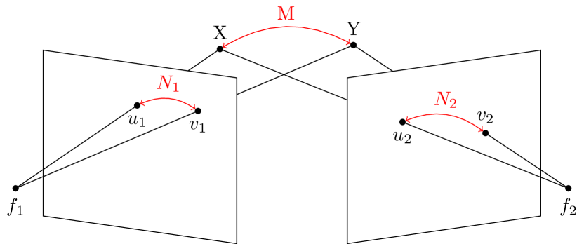
If m=2𝑚2m=2 we can use symmetric matrices in Sym2(4)subscriptSym2superscript4\operatorname*{Sym}_{2}(\mathbb{R}^{4}) and Sym2(3)subscriptSym2superscript3\operatorname*{Sym}_{2}(\mathbb{R}^{3}) to describe the unlabeled multiview variety, even for n𝑛n larger than two. This is computationally easier to handle. Then the unlabeled world point configuration of the two labeled world points X,Y3𝑋𝑌superscript3X,Y\in\mathbb{P}^{3} can be represented by a symmetric 4×4444\times 4 rank two matrix M=XYT+YXT𝑀𝑋superscript𝑌𝑇𝑌superscript𝑋𝑇M=XY^{T}+YX^{T}. The unlabeled image point configuration of two labeled image points in the i𝑖i-th picture ui,vi2subscript𝑢𝑖subscript𝑣𝑖superscript2u_{i},v_{i}\in\mathbb{P}^{2} can be represented by the symmetric 3×3333\times 3 rank two matrix Ni=uiviT+viuiTsubscript𝑁𝑖subscript𝑢𝑖superscriptsubscript𝑣𝑖𝑇subscript𝑣𝑖superscriptsubscript𝑢𝑖𝑇N_{i}=u_{i}v_{i}^{T}+v_{i}u_{i}^{T}.

Remark 1.3.

Since X,Y,ui,vi𝑋𝑌subscript𝑢𝑖subscript𝑣𝑖X,\,Y,\,u_{i},\,v_{i} are points in projective spaces the symmetric rank two matrices M,Ni𝑀subscript𝑁𝑖M,\,N_{i} are only defined up to scale.

Refer to caption
Figure 1. Unlabeled two-view geometry

For a symmetric 4×4444\times 4 rank two matrix M𝑀M that is suitably generic, ξAsubscript𝜉𝐴\xi_{A} maps the matrix M𝑀M to n𝑛n symmetric 3×3333\times 3 of rank two matrices. Thus the unlabeled analog of the perspective relation AX=λu𝐴𝑋𝜆𝑢AX=\lambda u for a pinhole camera A3×4𝐴superscript34A\in\mathbb{R}^{3\times 4} reads as

(3) A(XYT+YXT=M)AT=λ(uvT+vuT=N),λ{0}formulae-sequence𝐴subscript𝑋superscript𝑌𝑇𝑌superscript𝑋𝑇absent𝑀superscript𝐴𝑇𝜆subscript𝑢superscript𝑣𝑇𝑣superscript𝑢𝑇absent𝑁𝜆0A(\underbrace{XY^{T}+YX^{T}}_{=M})A^{T}=\lambda(\underbrace{uv^{T}+vu^{T}}_{=N}),\,\lambda\in\mathbb{R}\setminus\{0\}

The unlabeled multiview map of two points is

(4) ξA:Sym2(3)Sym2(4)(Sym2(4))n,M(A1MA1T,,AnMAnT).:subscript𝜉𝐴absentsubscriptSym2superscript3subscriptSym2superscript4superscriptsubscriptSym2superscript4𝑛missing-subexpressionmissing-subexpressionmissing-subexpression𝑀maps-tosubscript𝐴1𝑀superscriptsubscript𝐴1𝑇subscript𝐴𝑛𝑀superscriptsubscript𝐴𝑛𝑇\begin{array}[]{llllll}\xi_{A}:&\operatorname*{Sym}_{2}(\mathbb{P}^{3})&\hookrightarrow&\operatorname*{Sym}_{2}(\mathbb{R}^{4})&\dashrightarrow&\bigl{(}\operatorname*{Sym}_{2}(\mathbb{R}^{4})\bigr{)}^{n},\\ &&&M&\mapsto&(A_{1}MA_{1}^{T},\ldots,A_{n}MA_{n}^{T}).\end{array}

If m=2𝑚2m=2 the unlabeled multiview variety Sym2(VA)subscriptSym2subscript𝑉𝐴\operatorname*{Sym}_{2}(V_{A}) is the closure of the image of the rational map ξAsubscript𝜉𝐴\xi_{A}.

We will pay special attention to the algebraic variety V(ξA)𝑉subscript𝜉𝐴V(\xi_{A}) of the closure of the image of ξAsubscript𝜉𝐴\xi_{A} in Section 3.

2. Relabeling the Unlabeled

The Chow variety is a tool to easier handle unlabeled points, in order to understand the geometry it is sometimes more convenient not to think about unlabeled points as symmetric tensors. While in the section above we viewed two unlabeled points as one point on the Chow variety Symm(2)subscriptSym𝑚superscript2\operatorname*{Sym}_{m}(\mathbb{P}^{2}), in this section we will stick to unlabeled points as points in 2superscript2\mathbb{P}^{2} and 3superscript3\mathbb{P}^{3}. Let ρ𝜌\rho be the map that takes a labeled point configuration in (2)msuperscriptsuperscript2𝑚(\mathbb{P}^{2})^{m} to its unlabeled configuration represented as a symmetric tensor, e.g. if n=2𝑛2n=2, m=2𝑚2m=2 then ρ𝜌\rho takes (u,v)𝑢𝑣(u,v) and (v,u)𝑣𝑢(v,u), both in 2×2superscript2superscript2\mathbb{P}^{2}\times\mathbb{P}^{2}, to the same symmetric matrix uvT+vuT𝑢superscript𝑣𝑇𝑣superscript𝑢𝑇uv^{T}+vu^{T}. The preimage of the unlabeled multiview variety under the map ρ𝜌\rho is the union of labeled multiview varieties with the labeling of their image points interchanged.
Refer to caption
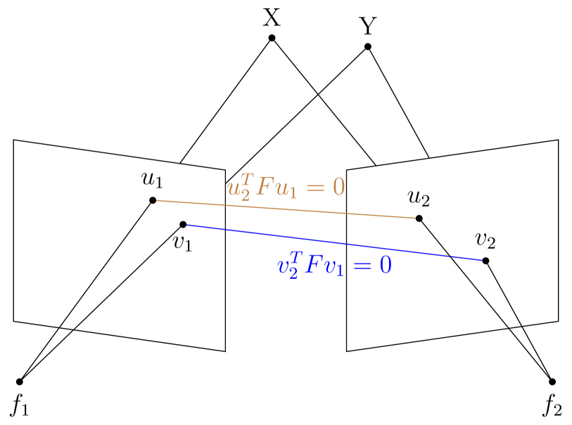
(a) u1u2,v1v2formulae-sequencesubscript𝑢1subscript𝑢2subscript𝑣1subscript𝑣2u_{1}\thicksim u_{2},\,v_{1}\thicksim v_{2}
Refer to caption
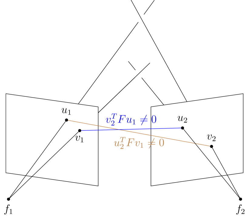
(b) v1u2,u1v2formulae-sequencesubscript𝑣1subscript𝑢2subscript𝑢1subscript𝑣2v_{1}\thicksim u_{2},\,u_{1}\thicksim v_{2}
Figure 2. The two multiview varieties with permuted image point correspondence
Example 2.1.

The image points u1,v1,u2,v22subscript𝑢1subscript𝑣1subscript𝑢2subscript𝑣2superscript2u_{1},v_{1},u_{2},v_{2}\in\mathbb{P}^{2} are on the product of two two-view varieties if they satisfy

u2TFu1=0 and v2TFv1=0.superscriptsubscript𝑢2𝑇𝐹subscript𝑢10 and superscriptsubscript𝑣2𝑇𝐹subscript𝑣10u_{2}^{T}Fu_{1}=0\text{ and }v_{2}^{T}Fv_{1}=0.

The image points u1,v1,u2,v22subscript𝑢1subscript𝑣1subscript𝑢2subscript𝑣2superscript2u_{1},v_{1},u_{2},v_{2}\in\mathbb{P}^{2} are on the the closure of the preimage under ρ𝜌\rho of the unlabeled two-view variety of two points if they satisfy (s. Figure 2)

(5) (u2TFu1=0 and v2TFv1=0) or (v2TFu1=0 and u2TFv1=0).\bigr{(}u_{2}^{T}Fu_{1}=0\text{ and }v_{2}^{T}Fv_{1}=0\bigr{)}\text{ or }\bigl{(}v_{2}^{T}Fu_{1}=0\text{ and }u_{2}^{T}Fv_{1}=0\bigr{)}.

This variety is cut out set-theoretically by the ideal

(u2TFu1)(v2TFu1),(u2TFu1)(u2TFv1),(v2TFv1)(v2TFu1),(v2TFv1)(u2TFv1).superscriptsubscript𝑢2𝑇𝐹subscript𝑢1superscriptsubscript𝑣2𝑇𝐹subscript𝑢1superscriptsubscript𝑢2𝑇𝐹subscript𝑢1superscriptsubscript𝑢2𝑇𝐹subscript𝑣1superscriptsubscript𝑣2𝑇𝐹subscript𝑣1superscriptsubscript𝑣2𝑇𝐹subscript𝑢1superscriptsubscript𝑣2𝑇𝐹subscript𝑣1superscriptsubscript𝑢2𝑇𝐹subscript𝑣1\bigl{\langle}(u_{2}^{T}Fu_{1})(v_{2}^{T}Fu_{1}),(u_{2}^{T}Fu_{1})(u_{2}^{T}Fv_{1}),(v_{2}^{T}Fv_{1})(v_{2}^{T}Fu_{1}),(v_{2}^{T}Fv_{1})(u_{2}^{T}Fv_{1})\bigr{\rangle}.

The approach of Example 2.1 extends to more pictures and more unlabeled world points. The idea here is to permute the labeling of the image points in each picture. Each permutation of image points gives a new product of multiview varieties with permuted coordinates. The union over all these product varieties then is the unlabeled multiview variety.

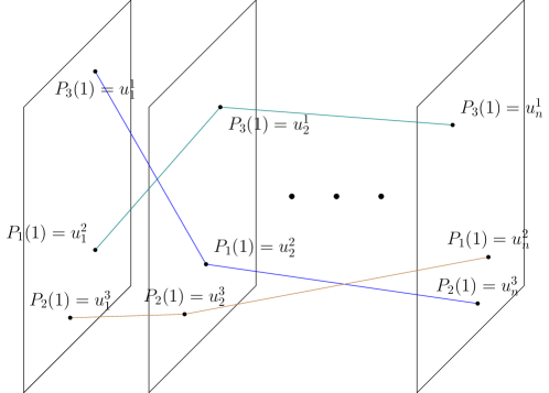
We construct a graph with all the image points as vertices, see Figure 3. Let G𝐺G be the n𝑛n-partite complete graph on nm𝑛𝑚n\cdot m vertices, where each partition of G𝐺G has cardinality m𝑚m. Let KG𝐾𝐺K\subset G be a perfect n𝑛n-dimensional matching and by 𝒦𝒦\mathcal{K} we denote the set of all such perfect n𝑛n-dimensional matchings on G𝐺G. For a fixed K𝐾K we denote Pi(j)subscript𝑃𝑖𝑗P_{i}(j), that is an image point ujsuperscriptsubscript𝑢𝑗u_{j}^{*} in the j𝑗j-th picture, as the vertex in the j𝑗j-th partition of G𝐺G in the i𝑖i-th path Pisubscript𝑃𝑖P_{i} of K𝐾K, with i[n],j[m]formulae-sequence𝑖delimited-[]𝑛𝑗delimited-[]𝑚i\in[n],\,j\in[m].

In this section we have not been working with unlabeled points in Symm(2)subscriptSym𝑚superscript2\operatorname*{Sym}_{m}(\mathbb{P}^{2}) but with labeled points (2)msuperscriptsuperscript2𝑚(\mathbb{P}^{2})^{m} and their orbits under group action on the image points of the symmetric group. The following theorem illustrates the relation between these two approaches.

Proposition 2.2.

The closure of the preimage under ρ𝜌\rho of the unlabeled multiview variety is the union of products of multiview varieties, with permuted image points correspondences

K𝒦(VA(P1(1),P2(1),,Pn(1))××VA(P1(m),P2(m),,Pn(m))).subscript𝐾𝒦subscript𝑉𝐴subscript𝑃11subscript𝑃21subscript𝑃𝑛1subscript𝑉𝐴subscript𝑃1𝑚subscript𝑃2𝑚subscript𝑃𝑛𝑚\bigcup_{K\in\mathcal{K}}\Bigl{(}V_{A}\bigl{(}{P_{1}(1)},{P_{2}(1)},\ldots,{P_{n}(1)}\bigr{)}\times\ldots\times V_{A}\bigl{(}{P_{1}(m)},{P_{2}(m)},\ldots,{P_{n}(m)}\bigr{)}\Bigr{)}.
Proof.

The usual multiview variety knows the labeling of the images points, however the unlabeled does not. Thus the unlabeled variety is nothing but the union of all multiview varieties with permuted image point correspondences. A permuted image point correspondence is an n𝑛n-dimensional matching through the n𝑛n images, as depicted in Figure 3. Taking the union over all such possible correspondences yields the preimage of the the unlabeled multiview variety. ∎
Refer to caption
Figure 3. Permuted image point correspondence graph
Remark 2.3.

The multiview variety is cut out set-theoretically by the bilinear constraints, if the cameras are in linearly general position [5]. Thus the unlabeled multiview variety is cut out by the products of bilinear constraints.

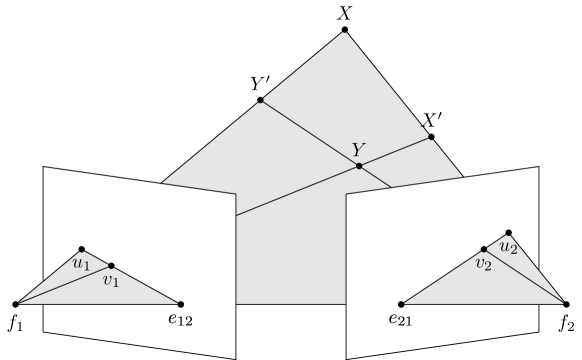
The usual two-view triangulation does result in either zero solutions (u1subscript𝑢1u_{1}, u2subscript𝑢2u_{2} are not on the two-view variety), one solutions (u1subscript𝑢1u_{1}, u2subscript𝑢2u_{2} are on the two-view variety) or a one dimensional linear subspace of solutions (u1subscript𝑢1u_{1}, u2subscript𝑢2u_{2} are the epipoles). The situation is a little different if we forget the labeling of the image points. Anyway, the triangulation problem still amounts in intersecting the back-projected lines. The reconstruction of the original world points is called unlabeled triangulation. In the following its ambiguities are studied. The unlabeled triangulation is ambiguous if there are two or more unlabeled world point configurations that project down to the same unlabeled image point configuration.
Refer to caption
Figure 4. Ambiguous unlabeled two-view triangulation
Proposition 2.4.

Let n=m=2. The unlabeled triangulation is not unique, if and only if the image points are on the unlabeled multiview variety and satisfy the two conditions

|e12,u1,v1|=0,|e21,u2,v2|=0.\begin{array}[]{cc}|e_{12},u_{1},v_{1}|=0,&|e_{21},u_{2},v_{2}|=0\end{array}.

If the image points u1,u2,v1,v2subscript𝑢1subscript𝑢2subscript𝑣1subscript𝑣2u_{1},u_{2},v_{1},v_{2} are distinct from the epipoles e1,e2subscript𝑒1subscript𝑒2e_{1},e_{2}, then there are exactly two possible unlabeled world point pairs (X,Y)𝑋𝑌(X,Y) and (X,Y)superscript𝑋superscript𝑌(X^{\prime},Y^{\prime}) that are possible reconstructions.

Proof.

By construction the arrangement of the four back-projected lines of u1,u2,v1,v2subscript𝑢1subscript𝑢2subscript𝑣1subscript𝑣2u_{1},u_{2},v_{1},v_{2} have the focal points f1subscript𝑓1f_{1} and f2subscript𝑓2f_{2} as intersection points. Such that the triangulation is ambiguous the four back-projected lines must have at least four additional intersections. Thus the back-projected lines need to be coplanar by the Veblen-Young axiom. Because u1,u2,v1,v2subscript𝑢1subscript𝑢2subscript𝑣1subscript𝑣2u_{1},u_{2},v_{1},v_{2} are on the unlabeled multiview variety this is equivalent to eij,u1,v1subscript𝑒𝑖𝑗subscript𝑢1subscript𝑣1e_{ij},u_{1},v_{1} being collinear, as depicted in Figure 4. Now if e12,u1,v1subscript𝑒12subscript𝑢1subscript𝑣1e_{12},u_{1},v_{1} are pairwise distinct and e21,u2,v2subscript𝑒21subscript𝑢2subscript𝑣2e_{21},u_{2},v_{2} are pairwise distinct, then the back-projected lines have in total six intersections of which four are not the focal points. ∎

Remark 2.5.

Let n=m=2. In world coordinates the ambiguity of the unlabeled triangulation revolves around the world points X𝑋X, Y𝑌Y and the baseline β12subscript𝛽12\beta_{12} through the focal points f1,f2subscript𝑓1subscript𝑓2f_{1},f_{2} being coplanar. Hence the pencil of planes with the baseline β12subscript𝛽12\beta_{12} as its axis encodes the ambiguities of the two view unlabeled triangulation.

The ambiguity of the unlabeled triangulation of two views and two unlabeled points extends to the case n=2,m2formulae-sequence𝑛2𝑚2n=2,m\geq 2.

Corollary 2.6.

If a subset of the world point configuration and the baseline βijsubscript𝛽𝑖𝑗\beta_{ij} are coplanar, then the unlabeled triangulation is ambiguous.

Proof.

Follows immediately from Proposition 2.4. ∎

When a subset of k𝑘k unlabeled world points and the baseline are on one plane, then all their back-projected lines intersect each other pairwise. There are in total k2superscript𝑘2k^{2} such intersection points. To construct an alternative world point configurations, each back-projected line has to be used exactly one time. Otherwise the resulting image point configuration does not align with the original image point configuration.

Remark 2.7.

Consider k𝑘k world points that are coplanar with the baseline, then there are k!𝑘k! different solutions to the unlabeled triangulation from two views.

For generic points on the unlabeled multiview variety the back-projected lines intersect in only two points and the reconstructing of the unlabeled world point configuration is unique.

When m>2𝑚2m>2 the back-projected lines represent a line arrangement in 3superscript3\mathbb{P}^{3}, where through each focal point m𝑚m lines pass. Let the intersection degree of a point in 3superscript3\mathbb{P}^{3} denote the number of back-projected lines that intersect in that point. The unlabeled triangulation amounts in finding points in 3superscript3\mathbb{P}^{3} with intersection degree equal to n𝑛n that are distinct from the focal points. A configuration of world points is a valid triangulation of the image points if it covers all back-projected lines.

Refer to caption
Figure 5. The blue and brown vertices describe different world point configurations that project to the same unlabeled image point configuration. The dashed lines denote the missing incidences in Pappus’s hexagon theorem.

In general classifying the ambiguities of the unlabeled triangulation is a complex problem.

For three views n=3𝑛3n=3 and three unlabeled points one can employ Pappus’s hexagon theorem to construct an ambiguous unlabeled triangulation. In this case a configuration that possesses an ambiguous unlabeled triangulation must lie on the trifocal plane. Figure 5 depicts such an situation on the trifocal plane.

3. Two Unlabeled Points

In this section we will only consider the case of two (m=2) unlabeled world points. The complicated part of the unlabeled multiview map of Equation 4 is the rank two constraint on the symmetric matrix M𝑀M. However if M𝑀M has rank two we can be sure that its projections Nisubscript𝑁𝑖N_{i} have rank two.

Lemma 3.1.

The matrices Nisubscript𝑁𝑖N_{i} have rank at most two if M𝑀M has rank two. If M=XYT+YXT𝑀𝑋superscript𝑌𝑇𝑌superscript𝑋𝑇M=XY^{T}+YX^{T}, then N𝑁N can be written as Ni=uvT+vuTsubscript𝑁𝑖𝑢superscript𝑣𝑇𝑣superscript𝑢𝑇N_{i}=uv^{T}+vu^{T} for some u,v2𝑢𝑣superscript2u,v\in\mathbb{P}^{2}.

Proof.

If M𝑀M has rank two, then rk(Ni)=rk(AiMAiT)2rksubscript𝑁𝑖rksubscript𝐴𝑖𝑀superscriptsubscript𝐴𝑖𝑇2\operatorname*{rk}(N_{i})=\operatorname*{rk}(A_{i}MA_{i}^{T})\leq 2. The second statement is obtained from the fact

Ai(XYT+YXT)AiT=AiX(YAi)T+AiY(XAi)T=λiuvT+vuT=λNi.subscript𝐴𝑖𝑋superscript𝑌𝑇𝑌superscript𝑋𝑇superscriptsubscript𝐴𝑖𝑇subscript𝐴𝑖𝑋superscript𝑌subscript𝐴𝑖𝑇subscript𝐴𝑖𝑌superscript𝑋subscript𝐴𝑖𝑇subscript𝜆𝑖𝑢superscript𝑣𝑇𝑣superscript𝑢𝑇𝜆subscript𝑁𝑖A_{i}(XY^{T}+YX^{T})A_{i}^{T}=A_{i}X(YA_{i})^{T}+A_{i}Y(XA_{i})^{T}=\lambda_{i}uv^{T}+vu^{T}=\lambda N_{i}.

Remark 3.2.

The reverse of the second statement of Lemma 3.1 does not hold Ni=uvT+vuTiM=XYT+YXTsubscript𝑁𝑖𝑢superscript𝑣𝑇𝑣superscript𝑢𝑇for-all𝑖𝑀𝑋superscript𝑌𝑇𝑌superscript𝑋𝑇N_{i}=uv^{T}+vu^{T}\,\forall\,i\nRightarrow M=XY^{T}+YX^{T}

We first analyze Sym2(VA)subscriptSym2subscript𝑉𝐴\operatorname*{Sym}_{2}(V_{A}) by dropping the rank two constraints in ξAsubscript𝜉𝐴\xi_{A}. This gives us the rational map

θA:Sym2(4)(Sym2(3))n,M(A1MA1T,,AnMAnT).:subscript𝜃𝐴absentsubscriptSym2superscript4superscriptsubscriptSym2superscript3𝑛missing-subexpression𝑀maps-tosubscript𝐴1𝑀superscriptsubscript𝐴1𝑇subscript𝐴𝑛𝑀superscriptsubscript𝐴𝑛𝑇\begin{array}[]{llll}\theta_{A}:&\operatorname*{Sym}_{2}(\mathbb{R}^{4})&\dashrightarrow&\bigl{(}\operatorname*{Sym}_{2}(\mathbb{R}^{3})\bigr{)}^{n},\\ &M&\mapsto&(A_{1}MA_{1}^{T},\ldots,A_{n}MA_{n}^{T}).\end{array}

We will denote the ideal and the variety of the closure of the image of as Iθsubscript𝐼𝜃I_{\theta} and Vθsubscript𝑉𝜃V_{\theta}. This variety is a relaxation of the unlabeled multiview variety Sym2(VA)subscriptSym2subscript𝑉𝐴\operatorname*{Sym}_{2}(V_{A}). The map θAsubscript𝜃𝐴\theta_{A} is linear in the entries of the symmetric matrix M𝑀M, thus by row-wise vectorizing the upper triangular entries of MSym2(4)𝑀subscriptSym2superscript4M\in\operatorname*{Sym}_{2}(\mathbb{R}^{4}) to \vvM10\vv𝑀superscript10\vv{M}\in\mathbb{R}^{10} the map θAsubscript𝜃𝐴\theta_{A} can be rewritten in its standard form of linear equations, with the coefficient matrices A~isubscript~𝐴𝑖\widetilde{A}_{i}. In the coordinates of Ai=(ajk)j[3],k[4]subscript𝐴𝑖subscriptsubscript𝑎𝑗𝑘formulae-sequence𝑗delimited-[]3𝑘delimited-[]4A_{i}=(a_{jk})_{j\in[3],k\in[4]} the coefficient matrix A~isubscript~𝐴𝑖\widetilde{A}_{i} then reads as

A~i=(a112a11a21a11a31a212a21a31a3122a11a12a12a21+a11a22a12a31+a11a322a21a22a22a31+a21a322a31a322a11a13a13a21+a11a23a13a31+a11a332a21a23a23a31+a21a332a31a332a11a14a14a21+a11a24a14a31+a11a342a21a24a24a31+a21a342a31a34a122a12a22a12a32a222a22a32a3222a12a13a13a22+a12a23a13a32+a12a332a22a23a23a32+a22a332a32a332a12a14a14a22+a12a24a14a32+a12a342a22a24a24a32+a22a342a32a34a132a13a23a13a33a232a23a33a3322a13a14a14a23+a13a24a14a33+a13a342a23a24a24a33+a23a342a33a34a142a14a24a14a34a242a24a34a342)subscript~𝐴𝑖matrixsuperscriptsubscript𝑎112subscript𝑎11subscript𝑎21subscript𝑎11subscript𝑎31superscriptsubscript𝑎212subscript𝑎21subscript𝑎31superscriptsubscript𝑎3122subscript𝑎11subscript𝑎12subscript𝑎12subscript𝑎21subscript𝑎11subscript𝑎22subscript𝑎12subscript𝑎31subscript𝑎11subscript𝑎322subscript𝑎21subscript𝑎22subscript𝑎22subscript𝑎31subscript𝑎21subscript𝑎322subscript𝑎31subscript𝑎322subscript𝑎11subscript𝑎13subscript𝑎13subscript𝑎21subscript𝑎11subscript𝑎23subscript𝑎13subscript𝑎31subscript𝑎11subscript𝑎332subscript𝑎21subscript𝑎23subscript𝑎23subscript𝑎31subscript𝑎21subscript𝑎332subscript𝑎31subscript𝑎332subscript𝑎11subscript𝑎14subscript𝑎14subscript𝑎21subscript𝑎11subscript𝑎24subscript𝑎14subscript𝑎31subscript𝑎11subscript𝑎342subscript𝑎21subscript𝑎24subscript𝑎24subscript𝑎31subscript𝑎21subscript𝑎342subscript𝑎31subscript𝑎34superscriptsubscript𝑎122subscript𝑎12subscript𝑎22subscript𝑎12subscript𝑎32superscriptsubscript𝑎222subscript𝑎22subscript𝑎32superscriptsubscript𝑎3222subscript𝑎12subscript𝑎13subscript𝑎13subscript𝑎22subscript𝑎12subscript𝑎23subscript𝑎13subscript𝑎32subscript𝑎12subscript𝑎332subscript𝑎22subscript𝑎23subscript𝑎23subscript𝑎32subscript𝑎22subscript𝑎332subscript𝑎32subscript𝑎332subscript𝑎12subscript𝑎14subscript𝑎14subscript𝑎22subscript𝑎12subscript𝑎24subscript𝑎14subscript𝑎32subscript𝑎12subscript𝑎342subscript𝑎22subscript𝑎24subscript𝑎24subscript𝑎32subscript𝑎22subscript𝑎342subscript𝑎32subscript𝑎34superscriptsubscript𝑎132subscript𝑎13subscript𝑎23subscript𝑎13subscript𝑎33superscriptsubscript𝑎232subscript𝑎23subscript𝑎33superscriptsubscript𝑎3322subscript𝑎13subscript𝑎14subscript𝑎14subscript𝑎23subscript𝑎13subscript𝑎24subscript𝑎14subscript𝑎33subscript𝑎13subscript𝑎342subscript𝑎23subscript𝑎24subscript𝑎24subscript𝑎33subscript𝑎23subscript𝑎342subscript𝑎33subscript𝑎34superscriptsubscript𝑎142subscript𝑎14subscript𝑎24subscript𝑎14subscript𝑎34superscriptsubscript𝑎242subscript𝑎24subscript𝑎34superscriptsubscript𝑎342\widetilde{A}_{i}=\footnotesize\begin{pmatrix}{a}_{11}^{2}&{a}_{11}{a}_{21}&{a}_{11}{a}_{31}&{a}_{21}^{2}&{a}_{21}{a}_{31}&{a}_{31}^{2}\\ 2{a}_{11}{a}_{12}&{a}_{12}{a}_{21}+{a}_{11}{a}_{22}&{a}_{12}{a}_{31}+{a}_{11}{a}_{32}&2{a}_{21}{a}_{22}&{a}_{22}{a}_{31}+{a}_{21}{a}_{32}&2{a}_{31}{a}_{32}\\ 2{a}_{11}{a}_{13}&{a}_{13}{a}_{21}+{a}_{11}{a}_{23}&{a}_{13}{a}_{31}+{a}_{11}{a}_{33}&2{a}_{21}{a}_{23}&{a}_{23}{a}_{31}+{a}_{21}{a}_{33}&2{a}_{31}{a}_{33}\\ 2{a}_{11}{a}_{14}&{a}_{14}{a}_{21}+{a}_{11}{a}_{24}&{a}_{14}{a}_{31}+{a}_{11}{a}_{34}&2{a}_{21}{a}_{24}&{a}_{24}{a}_{31}+{a}_{21}{a}_{34}&2{a}_{31}{a}_{34}\\ {a}_{12}^{2}&{a}_{12}{a}_{22}&{a}_{12}{a}_{32}&{a}_{22}^{2}&{a}_{22}{a}_{32}&{a}_{32}^{2}\\ 2{a}_{12}{a}_{13}&{a}_{13}{a}_{22}+{a}_{12}{a}_{23}&{a}_{13}{a}_{32}+{a}_{12}{a}_{33}&2{a}_{22}{a}_{23}&{a}_{23}{a}_{32}+{a}_{22}{a}_{33}&2{a}_{32}{a}_{33}\\ 2{a}_{12}{a}_{14}&{a}_{14}{a}_{22}+{a}_{12}{a}_{24}&{a}_{14}{a}_{32}+{a}_{12}{a}_{34}&2{a}_{22}{a}_{24}&{a}_{24}{a}_{32}+{a}_{22}{a}_{34}&2{a}_{32}{a}_{34}\\ {a}_{13}^{2}&{a}_{13}{a}_{23}&{a}_{13}{a}_{33}&{a}_{23}^{2}&{a}_{23}{a}_{33}&{a}_{33}^{2}\\ 2{a}_{13}{a}_{14}&{a}_{14}{a}_{23}+{a}_{13}{a}_{24}&{a}_{14}{a}_{33}+{a}_{13}{a}_{34}&2{a}_{23}{a}_{24}&{a}_{24}{a}_{33}+{a}_{23}{a}_{34}&2{a}_{33}{a}_{34}\\ {a}_{14}^{2}&{a}_{14}{a}_{24}&{a}_{14}{a}_{34}&{a}_{24}^{2}&{a}_{24}{a}_{34}&{a}_{34}^{2}\\ \end{pmatrix}

and the according rational map is

(6) θ~A:9(5)n,\vvM(A~1\vvM,,A~n\vvM),:subscript~𝜃𝐴absentsuperscript9superscriptsuperscript5𝑛missing-subexpression\vv𝑀maps-tosubscript~𝐴1\vv𝑀subscript~𝐴𝑛\vv𝑀\begin{array}[]{llll}\widetilde{\theta}_{A}:&\mathbb{P}^{9}&\dashrightarrow&(\mathbb{P}^{5})^{n},\\ &\vv{M}&\mapsto&(\widetilde{A}_{1}\vv M,\ldots,\widetilde{A}_{n}\vv M),\end{array}

This map strongly resembles the conventional multiview map of Equation 2 and can be understood as a higher dimensional analogue of it. We use the techniques developed in [7] for a more general setup to describe the closure of the image of θ~Asubscript~𝜃𝐴\widetilde{\theta}_{A} in Corollary 3.7. But we first study the unlabeled triangulation. The results we obtain to understand the unlabeled triangulation will come in handy for Corollary 3.7.

Let σ[n]𝜎delimited-[]𝑛\sigma\subseteq[n] with |σ|=k𝜎𝑘|\sigma|=k and A~σ=(A~σ1T,,A~σkT)subscript~𝐴𝜎superscriptsubscript~𝐴subscript𝜎1𝑇superscriptsubscript~𝐴subscript𝜎𝑘𝑇\widetilde{A}_{\sigma}=(\widetilde{A}_{\sigma_{1}}^{T},\ldots,\widetilde{A}_{\sigma_{k}}^{T}), then define Bσsubscript𝐵𝜎B_{\sigma} as

(7) Bσ=[A~σ1\vvNσ1A~σk\vvNσk].subscript𝐵𝜎matrixsubscript~𝐴subscript𝜎1\vvsubscript𝑁subscript𝜎1missing-subexpressionmissing-subexpressionmissing-subexpressionmissing-subexpressionsubscript~𝐴subscript𝜎𝑘missing-subexpressionmissing-subexpression\vvsubscript𝑁subscript𝜎𝑘B_{\sigma}=\begin{bmatrix}\widetilde{A}_{\sigma_{1}}&\vv N_{\sigma_{1}}&&\\ \vdots&&\ddots&\\ \widetilde{A}_{\sigma_{k}}&&&\vv N_{\sigma_{k}}\end{bmatrix}.

Let the unlabeled focal point fijsubscript𝑓𝑖𝑗f_{ij} of the cameras Aisubscript𝐴𝑖A_{i} and Ajsubscript𝐴𝑗A_{j} be fij:=fifjT+fjfiTassignsubscript𝑓𝑖𝑗subscript𝑓𝑖superscriptsubscript𝑓𝑗𝑇subscript𝑓𝑗superscriptsubscript𝑓𝑖𝑇f_{ij}:=f_{i}f_{j}^{T}+f_{j}f_{i}^{T}.

Proposition 3.3.

Let n=m=2𝑛𝑚2n=m=2. Let N1subscript𝑁1N_{1} and N2subscript𝑁2N_{2} be two generic points on the unlabeled two-view variety and denote their unlabeled triangulation MΔ=XYT+YXTsubscript𝑀Δ𝑋superscript𝑌𝑇𝑌superscript𝑋𝑇M_{\Delta}=XY^{T}+YX^{T}. Then rk(B{1,2})=10rksubscript𝐵1210\operatorname*{rk}(B_{\{1,2\}})=10 and there exists λ1,λ2subscript𝜆1subscript𝜆2\lambda_{1},\,\lambda_{2}\in\mathbb{R}, such that

span((\vvf12,0,0)T,(\vvMΔ,λ1,λ2)T)=ker(B{1,2}).spansuperscript\vvsubscript𝑓1200𝑇superscript\vvsubscript𝑀Δsubscript𝜆1subscript𝜆2𝑇kernelsubscript𝐵12\operatorname*{span}\bigl{(}(\vv{f_{12}},0,0)^{T},(\vv M_{\Delta},\lambda_{1},\lambda_{2})^{T}\bigr{)}=\ker(B_{\{1,2\}}).
Proof.

Since N1subscript𝑁1N_{1} and N2subscript𝑁2N_{2} are generic points on the unlabeled multiview variety the triangulation is unique and MΔ=XYT+YXTsubscript𝑀Δ𝑋superscript𝑌𝑇𝑌superscript𝑋𝑇M_{\Delta}=XY^{T}+YX^{T} is its solution. Hence there are λ1,λ2subscript𝜆1subscript𝜆2\lambda_{1},\,\lambda_{2}, such that (\vvMΔ,λ1,λ2)\vvsubscript𝑀Δsubscript𝜆1subscript𝜆2(\vv M_{\Delta},\lambda_{1},\lambda_{2}) is in ker(B{1,2})kernelsubscript𝐵12\ker(B_{\{1,2\}}). On the other hand A~i\vvM=λi\vvNisubscript~𝐴𝑖\vv𝑀subscript𝜆𝑖\vvsubscript𝑁𝑖\widetilde{A}_{i}\vv M=\lambda_{i}\vv N_{i} is equivalent to AiMAiT=λiNisubscript𝐴𝑖𝑀superscriptsubscript𝐴𝑖𝑇subscript𝜆𝑖subscript𝑁𝑖A_{i}MA_{i}^{T}=\lambda_{i}N_{i}, thus inserting f1f2T+f2f1Tsubscript𝑓1superscriptsubscript𝑓2𝑇subscript𝑓2superscriptsubscript𝑓1𝑇f_{1}f_{2}^{T}+f_{2}f_{1}^{T} gives A1(f1f2T+f2f1T)A1T=0subscript𝐴1subscript𝑓1superscriptsubscript𝑓2𝑇subscript𝑓2superscriptsubscript𝑓1𝑇superscriptsubscript𝐴1𝑇0A_{1}\left(f_{1}f_{2}^{T}+f_{2}f_{1}^{T}\right)A_{1}^{T}=0 and inserting gives A2(f2f1T+f1f2T)A2T=0subscript𝐴2subscript𝑓2superscriptsubscript𝑓1𝑇subscript𝑓1superscriptsubscript𝑓2𝑇superscriptsubscript𝐴2𝑇0A_{2}\left(f_{2}f_{1}^{T}+f_{1}f_{2}^{T}\right)A_{2}^{T}=0. Hence for λ1=λ2=0subscript𝜆1subscript𝜆20\lambda_{1}=\lambda_{2}=0 the vector (\vvf12,0,0)\vvsubscript𝑓1200(\vv f_{12},0,0) is in ker(B{1,2})kernelsubscript𝐵12\ker(B_{\{1,2\}}). ∎

Remark 3.4.

By the proof of Proposition 3.3 ker(A~{i,j})kernelsubscript~𝐴𝑖𝑗\ker(\widetilde{A}_{\{i,j\}}) is spanned by \vvfij\vvsubscript𝑓𝑖𝑗\vv f_{ij}.

Proposition 3.5.

Let n3𝑛3n\geq 3. For a generic choice of cameras A1,,Ansubscript𝐴1subscript𝐴𝑛A_{1},\ldots,A_{n} the matrix A~σsubscript~𝐴𝜎\widetilde{A}_{\sigma} has full rank.

Proof.

The unlabeled focal point fijsubscript𝑓𝑖𝑗f_{ij} is the kernel of the submatrix A~{i,j}subscript~𝐴𝑖𝑗\widetilde{A}_{\{i,j\}}. Since fijsubscript𝑓𝑖𝑗f_{ij} does not depend on the other cameras it is not in the kernel of any of the other A~ksubscript~𝐴𝑘\widetilde{A}_{k} for a generic choice of cameras. ∎

We can use the matrix Bσsubscript𝐵𝜎B_{\sigma} to design a triangulation algorithm for the unlabeled multiview variety. We call this algorithm the unlabeled triangulation algorithm. The Proposition 3.3 indicates that the unlabeled triangulation is more complicated than the usual labeled triangulation. By Propositions 2.4 and Corollary 2.6 it can have multiple solutions. Especially the case of two views is more elaborate. Nonetheless it has a unique solution for generic points on the unlabeled multiview variety. We need a lemma before we can state the unlabeled triangulation algorithm.

Lemma 3.6.

Consider a two-dimensional linear subspace VSym2(4)𝑉subscriptSym2superscript4V\subset\operatorname*{Sym}_{2}(\mathbb{R}^{4}) spanned by two symmetric matrices. Suppose that V𝑉V contains two distinct rank two symmetric matrices M1,M2Sym2(4)subscript𝑀1subscript𝑀2subscriptSym2superscript4M_{1},M_{2}\in\operatorname*{Sym}_{2}(\mathbb{R}^{4}), such that rk(M1M2)=4rksubscript𝑀1subscript𝑀24\operatorname*{rk}(M_{1}-M_{2})=4. Then the symmetric matrices M1,M2subscript𝑀1subscript𝑀2M_{1},M_{2} are the only rank two symmetric matrices in V𝑉V. Also the subspace V𝑉V contains no rank three symmetric matrix.

Proof.

We can choose M1subscript𝑀1M_{1} and M2subscript𝑀2M_{2} as basis of V𝑉V. The rank two matrices in V𝑉V can be computed as some roots of det(αM1+(1α)M2)𝛼subscript𝑀11𝛼subscript𝑀2\det(\alpha M_{1}+(1-\alpha)M_{2}). Clearly zero and one are roots of this univariate polynomial. However the roots of det(αM1+(1α)M2)𝛼subscript𝑀11𝛼subscript𝑀2\det(\alpha M_{1}+(1-\alpha)M_{2}) are the generalized eigenvalues to the matrix equation M1x=α(M2M1)x,x4formulae-sequencesubscript𝑀1𝑥𝛼subscript𝑀2subscript𝑀1𝑥𝑥superscript4M_{1}x=\alpha(M_{2}-M_{1})x,\,x\in\mathbb{R}^{4}. But since M1subscript𝑀1M_{1} has rank two the generalized eigenvalue α=0𝛼0\alpha=0 has double algebraic and geometric multiplicity. Then switching the roles of M1subscript𝑀1M_{1} and M2subscript𝑀2M_{2} shows that α=1𝛼1\alpha=1 also has double algebraic and geometric multiplicity. ∎

The unlabeled triangulation of two views results in finding the rank two matrices in linear two-dimensional subspaces. That subspace is constructed from ker(Bσ)kernelsubscript𝐵𝜎\ker(B_{\sigma}). We can find these matrices by finding the roots of a univariate quartic polynomial, as their determinant needs to vanish. If we only consider generic points on the unlabeled multiview variety, this polynomial has exactly two real solutions, the unlabeled focal point fijsubscript𝑓𝑖𝑗f_{ij} and the unlabeled triangulation MΔsubscript𝑀ΔM_{\Delta} of the unlabeled image points.

Input: N1,N2subscript𝑁1subscript𝑁2N_{1},N_{2} generic points on the unlabeled multiview variety;
Output: MΔsubscript𝑀ΔM_{\Delta} unlabeled triangulation of N1,N2subscript𝑁1subscript𝑁2N_{1},N_{2};
begin
      
  1. (1)

    Compute an element m𝑚m of kerBσkernelsubscript𝐵𝜎\ker{B_{\sigma}}, that is not a multiple of \vvf12\vvsubscript𝑓12\vv f_{12};

  2. (2)

    The first ten entries of m𝑚m represent a symmetric 4×4444\times 4 matrix M𝑀M;

  3. (3)

    Compute the quartic polynomial det(αM+(1α)f12)𝛼𝑀1𝛼subscript𝑓12\det(\alpha M+(1-\alpha)f_{12});

  4. (4)

    It factors to α2(αc)2,csuperscript𝛼2superscript𝛼𝑐2𝑐\alpha^{2}(\alpha-c)^{2},\,c\in\mathbb{R};

  5. (5)

    Compute c𝑐c; MΔ:=cM+(1c)f12assignsubscript𝑀Δ𝑐𝑀1𝑐subscript𝑓12M_{\Delta}:=cM+(1-c)f_{12};

end
Algorithm 1 Unlabeled triangulation problem for two views
Proof.

Since M𝑀M and f12subscript𝑓12f_{12} are symmetric with real entries det(αM+(1α)f12)𝛼𝑀1𝛼subscript𝑓12\det(\alpha M+(1-\alpha)f_{12}) only has real roots. By construction α=0𝛼0\alpha=0 is a root. Because (N1,N2)Sym2(VA)subscript𝑁1subscript𝑁2subscriptSym2subscript𝑉𝐴(N_{1},N_{2})\in\operatorname*{Sym}_{2}(V_{A}) there is a real value α=c𝛼𝑐\alpha=c such that MΔ:=cM+(1c)f12assignsubscript𝑀Δ𝑐𝑀1𝑐subscript𝑓12M_{\Delta}:=cM+(1-c)f_{12}. Now by Lemma 3.6 these two roots are the only roots of det(αM+(1α)f12)𝛼𝑀1𝛼subscript𝑓12\det(\alpha M+(1-\alpha)f_{12}). ∎

Since the roots of the univariate quartic polynomial det(αM+(1α)f12)𝛼𝑀1𝛼subscript𝑓12\det(\alpha M+(1-\alpha)f_{12}) have double multiplicity for generic points, we can find the roots by using the quadratic formula.

If n3𝑛3n\geq 3, then the procedure is simple and amounts to computing kerBσkernelsubscript𝐵𝜎\ker{B_{\sigma}}, because the kernel is one dimensional for generic data by Proposition 3.5. The complete triangulation algorithm can be stated as follows:

Input: N1,,Nnsubscript𝑁1subscript𝑁𝑛N_{1},\ldots,N_{n} generic points on the unlabeled multiview variety;
Output: MΔsubscript𝑀ΔM_{\Delta} unlabeled triangulation of N1,,Nnsubscript𝑁1subscript𝑁𝑛N_{1},\ldots,N_{n};
if n=2 then
       use Algorithm 1;
else
      
  1. (1)

    Compute the generator m𝑚m of kerBσkernelsubscript𝐵𝜎\ker{B_{\sigma}};

  2. (2)

    The first ten entries of m𝑚m represent the symmetric 4×4444\times 4 matrix MΔsubscript𝑀ΔM_{\Delta};

end if
Algorithm 2 Unlabeled triangulation problem
Proof.

The correctness of Algorithm 2 follows from the correctness of Algorithm 1. ∎

In some cases one might not want to keep on working with symmetric matrices, but actually reconstruct the original world points. This amounts to find a decomposition of MΔsuperscript𝑀ΔM^{\Delta} into XYT+YXT𝑋superscript𝑌𝑇𝑌superscript𝑋𝑇XY^{T}+YX^{T}. Finding such a decomposition is equivalent to splitting a degenerate quadrics 3superscript3\mathbb{P}^{3} into two planes. To do this, the approach studied in [8] for quadrics in 2superscript2\mathbb{P}^{2} generalizes to our case, if one replaces the adjoint matrix adj(MΔ)adjsuperscript𝑀Δ\operatorname*{adj}(M^{\Delta}) by the 6×6666\times 6 matrix of signed 2-minors of MΔsuperscript𝑀ΔM^{\Delta}.

We go back to studying the relaxed ideal Iθsubscript𝐼𝜃I_{{\theta}}. With the help of Proposition 3.3 we are able to determine the generators of the prime ideal Iθsubscript𝐼𝜃I_{{\theta}} of the image of θAsubscript𝜃𝐴\theta_{A}.

Corollary 3.7.

Let σ[n]𝜎delimited-[]𝑛\sigma\subseteq[n]. Then the ideal Iθsubscript𝐼𝜃I_{{\theta}} of the image of θAsubscript𝜃𝐴\theta_{A} is generated by the maximal minors of Bσsubscript𝐵𝜎B_{\sigma} (for all 3|σ|103𝜎103\leq|\sigma|\leq 10), and the 11-minors of Bσsubscript𝐵𝜎B_{\sigma} (for all |σ|=2𝜎2|\sigma|=2).

Proof.

By [7, §2.2] the ideal is generated by the rk(A~σ)+|σ|rksubscript~𝐴𝜎𝜎\operatorname*{rk}(\widetilde{A}_{\sigma})+|\sigma| minors of Bσsubscript𝐵𝜎B_{\sigma}. If |σ|=2𝜎2|\sigma|=2 then by the proof of Proposition 3.3 the matrix A~σsubscript~𝐴𝜎\widetilde{A}_{\sigma} has rank nine. If 3|σ|103𝜎103\leq|\sigma|\leq 10 then A~σsubscript~𝐴𝜎\widetilde{A}_{\sigma} has full rank by Proposition 3.5. Further maximal minors of matrices Bσsubscript𝐵𝜎B_{\sigma} with |σ|11𝜎11|\sigma|\geq 11 are monomial multiples of the other maximal minors. We obtain a generating set by just computing the minors of correct size. ∎

Remark 3.8.

Let n=2. Consider the ideal generated by the 11-minors and the ideal generated by the three degree (1,1)11(1,1) polynomials of Example 1.2. These two ideals are equal.

Clearly the relaxed ideal Iθsubscript𝐼𝜃I_{\theta} is not a good relaxation of Sym2(VA)subscriptSym2subscript𝑉𝐴\operatorname*{Sym}_{2}(V_{A}), but it can easily be tightened by enforcing the singularity condition det(Ni)=0subscript𝑁𝑖0\det(N_{i})=0. We define the ideal

Iθ:=Iθ+det(N1),,det(Nn).assignsubscriptsuperscript𝐼𝜃subscript𝐼𝜃𝑑𝑒𝑡subscript𝑁1𝑑𝑒𝑡subscript𝑁𝑛I^{\prime}_{\theta}:=I_{\theta}+\langle det(N_{1}),\ldots,det(N_{n})\rangle.

Still it is possible to construct rank two matrices on the variety V(Iθ)𝑉subscriptsuperscript𝐼𝜃V(I^{\prime}_{\theta}) that are not on Sym2(VA)subscriptSym2subscript𝑉𝐴\operatorname*{Sym}_{2}(V_{A}). Let be N1=e12vT+ve12T,v2formulae-sequencesubscript𝑁1subscript𝑒12superscript𝑣𝑇𝑣superscriptsubscript𝑒12𝑇𝑣superscript2N_{1}=e_{12}v^{T}+ve_{12}^{T},v\in\mathbb{P}^{2}. Then rk(B)10rk𝐵10\operatorname*{rk}(B)\leq 10 independent of N2subscript𝑁2N_{2}, thus requiring that the 11×11111111\times 11 minors of B𝐵B vanish (s. Corollary 3.7) does not impose any constraints on N2subscript𝑁2N_{2}. Remember that Equation 5 gives a description of the preimage of the unlabeled two-view variety of two points. However

(V(e12TFu2)×V(v1TFv2))(V(e12TFv2)×V(v1TFu2))𝑉superscriptsubscript𝑒12𝑇𝐹subscript𝑢2𝑉superscriptsubscript𝑣1𝑇𝐹subscript𝑣2𝑉superscriptsubscript𝑒12𝑇𝐹subscript𝑣2𝑉superscriptsubscript𝑣1𝑇𝐹subscript𝑢2\bigl{(}V(e_{12}^{T}Fu_{2})\times V(v_{1}^{T}Fv_{2})\bigr{)}\cup\bigl{(}V(e_{12}^{T}Fv_{2})\times V(v_{1}^{T}Fu_{2})\bigr{)}

gives constraints on v1,v2,u2subscript𝑣1subscript𝑣2subscript𝑢2v_{1},v_{2},u_{2}, namely (v2TFu1=0 or v2TFv1=0superscriptsubscript𝑣2𝑇𝐹subscript𝑢10 or superscriptsubscript𝑣2𝑇𝐹subscript𝑣10v_{2}^{T}Fu_{1}=0\text{ or }v_{2}^{T}Fv_{1}=0). Thus not all points of

(8) {(e12v1T+v1e12T,N2):v2,N2Sym3()}conditional-setsubscript𝑒12superscriptsubscript𝑣1𝑇subscript𝑣1superscriptsubscript𝑒12𝑇subscript𝑁2formulae-sequence𝑣superscript2subscript𝑁2subscriptSym3\bigl{\{}(e_{12}v_{1}^{T}+v_{1}e_{12}^{T},N_{2}):v\in\mathbb{P}^{2},N_{2}\in{\operatorname*{Sym}}_{3}(\mathbb{R})\bigr{\}}

are on the unlabeled multiview variety Sym2(VA)subscriptSym2subscript𝑉𝐴\operatorname*{Sym}_{2}(V_{A}), but they are on V(Iθ)𝑉subscriptsuperscript𝐼𝜃V(I^{\prime}_{\theta}).

Proposition 3.9.

For n=2, the unlabeled multiview variety is minimally generated by 7 polynomials in 12 variables. It is Cohen-Macaulay and its Betti table is given in Table 1.

Proof.

By Remark 4.4 of [1] the toric set-up of Remark 1.1 is universal in the sense that every multiview variety with cameras in linearly general position is isomorphic to the multiview variety of Remark 1.1. Since the unlabeled multiview variety with cameras in linearly general position is the union of multiview varieties with correspondences interchanges, any unlabeled multiview variety is isomorphic to the unlabeled multiview variety with the camera matrices of Remark 1.1. For two views we only chose the camera matrices A1subscript𝐴1A_{1} and A2subscript𝐴2A_{2} of Remark 1.1 and then ran the code of Listing 1 in Macaulay2[2] with these cameras as input. ∎

                                   0 1  2 3 4
                            total: 1 7 11 8 3
                                0: 1 .  . . .
                                1: . 3  2 . .
                                2: . 4  6 . .
                                3: . .  . 2 .
                                4: . .  3 6 3
Table 1. Betti numbers for the unlabeled multiview ideal with n=2𝑛2n=2.
Remark 3.10.

For cameras in linearly general position we have the freedom of choice of a world coordinate system in 3superscript3\mathbb{P}^{3} and coordinate systems in the images in 2superscript2\mathbb{P}^{2} without changing the unlabeled multiview variety up to isomorphism. In that sense we can freely choose five cameras with focal points in linearly general position to compute an isomorphic description of the unlabeled multiview variety.

As we see in Example 1.2 the generators of the unlabeled two-view variety of two points (n=2𝑛2n=2, m=2𝑚2m=2) fall into three different classes according to their multidegree, namely the ones with multidegree (1,1)11(1,1), the ones with degree type (2,1)21(2,1) and the ones with degree type (3,0)30(3,0). The ones of degree type (3,0)30(3,0) are the determinants of N1subscript𝑁1N_{1} and N2subscript𝑁2N_{2}.

Proposition 3.11.

The ideal of three degree (1,1)11(1,1) equations of the unlabeled two-view variety is a subset of the ideal generated by the entries of N2FN1subscript𝑁2𝐹subscript𝑁1N_{2}FN_{1}.

Proof.

The statement has been checked for sufficiently many random choices of camera pairs with Macaulay2[2], , see Section 5 for details. ∎

We currently have no way to construct the generators with degree type (2,1)21(2,1). However we do believe that they relate to the variety of Equation 8.

The following statements have been derived with Macaulay2[2]. They are concerned with the prime ideal of the unlabeled multiview variety of three, four and five views.

Proposition 3.12.

For n=3, the unlabeled multiview variety is minimally generated by 60 polynomials in 18 variables and its Betti table is given in Table 2.

Proof.

Similarly to the proof of Proposition 3.9 we choose special cameras to compute the unlabeled multiview variety. Here the cameras A1,A2subscript𝐴1subscript𝐴2A_{1},A_{2} and A3subscript𝐴3A_{3} of Remark 1.1 were chosen for the computation with Macaulay2[2]. ∎

            0  1   2    3    4    5    6    7    8    9  10  11 12 13
     total: 1 60 468 1580 3071 4765 5715 4741 2808 1257 428 102 15  1
         0: 1  .   .    .    .    .    .    .    .    .   .   .  .  .
         1: .  9   6    .    .    .    .    .    .    .   .   .  .  .
         2: . 20 102  159  145   66   12    .    .    .   .   .  .  .
         3: . 24 273  932 1242  468   60    .    .    .   .   .  .  .
         4: .  .  12  123  609 2116 2709 1800  657  123  12   .  .  .
         5: .  7  75  366 1075 2115 2934 2941 2151 1134 416 102 15  1

Table 2. Betti numbers for the unlabeled multiview ideal with n=3𝑛3n=3.
Proposition 3.13.

For n=4, the unlabeled multiview variety is minimally generated by 215 polynomials up to degree six in 24 variables. For n=5, the unlabeled multiview variety is minimally generated by 620 polynomials up to degree six in 30 variables.

Proof.

Similarly to the proof of Proposition 3.9 we choose special cameras to compute the unlabeled multiview variety. For n=4𝑛4n=4, the cameras of Remark 1.1 were chosen for the computation with Macaulay2[2]. For n=5𝑛5n=5, we chose the four cameras of Remark 1.1 and additionally the normalized camera with focal point e1=(1,0,0,1)subscript𝑒11001e_{1}=(1,0,0,1) for the computation with Macaulay2[2]. ∎

4. More than Two Unlabeled Points

The study of more than two unlabeled points is quite more elaborate compared to the case of two points as done in Section 3. In general, equations describing the Chow variety are unknown. Also when more than two unlabeled points are present we work with symmetric tensors instead of symmetric matrices. In Section 3 we strongly relied on tools from matrix algebra, these are not available or far more complicated for symmetric tensors. We can still extend some results to the case of m3𝑚3m\geq 3.

One can construct a point M𝑀M on the Chow variety Symm(3)subscriptSym𝑚superscript3\operatorname*{Sym}_{m}(\mathbb{P}^{3}) from their unlabeled world configuration X1,,Xmsubscript𝑋1subscript𝑋𝑚X_{1},\ldots,X_{m} by taking the sum over all permuted tensors products

M=πS(m)(Xπ(1)Xπ(m))4××4,𝑀subscript𝜋𝑆𝑚tensor-productsubscript𝑋𝜋1subscript𝑋𝜋𝑚superscript44M=\sum_{\pi\in S(m)}\bigl{(}X_{\pi(1)}\otimes\ldots\otimes X_{\pi(m)}\bigr{)}\in\mathbb{R}^{4\times\ldots\times 4},

where S()𝑆S(\cdot) denotes the symmetric group. The tensor M𝑀M is symmetric and only defined up to scale. Thus it can be embedded in (m+3m)1superscriptbinomial𝑚3𝑚1\mathbb{P}^{\binom{m+3}{m}-1}. Similarly, the unlabeled image point configurations are represented by symmetric tensors Ni3××3subscript𝑁𝑖superscript33N_{i}\in\mathbb{R}^{3\times\ldots\times 3} defined up to scale, embedded in (m+2m)1superscriptbinomial𝑚2𝑚1\mathbb{P}^{\binom{m+2}{m}-1}. The perspective relation of Equation 3 for a pinhole camera A3×4𝐴superscript34A\in\mathbb{R}^{3\times 4} generalizes to

M(A,,Am times)=λN.𝑀subscript𝐴𝐴𝑚 times𝜆𝑁M(\underbrace{A,\ldots,A}_{m\text{ times}})=\lambda N.

We can vectorize this equation above as done in the Section 3. This yields the linear equation

A~\vvM=λ\vvN~𝐴\vv𝑀𝜆\vv𝑁\widetilde{A}\vv M=\lambda\vv N

for some coefficient matrix A~~𝐴\widetilde{A}, with (m+2m)binomial𝑚2𝑚\binom{m+2}{m} rows and (m+3m)binomial𝑚3𝑚\binom{m+3}{m} columns. Let σ[n]𝜎delimited-[]𝑛\sigma\subseteq[n] with |σ|=k𝜎𝑘|\sigma|=k and A~σ=(A~σ1T,,A~σkT)subscript~𝐴𝜎superscriptsubscript~𝐴subscript𝜎1𝑇superscriptsubscript~𝐴subscript𝜎𝑘𝑇\widetilde{A}_{\sigma}=(\widetilde{A}_{\sigma_{1}}^{T},\ldots,\widetilde{A}_{\sigma_{k}}^{T}) then define (analogously to the two point case of Equation 7) the matrix Bσsubscript𝐵𝜎B_{\sigma} as

Bσ=[A~σ1\vvNσkA~σk\vvNσk].subscript𝐵𝜎matrixsubscript~𝐴subscript𝜎1\vvsubscript𝑁subscript𝜎𝑘missing-subexpressionmissing-subexpressionmissing-subexpressionmissing-subexpressionsubscript~𝐴subscript𝜎𝑘missing-subexpressionmissing-subexpression\vvsubscript𝑁subscript𝜎𝑘B_{\sigma}=\begin{bmatrix}\widetilde{A}_{\sigma_{1}}&\vv N_{\sigma_{k}}&&\\ \vdots&&\ddots&\\ \widetilde{A}_{\sigma_{k}}&&&\vv N_{\sigma_{k}}\end{bmatrix}.

This matrix has k(m+2m)𝑘binomial𝑚2𝑚k\binom{m+2}{m} rows and columns (m+3m)+kbinomial𝑚3𝑚𝑘\binom{m+3}{m}+k. The unlabeled triangulation MΔsubscript𝑀ΔM_{\Delta} can be reconstructed from the matrix Bσsubscript𝐵𝜎B_{\sigma}. Similar to the two point case one can construct the unlabeled focal point of m𝑚m views, this is

f[m]:=πS(m)(fπ(1)fπ(m))3××3.assignsubscript𝑓delimited-[]𝑚subscript𝜋𝑆𝑚tensor-productsubscript𝑓𝜋1subscript𝑓𝜋𝑚superscript33f_{[m]}:=\sum_{\pi\in S(m)}\bigl{(}f_{\pi(1)}\otimes\ldots\otimes f_{\pi(m)}\bigr{)}\in\mathbb{R}^{3\times\ldots\times 3}.

For exactly m𝑚m views the unlabeled focal point concatenated with m𝑚m zeros (\vvf[m],0,,0)\vvsubscript𝑓delimited-[]𝑚00(\vv f_{[m]},0,\ldots,0) is in the kernel of B[m]subscript𝐵delimited-[]𝑚B_{[m]}. For m+1𝑚1m+1 views the kernel of B[m+1]subscript𝐵delimited-[]𝑚1B_{[m+1]} is one dimensional and MΔsubscript𝑀ΔM_{\Delta} can be computed by linear algebra.

It is of interest to characterize the pictures of m𝑚m unlabeled points using n𝑛n cameras and their ambiguities. Further it would be desirable to know the prime ideal of Symm(VA)subscriptSym𝑚subscript𝑉𝐴\operatorname*{Sym}_{m}(V_{A}) for any n𝑛n and m𝑚m. In Propositions 3.9, 3.12 and 3.13 generators of degree at most six appear, thus we believe that the generators of Symm(VA)subscriptSym𝑚subscript𝑉𝐴\operatorname*{Sym}_{m}(V_{A}) can be constructed from the information obtained by two and three views.

4.1. Acknowledgment

We would like to thank Joe Kileel for his comments and our debates about this topic during his stay in Berlin. Additionally, we would like to thank Michael Joswig for his guidance.

5. Computations

We performed several random experiments. Our hardware was a cluster with Intel Xeon X2630v2 Hexa-Cores (2.8 GHz) and 64GB main memory per node. The software was Macaulay2, version 1.9.2 [2]. All computations were single-threaded.

Our result in Proposition 3.11 was proved by computations with Macaulay2[2]. Following standard practice in computational algebraic geometry, we carried out the computation on many samples in a Zariski dense set of parameters, and then conclude that it holds generically. Further instead of using special cameras as we did in the proofs of Propositions 3.9, 3.12, 3.13, we were also able to compute the unlabeled multiview variety with random cameras as input.

The computations were repeated several times with random input. It is not surprising that increasing n𝑛n, the number of cameras, increases the running times considerably. In particular using the toric setup of Remark 1.1 is much faster than choosing dense camera matrices Aisubscript𝐴𝑖A_{i}.

For Proposition 3.11 we performed at least 1000 computations to verify its correctness.

In Listing 1 we show Macaulay2code which can be employed to establish Proposition 3.9.

Lines 1–4 define the rings in which the computations take place. Lines 6–14 produce random camera matrices. However, our experiments suggest that it suffices to check that the focal points of the cameras are in linearly general position. The unlabeled multiview map θAsubscript𝜃𝐴\theta_{A} from Equation 3 is encoded in lines 17–21. Lines 13–14 are unlabeled perspective relations (Equation 3) and line 26 are the determinantal constraints on the matrices. The actual computation is the elimination in line 28. The unlabeled multiview variety is defined in lines 30–31.

1ImageRing=QQ[a00,a01,a02,a11,a12,a22]**QQ[b00,b01,b02,b11,b12,b22]
2WorldRing=QQ[m00,m01,m02,m03,m11,m12,m13,m22,m23,m33]
3MultipleRing=QQ[l,k]
4S=WorldRing**ImageRing** MultipleRing
5
6--generate random camera matrices
7n = 2;
8AList=0;
9while (numgens minors(4,transpose matrix AList)=!=binomial(n*3,4)) do(
10 AList={};
11 for i from 0 to n-1 do(
12 A_i=random(ZZ^3,ZZ^4,Height=>20);
13 AList=AList| entries A_i; )
14 );
15
16--create matrices corresponding to unlabeled points
17M=genericSymmetricMatrix(S,m00,4);
18N_0=genericSymmetricMatrix(S,a00,3);
19N_1=genericSymmetricMatrix(S,b00,3) ;
20
21--unlabeled multiview map
22I=ideal(
23 A_0*M*transpose A_0-l*N_0,
24 A_1*M*transpose A_1-k*N_1,
25 l*k-1 ,
26 det(N_0),det(N_1))+minors(3,M);
27
28time I = eliminate({m00,m01,m02,m03,m11,m12,m13,m22,m23,m33,l,k},I)
29
30F = map(ImageRing,S);
31J = F(I);
Listing 1: Compute Sym2(VA)subscriptSym2subscript𝑉𝐴\operatorname*{Sym}_{2}(V_{A}) for two cameras

References

  • [1] Chris Aholt, Bernd Sturmfels, and Rekha Thomas, A hilbert scheme in computer vision, arXiv preprint arXiv:1107.2875 (2011).
  • [2] Daniel R. Grayson and Michael E. Stillman, Macaulay2, a software system for research in algebraic geometry, Available at http://www.math.uiuc.edu/Macaulay2/.
  • [3] Richard Hartley and Peter Sturm, Triangulation, Computer vision and image understanding 68 (1997), no. 2, 146–157.
  • [4] Richard Hartley and Andrew Zisserman, Multiple view geometry in computer vision, Cambridge University Press, 2003.
  • [5] Anders Heyden and Karl Åström, Algebraic properties of multilinear constraints, Mathematical Methods in the Applied Scinces 20 (1997), no. 13, 1135–1162.
  • [6] J.M. Landsberg, Tensors: Geometry and applications, Graduate studies in mathematics, American Mathematical Soc.
  • [7] Binglin Li, Images of rational maps of projective spaces, arXiv preprint arXiv:1310.8453 (2013).
  • [8] Jürgen Richter-Gebert, Perspectives on projective geometry: A guided tour through real and complex geometry, Springer Science & Business Media, 2011.