Extended Comparisons of Best Subset Selection, Forward Stepwise
Selection, and the Lasso
Following “Best Subset Selection from a Modern Optimization Lens” by
Bertsimas, King, and Mazumder (2016)
Abstract
In exciting new work, Bertsimas et al. (2016) showed that the classical best subset selection problem in regression modeling can be formulated as a mixed integer optimization (MIO) problem. Using recent advances in MIO algorithms, they demonstrated that best subset selection can now be solved at much larger problem sizes that what was thought possible in the statistics community. They presented empirical comparisons of best subset selection with other popular variable selection procedures, in particular, the lasso and forward stepwise selection. Surprisingly (to us), their simulations suggested that best subset selection consistently outperformed both methods in terms of prediction accuracy. Here we present an expanded set of simulations to shed more light on these comparisons. The summary is roughly as follows:
-
•
neither best subset selection nor the lasso uniformly dominate the other, with best subset selection generally performing better in high signal-to-noise (SNR) ratio regimes, and the lasso better in low SNR regimes;
-
•
best subset selection and forward stepwise perform quite similarly throughout;
-
•
the relaxed lasso (actually, a simplified version of the original relaxed estimator defined in Meinshausen, 2007) is the overall winner, performing just about as well as the lasso in low SNR scenarios, and as well as best subset selection in high SNR scenarios.
.tocmain
1 Introduction
Best subset selection, forward stepwise selection, and the lasso are popular methods for selection and estimation of the parameters in a linear model. The first two are classical methods in statistics, dating back to at least Beale et al. (1967); Hocking and Leslie (1967) for best subset selection and Efroymson (1966); Draper and Smith (1966) for forward selection; the lasso is (relatively speaking) more recent, due to Tibshirani (1996); Chen et al. (1998).
Given a response vector , predictor matrix , and a subset size between 0 and , best subset selection finds the subset of predictors that produces the best fit in terms of squared error, solving the nonconvex problem
| (1) |
where is the norm of . (Here and throughout, for notational simplicity, we omit the intercept term from the regression model.)
Forward stepwise selection is less ambitious: starting with the empty model, it iteratively adds the variable that best improves the fit.111Other ways of defining the variable that “best improves the fit” are possible, but the entry criterion is (2) is the standard one in statistics. It hence yields a subset of each size , but none of these are generally globally optimal in the sense of (1). Formally, the procedure starts with an empty active set , and for , selects the variable indexed by
| (2) |
that leads to the lowest squared error when added to , or equivalently, such that , achieves the maximum absolute correlation with , after we project out the contributions from . A note on notation: here we write for the submatrix of whose columns are indexed by a set (and when , we simply use ). We also write for the projection matrix onto the column span of , and for the projection matrix onto the orthocomplement. At the end of step of the procedure, the active set is updated, , and the forward stepwise estimator of the regression coefficients is defined by the least squares fit onto .
The lasso solves a convex relaxation of (1) where we replace the norm by the norm, namely
| (3) |
where , and is a tuning parameter. By convex duality, the above problem is equivalent to the more common (and more easily solveable) penalized form
| (4) |
where now is a tuning parameter. This is the form that we focus on in this paper.
The lasso problem (4) is convex (and highly structured) and there is by now a sizeable literature in statistics, machine learning, and optimization dedicated to efficient algorithms for this problem. On the other hand, the best subset selection problem (1) is nonconvex and is known to be NP-hard (Natarajan, 1995). The accepted view in statistics for many years has been that this problem is not solveable beyond (say) in the 30s, this view being shaped by the available software for best subset selection (e.g., in the R language, the leaps package implements a branch-and-bound algorithm for best subset selection of Furnival and Wilson, 1974).
For a much more detailed introduction to best subset selection, forward stepwise selection, and the lasso, see, e.g., Chapter 3 of Hastie et al. (2009).
1.1 An exciting new development
Recently, Bertsimas et al. (2016) presented a mixed integer optimization (MIO) formulation for the best subset selection problem (1). This allows one to use highly optimized MIO solvers, like Gurobi (based on branch-and-cut methods, hybrids of branch-and-bound and cutting plane algorithms), to solve (1). Using these MIO solvers, problems with in the hundreds and even thousands are not out of reach, and this presents us with exciting new ground on which to perform empirical comparisons. Simulation studies in Bertsimas et al. (2016) demonstrated that best subset selection generally gives superior prediction accuracy compared to forward stepwise selection and the lasso, over a variety of problem setups.
In what follows, we replicate and expand these simulations to shed more light on such comparisons. For convenience, we made an R package bestsubset for optimizing the best subset selection problem using the Gurobi MIO solver (after this problem has been translated into a mixed integer quadratic program as in Bertsimas et al., 2016). This package, as well as R code for reproducing all of the results in this paper, are available at https://github.com/ryantibs/best-subset/.
2 Preliminary discussion
2.1 Is best subset selection the holy grail?
Various researchers throughout the years have viewed best subset selection as the “holy grail” of estimators for sparse modeling in regression, suggesting (perhaps implicitly) that it should be used whenever possible, and that other methods for sparse regression—such as forward stepwise selection and the lasso—should be seen as approximations or heuristics, used only out of necessity when best subset selection is not computable. However, as we will demonstrate in the simulations that follow, this is not the case. Different procedures have different operating characteristics, i.e., give rise to different bias-variance tradeoffs as we vary their respective tuning parameters. In fact, depending on the problem setting, the bias-variance tradeoff provided by best subset selection may be more or less useful than the tradeoff provided by the lasso.
As a brief interlude, let us inspect the “noiseless” versions of the best subset and lasso optimization problems, namely
| (5) | |||
| (6) |
respectively. Suppose that our goal is to find the sparsest solution to the linear system . Problem (5), by definition of the norm, produces it. Problem (6), in which the criterion has been convexified, does not generally give the sparsest solution and so in this sense we may rightly view it as a heuristic for the nonconvex problem (5). Indeed, much of the literature on compressed sensing (in which (5), (6) have been intensely studied) uses this language. However, in the noiseless setting, there is no bias-variance tradeoff, because (trivially) there is no bias and no variance; both of the estimators defined by (5), (6) have zero mean squared error owing to the linear constraint (and the fact that , as there is no noise).
The noisy setting—which is the traditional and most practical setting for statistical estimation, and that studied in this paper—is truly different. Here, it is no longer appropriate to view the estimator defined by the -regularized problem (3) as a heuristic for that defined by the -regularized problem (1) (or (4) as a heuristic for (1)). Generally speaking, the lasso and best subset selection differ in terms of their “aggressiveness” in selecting and estimating the coefficients in a linear model, with the lasso being less aggressive than best subset selection; meanwhile, forward stepwise lands somewhere in the middle, in terms of its aggressiveness. There are various ways to make this vague but intuitive comparison more explicit. For example:
-
•
forward stepwise can be seen as a “locally optimal” version of best subset selection, updating the active set by one variable at each step, instead of re-optimizing over all possible subsets of a given size; in turn, the lasso can be seen as a more “democratic” version of forward stepwise, updating the coefficients so as maintain equal absolute correlation of all active variables with the residual (Efron et al., 2004);
-
•
the lasso applies shrinkage to its nonzero estimated coefficients (e.g., see (7) with ) but forward stepwise and best subset selection do not, and simply perform least squares on their respective active sets;
-
•
thanks to such shrinkage, the fitted values from the lasso (for any fixed ) are continuous functions of (Zou et al., 2007; Tibshirani and Taylor, 2012), whereas the fitted values from forward stepwise and best subset selection (for fixed ) jump discontinuously as moves across a decision boundary for the active set;
-
•
again thanks to shrinkage, the effective degrees of freedom of the lasso (at any fixed ) is equal to the expected number of selected variables (Zou et al., 2007; Tibshirani and Taylor, 2012), whereas the degrees of freedom of both forward stepwise and best subset selection can greatly exceed at any given step (Kaufman and Rosset, 2014; Janson et al., 2015).
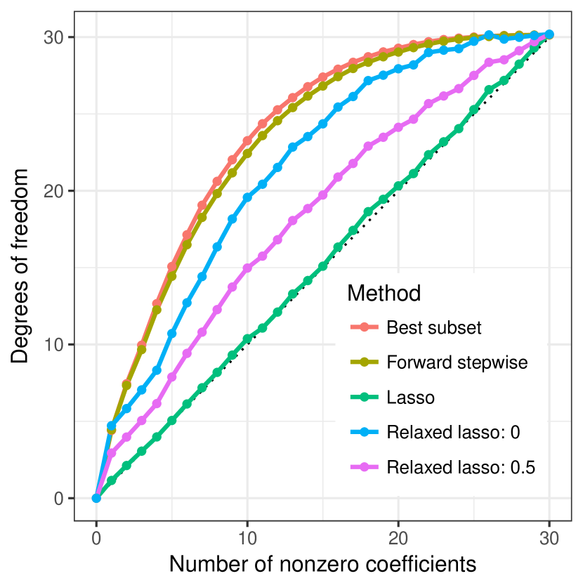
Figure 1 uses the latter perspective of effective degrees of freedom to contrast the aggressiveness of the three methods.
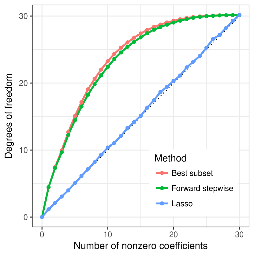
When the signal-to-noise ratio (SNR) is low, and also depending on other factors like the correlations between predictor variables, the more aggressive best subset and forward stepwise methods can already have quite high variance at the start of their model paths (i.e., for small step numbers ). Even after optimizing over the tuning parameter (using say, an external validation set or an oracle which reveals the true risk), we can arrive at an estimator with unwanted variance and worse accuracy than a properly tuned lasso estimator. On the other hand, for high SNR values, and other configurations for the correlations between predictors, etc., the story can be completely flipped and the shrinkage applied by the lasso estimator can result in unwanted bias and worse accuracy than best subset selection and forward stepwise selection. See Figure 2 for empirical evidence.
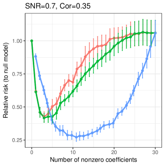
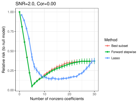
This is a simple point, but is worth emphasizing. To convey the idea once more:
Different procedures bring us from the high bias to the high variance ends of the tradeoff along different model paths; and these paths are affected by aspects of the problem setting, like the SNR and predictor correlations, in different ways. For some classes of problems, some procedures admit more fruitful paths, and for other classes, other procedures admit more fruitful paths. For example, neither best subset selection nor the lasso dominates the other, across all problem settings.
2.2 What is a realistic signal-to-noise ratio?
In their simulation studies, Bertsimas et al. (2016) considered SNRs in the range of about 2 to 8 in their low-dimensional cases, and about 3 to 10 in their high-dimensional cases. Is this a realistic range that one encounters in practice? In our view, inspecting the proportion of variance explained (PVE) can help to answer this question.
Let be a pair of predictor and response variables, and define and , so that we may express the relationship between as:
The signal-to-noise ratio (SNR) in this model is defined as
For a given prediction fuction —e.g., one trained on samples , that are i.i.d. to —its associated proportion of variance explained (PVE) is defined as
Of course, this is maximized when we take to be the mean function itself, in which case
In the second equality we have assumed independence of , so . As the optimal prediction function is , it sets the gold-standard of for the PVE, so we should always expect to see the attained PVE be less than and greater than 0 (otherwise we could simply replace our prediction function by .)
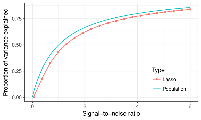
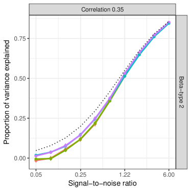
We illustrate using a simulation with and . The predictor autocorrelation was zero and the coefficients followed the beta-type 2 pattern with ; see Section 3.1 for details. We varied the SNR in the simulation from 0.05 to 6 in 20 equally spaced values. We computed the lasso over 50 values of the tuning parameter , and selected the tuning parameter by optimizing prediction error on a separate validation set of size . Figure 3 shows the PVE of the tuned lasso estimator, averaged over 20 repetitions from this simulation setup. Also shown is the population PVE, i.e., the maximum possible PVE at any given SNR level, of . We see that an SNR of 1.0 corresponds to a PVE of about 0.45 (with a maximum of 0.5), while an SNR as low as 0.25 yields a PVE of 0.1 (with a maximum of 0.2). In our experience, a PVE of 0.5 is rare for noisy observational data, and 0.2 may be more typical. A PVE of 0.86, corresponding to an SNR of 6, is unheard of! With financial returns data, explaining even 2% of the variance (PVE of 0.02) would be considered huge, and the corresponding prediction function could lead to considerable profits if used in a trading scheme. Therefore, based on these observations, we examine a wider lower range of SNRs in our simulations, compared to the SNRs studied in Bertsimas et al. (2016).
2.3 A (simplified) relaxed lasso
In addition to the lasso estimator, we consider a simplified version of the relaxed lasso estimator as originally defined by Meinshausen (2007). Let denote the solution in problem (4), i.e., the lasso estimator at the tuning parameter value . Let denote its active set, and let denote the least squares coefficients from regressing of on , the submatrix of active predictors. Finally, let be the full-sized (-dimensional) version of the least squares coefficients, padded with zeros in the appropriately. We consider the estimator defined by
| (7) |
with respect to the pair of tuning parameter values and . Recall (Tibshirani, 2013) that when the columns of are in general position (a weak condition occurring almost surely for continuously distributed pedictors, regardless of ), it holds that:
-
•
the lasso solution is unique;
-
•
the submatrix of active predictors has full column rank, thus is well-defined;
-
•
the lasso solution can be written (over its active set) as , where contains the signs of the active lasso coefficients.
Thus, under the general position assumption on , the simplified relaxed lasso can be rewritten as
| (8) | ||||
so we see that acts as a multiplicative factor applied directly to the “extra” shrinkage term apparent in the lasso coefficients. Henceforth, we will drop the word “simplified” and will just refer to this estimator as the relaxed lasso.
The relaxed lasso tries to undo the shrinkage inherent in the lasso estimator, to a varying degree, depending on . In this sense, we would expect it to be more aggressive than the lasso, and have a larger effective degrees of freedom. However, even in its most aggressive mode, , it is typically less aggressive than both forward stepwise selection and best subset selection, in that it often has a smaller degrees of freedom than these two. See Figure 4 for an example.
2.4 Other estimators
Many other sparse estimators for regression could be considered, for example, -penalized alternatives to the lasso, like the Dantzig selector (Candes and Tao, 2007) and square-root lasso (Belloni et al., 2011); greedy alternatives to forward stepwise algorithm, like matching pursuit (Mallat and Zhang, 1993) and orthogonal matching pursuit (Davis et al., 1994); nonconvex-penalized methods, such as SCAD (Fan and Li, 2001), MC+ (Zhang, 2010), and SparseNet (Mazumder et al., 2011); hybrid lasso/stepwise approaches like FLASH (Radchenko and James, 2011); and many others.
It would be interesting to include all of these estimators in our comparisons, though that would make for a huge simulation suite and would dilute the comparisons between best subset selection, forward stepwise, and the lasso that we would like to highlight. Roughly speaking, we would expect the Dantzig selector and square-root lasso to perform similarly to the lasso; the matching pursuit variants to perform similarly to forward stepwise; and the nonconvex-penalized methods to perform somewhere in between the lasso and best subset selection. (It is worth noting that our R package is structured in such a way to make further simulations and comparisons straightforward. We invite interested readers to use it to perform comparisons to other methods.)
2.5 Brief discussion of computational costs
Computation of the lasso solution in (4) has been a popular topic of research, and there are by now many efficient lasso algorithms. In our simulations, we use coordinate descent with warm starts over a sequence of tuning parameter values , as implemented in the glmnet R package (Friedman et al., 2007, 2010). The base code for this is written in Fortran, and warm starts—plus additional tricks like active set optimization and screening rules (Tibshirani et al., 2012)—make this implementation highly efficient. For example, for a problem with observations and variables, glmnet delivers the lasso solutions across 100 values of in less than 0.01 seconds, on a standard laptop computer. The relaxed lasso in (7) comes at only a slight increase in computational cost, seeing as we must only additionally compute the least squares coefficients on each active set. We provide an implementation in the bestsubset R package accompanying this paper, which just uses an R wrapper around glmnet. For the same example with and , computing the relaxed lasso path over 100 values of and 10 values of again took less than 0.01 seconds.
For forward stepwise selection, we implemented our own version in the bestsubset R package. The core matrix manipulations for this method are written in C, and the rest is written in R. The forward stepwise path is highly structured and this greatly aids its computation: at step , we have active variables included in the model, and we seek the variable among the remaining that—once orthogonalized with respect to the current active set of variables—achieves the greatest absolute correlation with , as in (2). Suppose that we have maintained a QR decomposition of the active submatrix of predictors, as well as the orthogonalization of the remaining predictors with respect to . We can compute the necessary correlations in operations, update the QR factorization of in constant time, and orthogonalize the remaining predictors with respect to the one just included in operations (refer to the modified Gram-Schmidt algorithm in Golub and Van Loan 1996). Hence, the forward stepwise selection path can be seen as a certain guided QR decomposition for computing the least squares coefficients on all variables (or, on some subset of variables when ). For the same example with and , our implementation computes the forward stepwise path in less than 0.5 seconds.
Best subset selection (1) is the most computationally challenging, by a large margin. Bertsimas et al. (2016) describe two reformulations of (1) as a mixed integer quadratic program, one that is preferred when , and the other when , and recommend using the Gurobi commercial MIO solver (which is free for academic use). They also describe a proximal gradient descent method for computing approximate solutions in (1), and recommend using the best output from this algorithm over many randomly-initialized runs to warm start the Gurobi solver. See Bertsimas et al. (2016) for details. We have implemented the method of these authors222We thank the third author Rahul Mazumder for his help and guidance.—which transforms the best subset selection problem into one of two MIO formulations depending on the relative sizes of and , uses proximal gradient to compute a warm start, and then calls Gurobi through its R interface—in our accompanying R package bestsubset.
Gurobi uses branch-and-cut techniques (a combination of branch-and-bound and cutting plane methods), along with many other sophisticated optimization tools, for MIO problems. Compared to the pure branch-and-bound method from the leaps R package, its speed can be impressive: for example, in one run with and , it returned the best subset selection solution of size in about 3 minutes (brute-force search for this problem would need to have looked at about 186 billion candidates!). But for most problems of this size ( and ) it has been our experience that Gurobi typically requires 1 hour or longer to complete its optimization. The third author Rahul Mazumder of Bertsimas et al. (2016) suggested to us that for these problem sizes, it is often the case that Gurobi has found the solution in less than 3 minutes, though it takes much longer to certify its optimality. For our simulations in the next section, we used a time limit of 3 minutes for Gurobi to optimize the best subset selection problem (1) at any particular value of the subset size (once the time limit has been reached, the solver returns its best iterate). For more discussion on this choice and its implications, see Section 3.2. We note that this is already quite a steep computational cost for “regular” practical usage: at 3 minutes per value of , if we wanted to use 10-fold cross-validation to choose between the subset sizes , then we are already facing 25 hours of computation time.
3 Simulations
3.1 Setup
We present simulations, basically following the simulation setup of Bertsimas et al. (2016), except that we consider a wider range of SNR values. Given (problem dimensions), (sparsity level), beta-type (pattern of sparsity), (predictor autocorrelation level), and (SNR level), our process can be described as follows:
-
i.
we define coefficients according to and the beta-type, as described below;
-
ii.
we draw the rows of the predictor matrix i.i.d. from , where has entry equal to ;
-
iii.
we draw the response vector from , with defined to meet the desired SNR level, i.e., ;
-
iv.
we run the lasso, relaxed lasso, forward stepwise selection, and best subset selection on the data , each over a wide range of tuning parameter values; for each method we choose the tuning parameter by minimizing prediction error on validation set that is generated independently of and identically to , as in steps ii–iii above;
-
v.
we record several metrics of interest, as specified below;
-
vi.
we repeat steps ii-v a total of 10 times, and average the results.
Below we describe some aspects of the simulation process in more detail.
Coefficients.
We considered four settings for the coefficients :
-
•
beta-type 1: has components equal to 1, occurring at (roughly) equally-spaced indices between 1 and , and the rest equal to 0;
-
•
beta-type 2: has its first components equal to 1, and the rest equal to 0;
-
•
beta-type 3: has its first components taking nonzero values equally-spaced between 10 and 0.5, and the rest equal to 0;
-
•
beta-type 5: has its first components equal to 1, and the rest decaying exponentially to 0, specifically, , for .
The first three types were studied in Bertsimas et al. (2016). They also defined a fourth type that we did not include here, as we found it yielded basically the same results as beta-type 3. The last type above is new: we included it to investigate the effects of weak sparsity and call it beta-type 5, to avoid confusion.
Evaluation metrics.
Let denote test predictor values drawn from (as in the rows of the training predictor matrix ) and let denote its associated response value drawn from . Also let denote estimated coefficients from one of the regression procedures. We considered the following evaluation metrics:
-
•
Relative risk: this is the accuracy metric studied in Bertsimas et al. (2016)333Actually, these authors used an “in-sample” version of this metric defined as , whereas our definition is “out-of-sample”, with an expectation over the new test predictor value taking the place of the sample average over the training values , ., defined as
The expectations here and below are taken over the test point , with all training data and validation data (and thus ) held fixed. A perfect score is 0 (if ) and the null score is 1 (if ).
-
•
Relative test error: this measures the expected test error relative to the Bayes error rate,
A perfect score is 1 and the null score is .
-
•
Proportion of variance explained: as defined in Section 2.2, this is
A perfect score is and the null score is 0.
-
•
Number of nonzeros: unlike the last three metrics which measure predictive accuracy, this metric simply records the number of nonzero estimated coefficients, .
It is worth noting that, in addition to metrics based on predictive accuracy, it would be useful to consider a metric that measures proper variable recovery, i.e., the extent to which the sparsity pattern in the estimated matches that in . We briefly touch on this in the discussion. Here we mention one advantage to studying predictive accuracy: any of the metrics defined above are still relevant when is no longer assumed to be linear, making the predictive angle more broadly practically relevant than a study of proper variable recovery (which necessarily requires linearity of the true mean).
Configurations.
We considered the following four problem settings:
-
•
low: , , ;
-
•
medium: , , ;
-
•
high-5: , , ;
-
•
high-10: , , .
In each setting, we considered ten values for the SNR ranging from 0.05 to 6 on a log scale, namely
(For convenience we provide the corresponding population PVE as well.) In each setting, we also considered three values for the predictor autocorrelation , namely 0, 0.35, and 0.7.
Tuning of procedures.
In the low setting, the lasso was tuned over 50 values of ranging from to a small fraction of on a log scale, as per the default in glmnet, and the relaxed lasso was tuned over the same 50 values of , and 10 values of equally spaced from 1 to 0 (hence a total of 500 tuning parameter values). Also in the low setting, forward stepwise and best subset selection were tuned over steps . In all other problem settings (medium, high-5, and high-10), the lasso was tuned over 100 values of , the relaxed lasso was tuned over the same 100 values of and 10 values of (hence 1000 tuning parameter values total), and forward stepwise and best subset selection were tuned over steps . In all cases, tuning was performed by by minimizing prediction error on an external validation set of size , which we note approximately matches the precision of leave-one-out cross-validation.
3.2 Time budget for Gurobi
As mentioned in Section 2.5, for each problem instance and subset size , we used a time limit of 3 minutes for Gurobi to optimize the best subset selection problem. In comparison, Bertsimas et al. (2016) used much larger time budgets: 15 minutes (per problem per ) for problems with as in our medium setup, and 66 minutes (per problem per ) for problems with as in our high-5 and high-10 setups. Their simulations however were not as extensive, as they looked at fewer combinations of beta-types, SNR levels, and correlation levels. Another important difference worth mentioning: the Gurobi optimizer, when run through its Python/Matlab interface, as in Bertsimas et al. (2016), automatically takes advantage of multithreading capabilities; this does not appear to be the case when run through its R interface, as in our simulations.
The third author of Bertsimas et al. (2016), Rahul Mazumder, suggested in personal communication that the MIO solver in the medium setting will often arrive at the best subset selection solution in less than 3 minutes, but it can take much longer to certify its optimality444Gurobi constructs a sequence of lower and upper bounds on the criterion in (1); typically the lower bounds come from convex relaxations and the upper bounds from the current iterates, and it is the lower bounds that take so long to converge. (usually over 1 hour, in absence of extra speedup tricks as described in Bertsimas et al., 2016). Meanwhile, in the high-5 and high-10 settings, this author also pointed out that 3 minutes may no longer be enough. For practical reasons, we have kept the 3 minute budget per problem instance per subset size. Note that this amounts to 150 minutes per path of 50 solutions, 1500 minutes or 25 hours per set of 10 repetitions, and in total 750 hours or 31.25 days for any given setting, once we go through the 10 SNR levels and 3 correlation levels.
3.3 Results: computation time
In Table 1, we report the time in seconds taken by each method to compute one path of solutions, averaged over 10 repetitions and all SNR and predictor correlation levels in the given setting. All timings were recorded on a Linux cluster. As explained above, the lasso path consisted of 50 tuning parameter values in the low setting and 100 in all other settings, the relaxed lasso path consisted of 500 tuning parameter values in the low setting and 1000 in all other settings, and the forward stepwise and best subset selection paths each consisted of tuning parameter values.
| Setting | BS | FS | Lasso | RLasso |
|---|---|---|---|---|
| low (, , ) | 3.43 | 0.006 | 0.002 | 0.002 |
| medium (, , ) | min | 0.818 | 0.009 | 0.009 |
| high-5 (, , ) | min | 0.137 | 0.011 | 0.011 |
| high-10 (, , ) | min | 0.277 | 0.019 | 0.021 |
We can see that the lasso and relaxed lasso are very fast, requiring less than 25 milliseconds in every case. Forward stepwise selection is also fast, though not quite as fast as the lasso (some of the differences here might be due to the fact that our forward stepwise algorithm is implemented partly in R). Moreover, it should be noted that when and is large, and one wants to explore models with a sizeable number of variables (we limited our search to models of size 50), forward stepwise has to plod through its path one variable at a time, but the lasso can make jumps over subset sizes bigger than one by varying and leveraging warm starts.
Recall, the MIO solver for best subset selection was allowed 3 minutes per subset size , or 150 minutes for a path of 50 subset sizes. As the times in Table 1 suggest, the maximum allotted time was not reached in all instances, and the MIO solver managed to verify optimality of some solutions along the path. In the medium setting, on average 17.55 of the 50 solutions were verified as being optimal. In the high-5 and high-10 settings, only 1.61 of the 50 were verified on average (note this count includes the subset of size 1, which is trivial). These measures may be pessismistic, as Gurobi may have found high-quality approximate solutions or even exact solutions but was just not able to verify them in time, see the discussion in the above subsection.
3.4 Results: accuracy metrics
Here we display a slice of the accuracy results, focusing for concreteness on the case in which the predictor autocorrelation is , and the population coefficients follow the beta-type 2 pattern. In a supplementary document, we display the full set of results, over the whole simulation design.
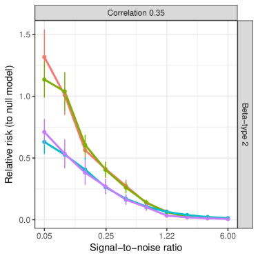
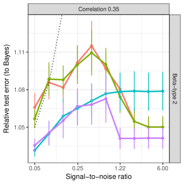
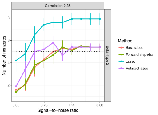
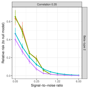
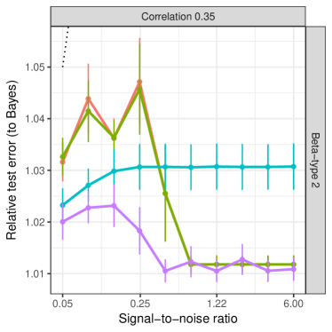
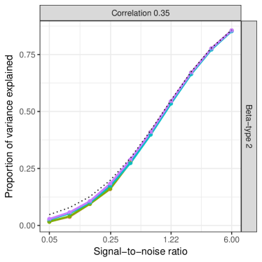
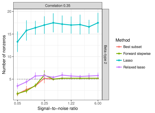
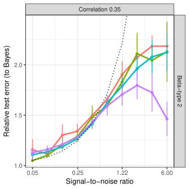
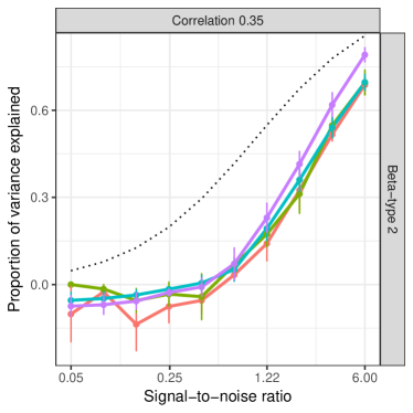
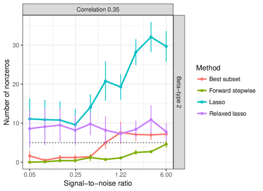
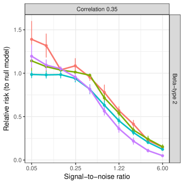
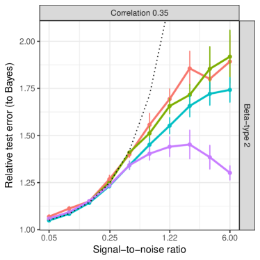
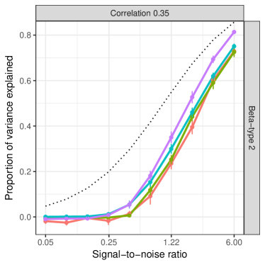
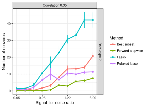
Figure 5 plots the relative risk, relative test error, PVE, and number of nonzero coefficients as functions of the SNR level, for the low setting. Figures 6, 7, and 8 show the same for the medium, high-5, and high-10 settings, respectively. Each panel in the figures displays the average of a given metric over 10 repetitions, for the four methods in question, and vertical bars denote one standard error. In the relative test error plots, the dotted curve denotes the performance of the null model (null score); in the PVE plots, it denotes the performance of the true model (perfect score); in the number of nonzero plots, it marks the true support size .
The low and medium settings, Figures 5 and 6, yield somewhat similar results. In the relative risk and PVE plots (top left and bottom left panels), we see that best subset and forward stepwise selection lag behind the lasso and relaxed lasso in terms of accuracy for low SNR levels, and as the SNR increases, we see that all four methods converge to nearly perfect accuracy. The relative test error plot (top right panel) magnifies the differences between the methods. For low SNR levels, we see that the lasso outperforms the more aggressive best subset and forward stepwise methods, but for high SNR levels, it is outperformed by the latter two methods. The critical transition point—the SNR value at which their relative test error curves cross—is different for the low and medium settings: for the low setting, it is around 1.22, and for the medium setting, it is earlier, around 0.42. The relaxed lasso, meanwhile, is competitive across all SNR levels: at low SNR levels it matches the performance of the lasso at low SNR levels, and at high SNR levels it matches that of best subset and forward stepwise selection. It is able to do so by properly tuning the amount of shrinkage (via its parameter ) on the validation set. Lastly, the number of nonzero estimated coefficients from the four methods (bottom right panel) is also revealing. The lasso consistently delivers much denser solutions; essentially, to optimize prediction error on the validation set, it is forced to do so, as the sparser solutions along its path feature too much shrinkage. The relaxed lasso does not suffer from this issue, again thanks to its ability to unshrink (move away from 1); it delivers solutions that are just as sparse as those from best subset and forward stepwise selection, except at the low SNR range.
The high-5 and high-10 settings, Figures 7 and 8, behave quite differently. The high-5 setting (smaller and smaller ) is more dire: the PVEs delivered by all methods—especially best subset selection—are negative for low SNR values, due to poor tuning on the validation set (had we chosen the null model for each method, the PVE would have been zero). In both the high-5 and high-10 settings, we see that there is generally no reason, based on relative risk, relative test error, or PVE, to favor best subset selection or forward stepwise selection over the lasso. At low SNR levels, best subset and forward stepwise selection often have worse accuracy metrics (and certainly more erratic metrics); at high SNR levels, these procedures do not show much of an advantage. For best subset selection, it is quite possible that its performance at the high SNR range would improve if we gave Gurobi a greater budget (than 3 minutes per problem instance per subset size). The relaxed lasso again performs the best overall, with a noticeable gap in performance at the high SNR levels. As is confirmed by the number of nonzero coefficients plots, the lasso and best subset/forward stepwise selection achieve similar accuracy in the high SNR range using two opposite strategies: the former uses high-bias and low-variance estimates, and the latter uses low-bias and high-variance estimates. The relaxed lasso is most accurate by striking a favorable balance between these two polar regimes.
Low setting: , ,
Correlation , beta-type 2
 |
 |
 |
 |
Medium setting: , ,
Correlation , beta-type 2
 |
 |
 |
 |
High-5 setting: , ,
Correlation , beta-type 2
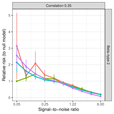 |
 |
 |
 |
High-10 setting: , ,
Correlation , beta-type 2
 |
 |
 |
 |
3.5 Summary of results
As mentioned above, the results from our entire simulation suite can be found in a supplementary document. Here is a high-level summary.
-
•
An important caveat to emphasize upfront is that the Gurobi MIO algorithm for best subset selection was given 3 minutes per problem instance per subset size. This practical restriction may have caused best subset selection to underperform, in particular, at the high SNR levels in the high-5 and high-10 settings.
-
•
Forward stepwise selection and best subset selection perform quite similarly throughout (with the former being much faster). This does not agree with the results for forward stepwise in Bertsimas et al. (2016), where it performed quite poorly in comparison. In talking with the third author, Rahul Mazumder, we have learned that this was due to the fact that forward stepwise in their study was tuned using AIC, rather than a separate validation set. So, when put on equal footing and allowed to select its tuning parameter using validation data just as the other methods, we see that it performs quite comparably.
-
•
The lasso gives better accuracy results than best subset selection in the low SNR range and worse accuracy than best subset in the high SNR range. The transition point—the SNR level past which best subset outperforms the lasso—varies depending on the problem dimensions () predictor autocorrelation (), and beta-type (1 through 5). For the medium setting, the transition point comes earlier than in the low setting. For the high-5 and high-10 settings, the transition point often does not come at all (before an SNR of 6, which is the maximum value we considered). As the predictor autocorrelation level increases, the transition point typically appears later (again, in some cases it does not come at all, e.g., for beta-type 5 and autocorrelation ).
-
•
The relaxed lasso provides altogether the top accuracy results. In nearly all cases (across all SNR levels, and in all problem configurations) we considered, it performs as well as or better than all other methods. We conclude that it is able to use its auxiliary shrinkage parameter () to get the “best of both worlds”: it accepts the heavy shrinkage from the lasso when such shrinkage is helpful, and reverses it when it is not.
-
•
The proportion of variance explained plots remind us that, despite what may seem like large relative differences, the four methods under consideration do not have very different absolute performances in this intuitive and important metric. It thus makes sense overall to favor the methods that are easy to compute.
4 Discussion
The recent work of Bertsimas et al. (2016) has enabled the first large-scale empirical examinations of best subset selection. In this paper, we have expanded and refined the simulations in their work, comparing best subset selection to forward stepwise selection, the lasso, and the relaxed lasso. We have found: (a) forward stepwise selection and best subset selection perform similarly throughout; (b) best subset selection often loses to the lasso except in the high SNR range; (c) the relaxed lasso achieves “the best of both worlds” and performs on par with the best method in each scenario. We note that these comparisons are based on (various measures of) out-of-sample prediction accuracy. A different target, e.g., a measure of support recovery, may yield different results.
Our R package bestsubset, designed to easily replicate all of the simulations in this work, or forge new comparisons, is available at https://github.com/ryantibs/best-subset/.
References
- (1)
- Beale et al. (1967) Beale, E. M. L., Kendall, M. G. and Mann, D. W. (1967), ‘The discarding of variables in multivariate analysis’, Biometrika 54(3/4), 357–366.
- Belloni et al. (2011) Belloni, A., Chernozhukov, V. and Wang, L. (2011), ‘Square-root lasso: pivotal recovery of sparse signals via conic programming’, Biometrika 98(4), 791–806.
- Bertsimas et al. (2016) Bertsimas, D., King, A. and Mazumder, R. (2016), ‘Best subset selection via a modern optimization lens’, The Annals of Statistics 44(2), 813–852.
- Candes and Tao (2007) Candes, E. J. and Tao, T. (2007), ‘The Dantzig selector: statistical estimation when is much larger than ’, Annals of Statistics 35(6), 2313–2351.
- Chen et al. (1998) Chen, S., Donoho, D. L. and Saunders, M. (1998), ‘Atomic decomposition for basis pursuit’, SIAM Journal on Scientific Computing 20(1), 33–61.
- Davis et al. (1994) Davis, G., Mallat, S. and Zhang, Z. (1994), ‘Adaptive time-frequency decompositions with matching pursuit’, Wavelet Applications 402, 402–413.
- Draper and Smith (1966) Draper, N. and Smith, H. (1966), Applied Regression Analysis, Wiley.
- Efron et al. (2004) Efron, B., Hastie, T., Johnstone, I. and Tibshirani, R. (2004), ‘Least angle regression’, Annals of Statistics 32(2), 407–499.
- Efroymson (1966) Efroymson, M. (1966), ‘Stepwise regression—a backward and forward look’, Eastern Regional Meetings of the Institute of Mathematical Statistics .
- Fan and Li (2001) Fan, J. and Li, R. (2001), ‘Variable selection via nonconcave penalized likelihood and its oracle properties’, Journal of the American Statistical Association 96(456), 1348–1360.
- Friedman et al. (2007) Friedman, J., Hastie, T., Hoefling, H. and Tibshirani, R. (2007), ‘Pathwise coordinate optimization’, Annals of Applied Statistics 1(2), 302–332.
- Friedman et al. (2010) Friedman, J., Hastie, T. and Tibshirani, R. (2010), ‘Regularization paths for generalized linear models via coordinate descent’, Journal of Statistical Software 33(1), 1–22.
- Furnival and Wilson (1974) Furnival, G. and Wilson, R. (1974), ‘Regression by leaps and bounds’, Technometrics 16(4), 499–511.
- Golub and Van Loan (1996) Golub, G. H. and Van Loan, C. F. (1996), Matrix computations, The Johns Hopkins University Press. Third edition.
- Hastie et al. (2009) Hastie, T., Tibshirani, R. and Friedman, J. (2009), The Elements of Statistical Learning; Data Mining, Inference and Prediction, Springer. Second edition.
- Hocking and Leslie (1967) Hocking, R. R. and Leslie, R. N. (1967), ‘Selection of the best subset in regression analysis’, Technometrics 9(4), 531–540.
- Janson et al. (2015) Janson, L., Fithian, W. and Hastie, T. (2015), ‘Effective degrees of freedom: A flawed metaphor’, Biometrika 102(2), 479–485.
- Kaufman and Rosset (2014) Kaufman, S. and Rosset, S. (2014), ‘When does more regularization imply fewer degrees of freedom? Sufficient conditions and counterexamples’, Biometrika 101(4), 771–784.
- Mallat and Zhang (1993) Mallat, S. and Zhang, Z. (1993), ‘Matching pursuits with time-frequency dictionaries’, IEEE Transactions on Signal Processing 41(12), 3397–3415.
- Mazumder et al. (2011) Mazumder, R., Friedman, J. and Hastie, T. (2011), ‘SparseNet: Coordinate descent with nonconvex penalties’, Journal of the American Statistical Association 106(495), 1125–1138.
- Meinshausen (2007) Meinshausen, N. (2007), ‘Relaxed lasso’, Computational Statistics & Data Analysis 52, 374–393.
- Natarajan (1995) Natarajan, B. K. (1995), ‘Sparse approximate solutions to linear systems’, SIAM Journal on Computing 24(2), 227–234.
- Radchenko and James (2011) Radchenko, P. and James, G. M. (2011), ‘Improved variable selection with forward-lasso adaptive shrinkage’, The Annals of Applied Statistics 5(1), 427–448.
- Tibshirani (1996) Tibshirani, R. (1996), ‘Regression shrinkage and selection via the lasso’, Journal of the Royal Statistical Society: Series B 58(1), 267–288.
- Tibshirani et al. (2012) Tibshirani, R., Bien, J., Friedman, J., Hastie, T., Simon, N., Taylor, J. and Tibshirani, R. J. (2012), ‘Strong rules for discarding predictors in lasso-type problems’, Journal of the Royal Statistical Society: Series B 74(2), 245–266.
- Tibshirani (2013) Tibshirani, R. J. (2013), ‘The lasso problem and uniqueness’, Electronic Journal of Statistics 7, 1456–1490.
- Tibshirani and Taylor (2012) Tibshirani, R. J. and Taylor, J. (2012), ‘Degrees of freedom in lasso problems’, Annals of Statistics 40(2), 1198–1232.
- Zhang (2010) Zhang, C.-H. (2010), ‘Nearly unbiased variable selection under minimax concave penalty’, The Annals of Statistics 38(2), 894–942.
- Zou et al. (2007) Zou, H., Hastie, T. and Tibshirani, R. (2007), ‘On the “degrees of freedom” of the lasso’, Annals of Statistics 35(5), 2173–2192.
Supplement to “Extended Comparisons of Best Subset Selection, Forward Stepwise Selection, and the Lasso”
This supplementary document contains plots from the simulation suite described in the paper “Extended Comparisons of Best Subset Selection, Forward Stepwise Selection, and the Lasso”. The plots in Section 1 precisely follow the simulation format described in the paper. Those in Section 2 follow an analogous format, except that the tuning has been done using an “oracle”, rather than a validation set as in Section 1. Specifically, the tuning parameter for each method in each scenario is chosen to minimize the average risk over all of the repetitions.
.tocapp \etocsettagdepthmainnone \etocsettagdepthappsubsubsection
Appendix A Validation tuning
A.1 Low setting: , ,
A.1.1 Relative risk (to null model)
![[Uncaptioned image]](/html/1707.08692/assets/x22.png)
A.1.2 Relative test error (to Bayes)
![[Uncaptioned image]](/html/1707.08692/assets/x23.png)
A.1.3 Proportion of variance explained
![[Uncaptioned image]](/html/1707.08692/assets/x24.png)
A.1.4 Number of nonzero coefficients
![[Uncaptioned image]](/html/1707.08692/assets/x25.png)
A.2 Medium setting: , ,
A.2.1 Relative risk (to null model)
![[Uncaptioned image]](/html/1707.08692/assets/x26.png)
A.2.2 Relative test error (to Bayes)
![[Uncaptioned image]](/html/1707.08692/assets/x27.png)
A.2.3 Proportion of variance explained
![[Uncaptioned image]](/html/1707.08692/assets/x28.png)
A.2.4 Number of nonzero coefficients
![[Uncaptioned image]](/html/1707.08692/assets/x29.png)
A.3 High-5 setting: , ,
A.3.1 Relative risk (to null model)
![[Uncaptioned image]](/html/1707.08692/assets/x30.png)
A.3.2 Relative test error (to Bayes)
![[Uncaptioned image]](/html/1707.08692/assets/x31.png)
A.3.3 Proportion of variance explained
![[Uncaptioned image]](/html/1707.08692/assets/x32.png)
A.3.4 Number of nonzero coefficients
![[Uncaptioned image]](/html/1707.08692/assets/x33.png)
A.4 High-10 setting: , ,
A.4.1 Relative risk (to null model)
![[Uncaptioned image]](/html/1707.08692/assets/x34.png)
A.4.2 Relative test error (to Bayes)
![[Uncaptioned image]](/html/1707.08692/assets/x35.png)
A.4.3 Proportion of variance explained
![[Uncaptioned image]](/html/1707.08692/assets/x36.png)
A.4.4 Number of nonzero coefficients
![[Uncaptioned image]](/html/1707.08692/assets/x37.png)
Appendix B Oracle tuning
B.1 Low setting: , ,
B.1.1 Relative risk (to null model)
![[Uncaptioned image]](/html/1707.08692/assets/x38.png)
B.1.2 Relative test error (to Bayes)
![[Uncaptioned image]](/html/1707.08692/assets/x39.png)
B.1.3 Proportion of variance explained
![[Uncaptioned image]](/html/1707.08692/assets/x40.png)
B.1.4 Number of nonzero coefficients
![[Uncaptioned image]](/html/1707.08692/assets/x41.png)
B.2 Medium setting: , ,
B.2.1 Relative risk (to null model)
![[Uncaptioned image]](/html/1707.08692/assets/x42.png)
B.2.2 Relative test error (to Bayes)
![[Uncaptioned image]](/html/1707.08692/assets/x43.png)
B.2.3 Proportion of variance explained
![[Uncaptioned image]](/html/1707.08692/assets/x44.png)
B.2.4 Number of nonzero coefficients
![[Uncaptioned image]](/html/1707.08692/assets/x45.png)
B.3 High-5 setting: , ,
B.3.1 Relative risk (to null model)
![[Uncaptioned image]](/html/1707.08692/assets/x46.png)
B.3.2 Relative test error (to Bayes)
![[Uncaptioned image]](/html/1707.08692/assets/x47.png)
B.3.3 Proportion of variance explained
![[Uncaptioned image]](/html/1707.08692/assets/x48.png)
B.3.4 Number of nonzero coefficients
![[Uncaptioned image]](/html/1707.08692/assets/x49.png)
B.4 High-10 setting: , ,
B.4.1 Relative risk (to null model)
![[Uncaptioned image]](/html/1707.08692/assets/x50.png)
B.4.2 Relative test error (to Bayes)
![[Uncaptioned image]](/html/1707.08692/assets/x51.png)
B.4.3 Proportion of variance explained
![[Uncaptioned image]](/html/1707.08692/assets/x52.png)
B.4.4 Number of nonzero coefficients
![[Uncaptioned image]](/html/1707.08692/assets/x53.png)