Change Point Detection with Optimal Transport and Geometric Discrepancy
Abstract
We present novel retrospective change point detection approach based on optimal transport and geometric discrepancy. The method does not require any parametric assumptions about distributions separated by change points. It can be used both for single and multiple change point detection and estimation, while the number of change points is either known or unknown. This result is achieved by construction of a certain sliding window statistic from which change points can be derived with elementary convex geometry in a specific Hilbert space. The work is illustrated with computational examples, both artificially constructed and based on actual data.
Introduction
Change point problem was firstly mentioned by Stewhart [28] as a problem of industrial quality control in the year 1928. This problem was solved by Girshick and Rubin [10] in 1953. The optimal solutions for parametric online formulation of the problem were provided by Shiryaev and Pollak [29],[25]. Asymptotically optimal posteriori change point detection method was developed by Borovkov [2]. This method requires knowledge of parametric likelihood functions, however it can be translated to nonparametric case with empirical likelihood [15]. The fundamental results in nonparametric study of change-point problem are due Brodsky and Darkhovsky [3], and Horvath et al. [6]. These methods are generally tailored for one-dimensional data. Nonparametric change point inference with multidimensional data is still an open problem. New methods are still being developed usually with applications of ideas from other scopes to change point data. For example, [21], where divergence from cluster network analysis is used in order to estimate both the number and the locations of change points or [20], where multivariate version of Wilcoxon rank statistic is computed.
This work is focused on nonparametric change point detection in multivariate data. This problem has large scope of applications including finance [31],genomics [23] and signal processing [16].
The problem of optimal transportation were introduced by Monge [22] in the year 1781. The modern statement of the problem is due to Kantorovich as it was stated in the seminal paper in 1941 [14]. We recommend [33] and [26] as modern references to the subject
Vector rank and quantile functions were introduced by Serfiling [27] as part Depth-Outlyingness-Quantile-Rank (DOQR) paradigm. Monge-kantorovich vector ranks were introduced by Chernozhukov et al. [4].
Study of discrepancy were started by H. Weyl [34] in 1916 with number theory as intended area of application, more computational aspects of discrepancy were pioneered by Niederreiter [24] (quasi- and pseudo- random number generation) and Hlawka [13] (numeric integration). We say that discrepancy is geometric when we talk about continuous distributions with fixed well-identified support, this is the opposition to the case of combinatorial discrepancy which study nonuniformity of finite distributions. The main contribution to the theory of quadratic generalized geometric discrepancy is by Hickernel [11]. This is a work of a highly synthetic nature. This Synthetic nature is coming from the combination of vector ranks and geometric discrepancy, optimal transport and change point problems. All this concepts are rarely to never seen together in scientific publications, however in this paper they are intertwined in a singular computational methodology.
But why these results come to existence only now? The answer to this questions in our case is rooted into the fact that computing discrepancy used to be computationally challenging task for non-uniform probability distributions. However, in the recent publication [4] by Chernozhukov,Carlie, Galichon and Halin the Monge-Kantorovich vector rank functions were introduced. Vector rank function can be understood in the context of this work as homeomorphic extension of classical one-dimensional cumulative distribution functions to multidimensional spaces. The idea of using low-discrepancy sequences as a tool for the estimation of the vector rank functions was already present in the [4]. As the name suggests discrepancy is the natural measure of consistency of the sequence to be low-discrepancy sequence in the same way as the order statistic is the natural measure of the sequence to be ordered. Thus, as classical one-dimensional ranks and order statistic is used in the construction of the classical Kolmogorov-Smirnov and Crámer-Von Mizes tests of goodness-of-fit, the vector rank function and discrepancy can be used in order to construct natural extension of this tests in the multidimensional context.
Thus, the main objective of the work is the exploration of vector rank discrepancy as methodology for nonparametric high-dimensional statistic. We select change point problem as the test subject for this inquiry.
The strict measure theoretic approach mentioned above is strengthened in this work as we speak about probability measures instead of probability distributions and densities whenever is possible which contradicts current trends in the statistical science. This can be justified by convenience of understanding measures as points in certain multidimensional spaces bearing intrinsic geometric structure. On the other hand, we view all mathematical constructions in this work as theoretical prototypes of certain concrete algorithms ad data structures which can be implemented in order to solve practical tasks. Our approach to the problem is highly inspired by [19] and we use convex geometric intuition whenever possible.
acknowledgement
Underlying research was conducted during author’s work for master’s degree in ”Mathematical methods of Optimization and Stochastics” program in NRU Higher School of Economics, Moscow, Russia. Author wants to thank head of the program Vladimir Spokoiny, his scientific advisor Andrei Sobolevski for suggesting the research topic and support, Alexey Naumov and Maxim Panov for the discussion in IITP RAS; Yuri Yanovich,Alexandra Suvorikova , Elena Chernousova and Alexey Kroshnin for fruitful discussion at the IUM seminar.
Notation
This is notation for the use in the sequel.
is a -dimensional euclidean space with . is a unit interval and is a unit hypercube in . In line with Kolmogorov’s axiomatics triple is a probability space, and every observation as a random variable is assumed to be a Borel measurable map from to . For brevity denotes the whole probability measure structure .
Every random variable defines the probability measure that is referred to as the probability law of , where denotes a pushforward of the measure by . That is, for every Borel set it holds that . In this case the notation is used. In case is a random process over domain notation means that defines the hierarchical probability distribution system of as a whole. In this case for all the measure is the distribution of a single observation and is the joint distribution of and i.e. . means that is independently identically distributed sample (i.i.d) with probability law .
A set of all probability laws with finite first and second moments is denoted by . A subset of of probability measures absolutely continuous with respect to Lebesgue measure is denoted by . is the uniform distribution over . It is obvious that .In the sequel is assumed to be implicitly equipped with for each , which makes it into a probability space, and is equipped with the counting measure.
If is an sequence of random elements in some metric space with distance metric , when it is said that converges to in probability if for each it holds , which is denoted as . In case is not a measurable function for all the convergence in outer probability may be introduced and denoted by . Having the convergence in outer probability is equivalent to for all .
If is a discrete time ergodic process with convergence in probability,
| (1) |
for every bounded Lipschitz function , we say that is the weak limit distribution of .
Problem Formulation
In this section a brief review for common variations of change point problem is provided.
Ordered Set is associated with time. It is possible to discuss change point problem with continuous time [9]. However, this work deals only with case of discrete time. It is also possible to consider a change point detection for random fields [3].
Two main types of change point problem are offline and online detection. In offline detection is assumed to be a finite set of size . Without loss of generality, it is assumed that . Initial observations are treated as a time series indexed by . Firstly, we discuss the case of a single change point.
Definition 1.
The change point of is an unknown moment of time such that and . There are two possibilities. Firstly, both subsamples may be i.i.d with and . It is also possible to consider unknowns and to be ergodic weak limit distributions of and respectively.
Then offline single change point detection problem is a hypothesis test for versus for every possible estimate of having . Retrieving valid value of is a related problem which will be referred as a change point estimation.
Definition 2.
In case of multiple change points existence of up to change moments is assumed. In simpler formulation of problem value of is assumed to be known, while in more complicated one is also an object of estimation. As the previous variation the problem is a hypothesis test about distribution of samples where and for simplicity. The problem splits into multiple hypothesis tests for versus for all possible estimates of in case of known . For unknown the problem is structured around testing against for all estimates of where possible values of are constricted to some meaningful finite set.
For online change point problem as an ordered set, and can be thought as infinite times series unfolding in real time. In this case the goal is to identify change point as soon as possible which means using minimal amount of observations with . Branding every moment of time as a change point will achieve zero delay. However, this detection procedure is unacceptable as it achieves maximal false alarm rate. This means that change-point detection algorithm needs to be tuned in for minimal delay with fixed false alarm rate.
In a more theoretical framework a single change point can be considered, which implies that infinite set of observations with prior distribution can be used for detection. However, in more practical situation the stream of chanege ponts is considered, with only finite sample available for detection of .
Generally, methods of change point detection are focused on detection of change in such properties of statistical distributions as mean, variance and spectral density. The method presented in this work is focused on change in ergodic weak limit distribution of data. Which means that change in mean and variance must be detectable, although, change in spectral density is not. Moreover, changes restricted to such properties of distribution as median or higher moments also must be traceable. Another restriction of proposed solution is a demand for all measures to belong to .
Construction of proposed change point detection starts with offline single detection problem. We restrict our attention to models with i.i.d distributed observations along one side of change point. In order to give meaningful characteristic to point estimates of change point this problem can be reformulated as certain probabilistic game against Nature. Two sample spaces and with corresponding families of random variables and taking values in are assumed to exist. We assume that both families are intrinsically i.i.d which means that and and the same holds for . This means that both sample probability spaces can be decomposed as and such that for each the random variable depends only on . The common sample space is constructed by the rule
| (2) |
with -algebras generated by a set . Note, that the only possible probability distribution on the set is a Bernoulli distribution with a parameter . So probability measure on can be defined by , where is a natural injection defined by . Nature defines value of and distribution laws and . Random variables are constructed by letting . Then, nature generates sample of observations of , sorts it by , then erases values of which retains observable sample of . Observer either claims that there were no change point which leads to a victory in case or equivalently is too close to either or . Otherwise, the observer gives point-estimate of which can be converted to a classical change-point estimate .
This construction also can be understood as a Bayesian assumption , where stands for binomial distribution. However, the change point problem is a single element sample problem, which means that only minimal properties of the parameter can be inferred from the data. This does not change the problem except for treating as an estimate of the mean.
Obviously,the observer chooses strategy which maximizes chances of victory. This can be interpreted in terms of loses , which are equal to in case observer claims no change point and otherwise. Let in case the observer gives estimate when no real change point exists.
If one preserves while increasing the empirical distribution of will converge to a measure , the convex combination of measures. It possible to think of as contained inside one-dimensional interval embedded into the infinite-dimensional convex space of probability measures. In order to construct such measures from random variables we will use random mixing map in the sequel. Here and .
In order to propose the solution strategy for the change point problem we introduce vector rank function such that , a known reference distribution of simple structure. For our application is a uniform distribution over a unit hypercube . It was shown in [4] and [8] that , an estimate of , can be recovered from data without any parametric assumptions.
If data is i.i.d distributed with laws and on each side of change point, when figure 1 will exhibit relations between probability distribution laws discussed so far.
The diagram shows that application of vector rank function can be thought as a probabilist’s ”change of basis”. The pragmatic value for change point problem is in elimination of unknown distribution from the model.
It is obvious that the diagram depicted at fig. 1 commute. As the pushforward acts as a linear map of signed measures defined over two different measurable spaces. If and are measures, , is a measurable set and is a measurable function, then
Therefore, by linearity of the pushforward
Thus, the diagram is correct.
The real result of change-point estimation will depend on measurable difference between and . We introduce notion of Kullback-Leibler divergence in order to quantify this difference.
Definition 3.
Kullback-Leibler divergence between measures and admitting densities and and respectively is
Note that while they admit densities. Now we formulate a sufficient condition on that ensures that our transformations preserve divergence between distributions.
If is invertible almost everywhere , when Let be a random variable such that . Then, and by invertibility a.e. of distribution has density a.e. ; similar fact is also true for . Then,
Formulation of the method
In this chapter our approach to construction of the vector rank function’s estimates is presented. The main goal of This approach is the avoidance of approximation of the entire function . Note, that even the estimation that the aim of this task is actually not a precise estimation of values for each observation but a construction of an estimate that preserves the relative geometry of a sample along its change points.
The work [4] presents continuous, semidiscrete, and discrete methods of estimation of . The Implementation of change point detection discussed in this section is based solely on discrete approach. The reason behind this choice is computational simplicity.
Vector rank function in general can be understood as -almost surely homeomorphisms between supports of sample probability distribution and reference probability law of choice ( is defined almost everywhere and continuous with respect to subset topology, and admits similar continuous inverse existing almost everywhere ) , such that and both depth median and symmetries are preserved. This symmetries and the concept of depth median need to be additionally defined, which goes beyond of the scope of this paper. In our application uniform measure over unit hypercube is selected as the reference . In case the cumulutive distribution function (cdf) of is also the ’vector’ rank function of the probability distribution of .
The vector rank function is not unique in general. We use Monge-Kantarovich vector rank developed in [4], which is defined as optimal transport between and
Vector rank role of the optimal transport map can be intuitively justified by the equivalence of the above optimization problem to the maximization of the integral
where and stands for depth medians of distributions and respectively. Thus, the optimal transport preserves geometric properties of distribution which can be expressed by inner products of points relative to its center of symmetry. This is what is understood as the relative geometry of the data ,and what we try to preserve during vector rank estimation.
In this work we are focused on the discrete estimation of vector rank function. Let be an equidistributed sequence of points in . That is, for every Lipschitz continuous function defined on it holds
| (3) |
Then, for observations define , where
| (4) |
In case convergence in (3) is understood as convergence a.s or even as convergence in probability the sequence can be taken as an i.i.d sequence of random variables or as an ergodic process with a uniform weak limit distribution. However, this implementation is more suited for deterministic form of . Discrepancy can be understood as a natural measure of slackness of condition (3) for a fixed value of .
Classical (one-sided) geometric discrepancy of the sequence is described by the formula
| (5) |
Note that (5) admits representation for a certain function . This idea were used in [11] to introduce generalized quadratic discrepancy with supremum-norm replaced by a certain quadratic norm in a certain Sobolev Space. The result can be expressed as
| (6) |
where is the reproducing Hilbert kernel of the Sobolev space
| (7) |
with standing for a scale parameter and standing for a functional parameter with square-integrable derivative with and the value defined by
and is the ith Bernoulli polynomial. Note, that in case statistic (5) turns into Kolmogorov-Smirnov statistic and (6) turns into Cr/‘amer-Von Mizes statistic for uniform distribution test.
The function is a functional parameter defining exact form of the discrepancy. In this text we use star discrepancy produced by
and the centred discrepancy produced by selecting
The case of being a low-discrepancy sequence is a particularly well suited for our application.
Definition 4.
low-discrepancy sequence is a deterministic sequence in designed with a goal of minimizing value the for each natural number .
Definition above is rather informal. However, it is postulated firmly that for any low-discrepancy sequence property (3) holds and for any choice of and . Thus, the rate of convergence of can be understood as a measure of efficiency of a low-discrepancy sequence .
In our application we use Sobol sequence with grey code implementation. Sobol sequence were introduced by Sobol [30] and the grey code implementation is due [1]. Detailed investigation of the nature of this sequence goes beyond the scope of this work. However, any other low-discrepancy sequence can be used.
For a Sobol sequence value converges to zero as , where depends on implicitly. While convergence rate of discrepancy for a random uniform sequence is , for value of , which makes low-discrepancy sequence rather efficient. However, scrambling and effective dimension techniques can increase rate of convergence [12].
It can be established that the sequences and have no repeating values almost surely, As our data is assumed to come from atomless distributions. This means that the problem of finding Permutation in (4) is the optimal assignment problem. The Optimal assignment problem is the special case the linear programming, which can be solved in time by the Hungarian algorithm [17][32]. Amortizations based on applications of parallel programming can improve computation complexity to . Approximate algorithms can be used for faster computations, for example [7].
Note, that even if sample has an i.i.d distribution, then the resulting transport is not independent itself. However, the covariance of the elements is converging to zero as goes to infinity. Let be two indices less or equal to and be coordinate indices. As is assumed to be i.i.d, it follows that has a discrete uniform distribution over . Then,
so by bounding from above and below with equidistribution property of in the limit case
where is a uniform random variable on . Thus, the value converges to zero. As variance of converges to the variance of a standard uniform distribution on we will treat sample as uncorrelated in asymptotic context under assumption of i.i.d. distribution of .
It can be easily seen that that quadratic discrepancy admits a degenerate V-statistic representation with the kernel :
| (8) |
assuming sample of elements. Properties of V-statistic produces the asymptotic result
where and are non-zero eigenvalues of the integral operator defined by the relation
It can be shown that is in fact positive-semidefinite and trace-class, which means that all and that
Eigenvalues of can be approximated by a finite collection of numbers with Nyström method. As it was shown in [5] the twofold approximation of cdf of is possible for fixed natural numbers , and parameter :
| (9) |
This formula can be used for computing quantiles and critical values of with simple one-dimensional zero-seeking algorithm.
Case of A Single Change Point
In this chapter an approach for detecting a single change point is presented. We impose a model assumptions that for a fixed change point either satisfy or it does not exist . This value can be selected in a such way that and be used as a sliding window bandwidth defining a ’control chart’-like object which we refer to as diphoragram.
Definition 5.
empirical sliding diphoragram for change point data is defined by
and ideal sliding diphoragram by
for in range from to .
If is a continuous function, then as . With this condition discrepancy is a continuous function of data. So, convergence of vector ranks proved in [4] implies convergence of diphoragrams. Note, that with kernel representation charts admit a difference representation
From the computational standpoint this means that computation of the whole time-series and takes only quadratic time in number in observation. Moreover, if crisp optimal transport with low-discrepancy sequence is used in estimation of vector rank function, then , so all values can be precomputed.
For the application to the change point problem consider two increasing sequences of integers and such that for all are constructed. Then as are assumed to be independent and are also independent random variables.
Definition 6.
mean sliding discrepancy for set sample is computed by
Note, that the mean sliding discrepancy is not the same as the discrepancy of the whole sample. By independence, in case holds, as
where . Otherwise, there will be a sliding discrepancies sampled form the non-uniform data which goes to in probability as . So, the whole sum .
In case the single change point exists the statistic is expected to attain the minimal value at such moment of time when the empirical distribution of approaches the empirical distribution of the whole sample, as the empirical distribution of the whole sample is converging to the . Let
It is expected that the ratio of numbers of elements from both sides of change point in the subsample used in the computation of and in the whole sample are equal. This can be represented in the algebraic relation
where is the produced estimate of the change point. This provides the expression for the estimate
We accept for a fixed -level in case
| (10) |
where the cdf is numerically estimated as in (9) for some fixed parameters and . Otherwise reject and state that there was a change most probable at .
In order to reason about properties of the estimate . Let denote space of finite signed measures other the hypercube .
Definition 7.
Space of nonuniformities is defined as a quotient of the real vector spaces
endowed with a Hilbert space structure by inner product defined for by
| (11) |
Note, that the relation (11) is well defined as for all
as for any value of and is symmetric and is indeed an inner product as is a positive-definite kernel. As the line intersects simplex of probability measures only in one point ( itself) the natural projection is injective on , so we denote a nonuniformity arising from each just as . If every subsample is associated with an empirical measures , then
By construction of the vector rank function , hence in . This produces result
| (12) |
Considering that it follows that , so magnitude of the discrepancy will have the same distribution for sample with equal proportions of elements with distributions of and . If , then it can be shown that estimate is unbiased:
where
However, then the estimate is projected to be biased towards as the value will only increase and the value will only decrease as decreases. Otherwise, increase of increases the value too, and decreases the value of . In order to proof consistency of estimator we introduce a family of sequences for each
Then by the weak convergence of vector ranks for every the sequence converges to a value:
Otherwise . We can assert by structural uniformity of that in Skorohod’s topology. Thus, providing convergence in probability. This suggests that the bias of can be bounded by some sequence with convergence :
Without loss of generality assume that . Then, we separate positive bias into mixing and non-mixing parts:
For non-mixing part apply Markov inequality for each fixed value of and some value
It is possible to use inverse as for each . With this inequality the non-mixing part can be bounded
As with the rate it is possible to specify a constant in such a way that and the expectation approaches some constant value by weak convergence and therefore can be bounded. Thus, the non-mixing bias approaches zero as goes to infinity. Note, that all moments of discrepancy exists as it is bounded on a positive interval for each . This method can be extended in order to show that the estimate is asymptotically unbiased under an assumption of change point slackness,
Definition 8.
Sequence of diphoragrams has slackness property iff for some constant and for all large enough there are time points such that :
Then, it is possible to construct a similar bound
which converges to zero at infinity.
alternative methods
One of the negative properties of the method described in the previous chapter is the requirement of specification of bandwidth , which prevents change point detection in the proximity of the limit points and . However, as space of nonuniformities is a metric space, it is possible to determine change point by maximizing distance between two empirical measures , where
| (13) |
Then, by definition of the norm the distance is computed as
leading to a change point estimate . As empirical measures of will converge to some points of interval as goes to infinity, the estimate converges to true value in probability.
Change points detection methods of this forms were explored in the work [21]. Thus, we will not explore it in further depth. The important properties of this statistic is that it still can be computed in time and that is a U-statistic.
Geometric idea of (12) suggests that the value
approaches zero as data size grows to infinity iff approaches the true ratio . Thus, if change point exists, then change point can be estimated as . Or alternatively compute by applying iteration
where and are empirical measures corresponding to the estimates obtained at previous iterations. The initial value can be selected to be equal to .
Multiple Change Points
In this chapter the situation of possible consecutive change points in the data is considered. Now, denotes a list of positive values
which can be understood as the first coefficients in the convex combination of probability distributions . That is, define
Furthermore, estimates and are treated as lists of corresponding structure.
By definition of vector rank function . However, in order to apply methods similar to ones developed in the previous chapter we need one more property of the model.
Definition 9.
probability measures are said to be convexly independent if for all lists of coefficient , such that , for each equality holds only if for each , where is the Kronecker delta.
Assume that the true value of . Then, by construction with probability .
It can be postulated, that of lies in the convex hull of . That is It suggests that there are projections of to the edges of the convex polytope which minimizes . Hence, if is taken to be small enough then local minimas of will happen in the proximity of the change points with high probability.
The problem with this method is that proportions of points from different sides of a change point at the local minimise are given by the relation
which can not be recovered from the diphoragram. For this reason we propose an iterative procedure. Let denote empirical measures of points from the interval bounded by change point estimates and .
-
1.
start with .
-
2.
for each select and update .
-
3.
make initial change point estimation with blind adjustment .
-
4.
readjust change points for a fixed number of iterations with nth plus one readjustment being
where
with surrogate change points being and .
In order to approach problem of model misspecification we apply smallest accepted model (SMA) methodology. For a collection of we acquire minimizing time points . Then, test for change points in the intervals bounded by and with surrogate values as above by computing a p-value approximations.
Thus, the model can be estimated while new local minimizers are being recovered and the process can be stopped as minimal accepted value of has been achieved.
Computational Results
In order to conduct computational experiments the methods discussed in the previous chapter were implemented in Python programming language with use of numpy and scipy libraries. We use sobol_seq package in order to generate Sobol sequences.
Simulations with Zero Change Points
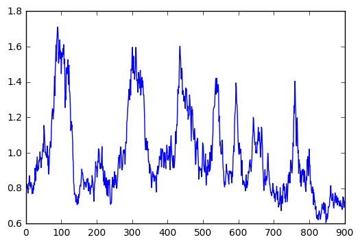
For simulations with zero change points we are interested in measuring statistical significance or confidence of the test statistic which can be understood as
In simulations with zero change points obviously is true. So, for a run of simulations we estimate confidence as
We run simulations without change points and vary certain fixed parameter while measuring confidence and inverse -value for each value of parameter. The only nontrivial results were obtained for change in data dimension .
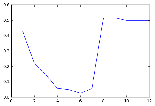
Additional experiments were conducted with growing variance and changes in covariance structure of the observations, however no dependencies were identified. This could be due to stabilizing effect of vector rank functions.
Simulations with One Change Point
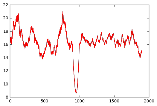
While running a simulations with one change point we are naturally interested in the estimation of statistical power of the test which can be understood as
and can be estimated for simulations as
We investigate dependence of on differences between distributions from opposite sides of the change point.
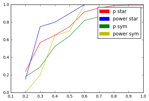
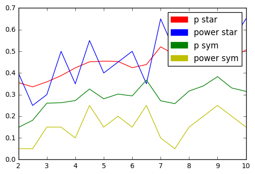
The figures shows that star discrepancy outperforms symmetric discrepancy in detecting change both in expectation and in variance. However empirical results in [18] indicates that in some situations symmetric discrepancy may turn out tob be a better tool.
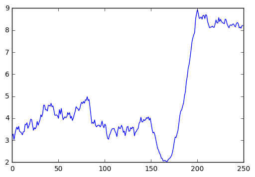
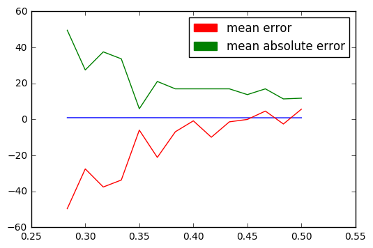
In the situation of existing change point not only power of the test is of interest but also a precision of change point estimations. As it was shown in previous chapter bias of a change point estimate increases as true ratio of distributions in the sample diverges from the value of . We provide a computational illustrations:
Simulations with Multiple Change Points
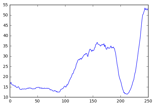
For case of multiple change point we provide only example with diphoragrams:
Examples with financial data:
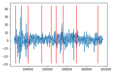
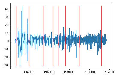
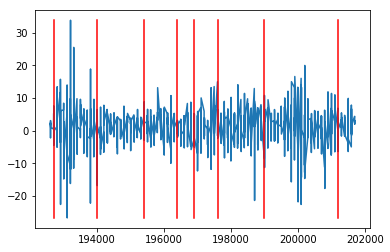
In order to provide examples, which are not artificially constructed, financial data similar to one in [31]. This data was acquired from Data library of Keneth R. French. It contains mean monthly returns from five portfolios each composed of one of five industrial sectors in the USA, which are:
-
(A)
Finance,
-
(B)
Manufacturing,
-
(C)
Retail, wholesale and some services,
-
(D)
Utilities,
-
(E)
Other.
This provides data dimension of and total number of observations of as they were recorded monthly from July of the year 1925 to the may of the year 2017.
(A) 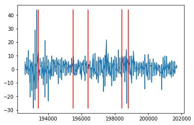 (B)
(B) 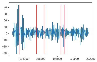 (C)
(C) 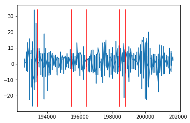
(D) 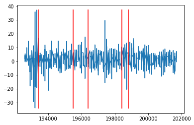 (E)
(E) 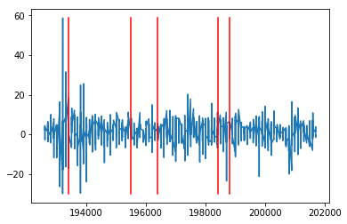
In the original paper [31] the parametric Bayesian inference was used too estimate nine and seven change points, and the total number of change point was only guessed and not inferred. Our results differ significantly from this original results, however different time range was used.
(A)
(B)
(C)
(D) 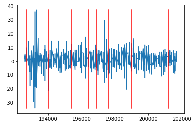 (E)
(E) 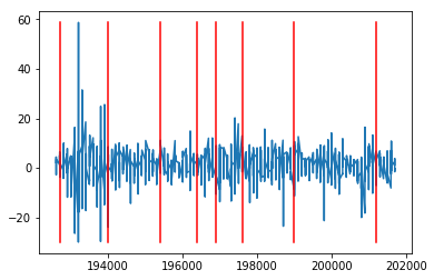
It can be projected that all above change points can be attributed to the important events in the economic history. For example, change point at July 1954 can be related to the end of recession of 1953, which itself can be explained by the change of interrelations of the industrial sectors leading to the change in the structure of the observed distribution. Hence, we can describe performance of the SMA-procedure as satisfactory.
Conclusion and Discussion
As result of the work a collection of methods of change point detection methods was developed. All this methods are based on interaction of vector ranks and geometric discrepancy which is a novel result. Certain basic consistency result were proved for the method in its basic form designed for detecting a single change point. However, they also can be applied for detecting and estimating multiple change points.
Computational results shows applicability of the method both for simple artificial change point problems an problems concerning actual data from applications. It is strictly indicated by resulting experience that the method is much more potent in situations then the distributions are not concentric. Empirical evidences of our theoretical findings were also observed. These theoretical results include expression of relation on different sides of change point through inner product in the Hilbert space . Another Theoretical result concerns dependence of estimate’s bias on ratio in which change point separates sample.
Another positive results is the discovery of , which can be used for establishing alternative iterative procedures defined by relations in this Hilbert space. Furthermore, this Hilbert space structure on empirical measures can be used for proving more theoretical results in the future.
Better proofs which cover ergodic processes and provide exact rates of convergence a still need to be worked out for the methods. Furthermore concentration results for change point estimates might render this algorithms interesting for practical application. However, they are absent in the current work.
Finally, online version of method can be implemented. The only requirement for this algorithm is fast online computation of the optimal assignment problem. It can be projected that such algorithm can be derived from the Sinkhorn distance regularised algorithm which were designed by Cuturi [7].
References
- [1] Ilya A Antonov and VM Saleev “An economic method of computing LP-sequences” In USSR Computational Mathematics and Mathematical Physics 19.1 Elsevier, 1979, pp. 252–256
- [2] Aleksandr Alekseevich Borovkov “Asymptotically optimal solutions in the change-point problem” In Theory of Probability & Its Applications 43.4 SIAM, 1999, pp. 539–561
- [3] E Brodsky and BS Darkhovsky “Nonparametric Methods in Change Point Problems” Springer Science & Business Media, 1993
- [4] Victor Chernozhukov, Alfred Galichon, Marc Hallin and Marc Henry “Monge-Kantorovich depth, quantiles, ranks, and signs”, 2014 arXiv:1412.8434 [stat.ST]
- [5] Christine Choirat and Raffaello Seri “The asymptotic distribution of quadratic discrepancies” In Monte Carlo and quasi-Monte Carlo methods 2004 Springer, 2006, pp. 61–76
- [6] Miklós CsörgHo and Lajos Horvath “20 Nonparametric methods for changepoint problems” In Handbook of statistics 7 Elsevier, 1988, pp. 403–425
- [7] Marco Cuturi “Sinkhorn distances: Lightspeed computation of optimal transport” In Advances in Neural Information Processing Systems, 2013, pp. 2292–2300 arXiv:1306.0895 [stat.ML]
- [8] Alexis Decurninge “Multivariate quantiles and multivariate L-moments”, 2014 arXiv:1409.6013 [math.ST]
- [9] A Dvoretzky, Jack Kiefer and Jacob Wolfowitz “Sequential decision problems for processes with continuous time parameter. Testing hypotheses” In The Annals of Mathematical Statistics 24.2 Institute of Mathematical Statistics, 1953, pp. 254–264
- [10] Meyer A Girshick and Herman Rubin “A Bayes approach to a quality control model” In The Annals of mathematical statistics JSTOR, 1952, pp. 114–125
- [11] Fred Hickernell “A generalized discrepancy and quadrature error bound” In Mathematics of Computation of the American Mathematical Society 67.221, 1998, pp. 299–322
- [12] Fred J Hickernell “Error Analysis for Quasi-Monte Carlo Methods”, 2017 arXiv:1702.01487 [math.NA]
- [13] Edmund Hlawka “Discrepancy and Riemann integration” In Studies in Pure Mathematics (New York) 3, 1971
- [14] L M Kantorovich “On the transfer of masses” In Dokl. Akad. Nauk. SSSR 37, 1942, pp. 227–229
- [15] Yoshinobu Kawahara and Masashi Sugiyama “Sequential change-point detection based on direct density-ratio estimation” In Statistical Analysis and Data Mining 5.2 Wiley Online Library, 2012, pp. 114–127
- [16] Albert Y Kim, Caren Marzban, Donald B Percival and Werner Stuetzle “Using labeled data to evaluate change detectors in a multivariate streaming environment” In Signal Processing 89.12 Elsevier, 2009, pp. 2529–2536
- [17] Harold W Kuhn “The Hungarian method for the assignment problem” In Naval research logistics quarterly 2.1-2 Wiley Online Library, 1955, pp. 83–97
- [18] Jia-Juan Liang, Kai-Tai Fang, Fred Hickernell and Runze Li “Testing multivariate uniformity and its applications” In Mathematics of Computation 70.233, 2001, pp. 337–355
- [19] Bruce G Lindsay “Mixture models: theory, geometry and applications” In NSF-CBMS regional conference series in probability and statistics, 1995, pp. i–163 JSTOR
- [20] Alexandre Lung-Yut-Fong, Céline Lévy-Leduc and Olivier Cappé “Homogeneity and change-point detection tests for multivariate data using rank statistics”, 2011 arXiv:1107.1971 [math.ST]
- [21] David S Matteson and Nicholas A James “A nonparametric approach for multiple change point analysis of multivariate data” In Journal of the American Statistical Association 109.505 Taylor & Francis, 2014, pp. 334–345 arXiv:1306.4933 [stat.ME]
- [22] Gaspard Monge “Mémoire sur la théorie des déblais et des remblais” In Histoire de l‘Académie Royale des Sciences de Paris, avec les Mémoires de Mathématique et de Physique pour la méme année De l’Imprimerie Royale, 1781, pp. 666–704
- [23] Vito MR Muggeo and Giada Adelfio “Efficient change point detection for genomic sequences of continuous measurements” In Bioinformatics 27.2 Oxford University Press, 2010, pp. 161–166
- [24] Harald Niederreiter “Quasi-Monte Carlo methods and pseudo-random numbers” In Bulletin of the American Mathematical Society 84.6, 1978, pp. 957–1041
- [25] Moshe Pollak “Optimal detection of a change in distribution” In The Annals of Statistics JSTOR, 1985, pp. 206–227
- [26] Filippo Santambrogio “Optimal transport for applied mathematicians” In Birkäuser, NY (due in September 2015) Springer, 2015
- [27] Robert Serfling “Quantile functions for multivariate analysis: approaches and applications” In Statistica Neerlandica 56.2 Wiley Online Library, 2002, pp. 214–232
- [28] WA Shewhart “The application of statistics as an aid in maintaining quality of a manufactured product” In Journal of the American Statistical Association 20.152 Taylor & Francis Group, 1925, pp. 546–548
- [29] Albert N Shiryaev “On optimum methods in quickest detection problems” In Theory of Probability & Its Applications 8.1 SIAM, 1963, pp. 22–46
- [30] I Sobol and Yu L Levitan “The production of points uniformly distributed in a multidimensional cube” In Preprint IPM Akad. Nauk SSSR 40.3, 1976
- [31] Makram Talih and Nicolas Hengartner “Structural learning with time-varying components: tracking the cross-section of financial time series” In Journal of the Royal Statistical Society: Series B (Statistical Methodology) 67.3 Wiley Online Library, 2005, pp. 321–341
- [32] N Tomizawa “On some techniques useful for solution of transportation network problems” In Networks 1.2 Wiley Online Library, 1971, pp. 173–194
- [33] Cédric Villani “Optimal transport: old and new” Springer Science & Business Media, 2008
- [34] Hermann Weyl “Über die gleichverteilung von zahlen mod. eins” In Mathematische Annalen 77.3 Springer, 1916, pp. 313–352